CLIMATIC EFFECTS ON THE PHENOLOGY OF GEOPHYTES
B.EPPICH1–L.DEDE 1–A.FERENCZY1–Á.GARAMVÖLGYI1–L.HORVÁTH2–I.ISÉPY3– SZ.PRISZTER3–L.HUFNAGEL2*
1Department of Mathematics and Informatics, Corvinus University of Budapest, Faculty of Horticulture, H-1118 Budapest, Villányi út 29-43., Hungary
(phone: +36-1-482-6261; fax: +36-1-466-9273)
2“Adaptation to Climate Change” Research Group, Hungarian Academy of Sciences, Office for Subsidised Research Units, H-1118 Budapest, Villányi út 29-43., Hungary
(phone: +36-1-482-6261; fax: +36-1-466-9273)
3Botanical Garden, Eötvös Loránd University, Faculty of Science H-1083 Budapest, Illés utca 25., Hungary
*Corresponding author e-mail: leventehufnagel@gmail.com
(Received 28th August 2009 ; accepted 24th November 2009)
Abstract. Nowadays, the scientific and social significance of the research of climatic effects has become outstanding. In order to be able to predict the ecological effects of the global climate change, it is necessary to study monitoring databases of the past and explore connections. For the case study mentioned in the title, historical weather data series from the Hungarian Meteorological Service and Szaniszló Priszter’s monitoring data on the phenology of geophytes have been used. These data describe on which days the observed geophytes budded, were blooming and withered. In our research we have found that the classification of the observed years according to phenological events and the classification of those according to the frequency distribution of meteorological parameters show similar patterns, and the one variable group is suitable for explaining the pattern shown by the other one. Furthermore, our important result is that the dates of all three observed phenophases correlate significantly with the average of the daily temperature fluctuation in the given period. The second most often significant parameter is the number of frosty days, this also seem to be determinant for all phenophases. Usual approaches based on the temperature sum and the average temperature don’t seem to be really important in this respect.
According to the results of the research, it has turned out that the phenology of geophytes can be well modelled with the linear combination of suitable meteorological parameters
Keywords: climate change, phenophases, meteorology, cluster analysis, correlation, phenological models.
Introduction
Climate change is one of the most important ecological problems of our times [13]. It is of great significance because it affects the living conditions of the whole global society [10]. Challenges and tasks related to the climate change determine almost all segments of the society and economy fundamentally [4]. Climate policy includes among others several issues of the agriculture and food production, land use, energetics, industry and transport, environmental and nature conservation and public health, but it also has sociological, educational, communication, even safety policy and foreign policy aspects. Changeability of the climate that is the lack of climatic stability in longer periods (and its degree) is determinant for the state and change of state of all earthly ecosystems [7, 8, 11, 16, 17, 20, 29]. The degree of the changeability of the climate (the total variability of the climatic parameters) shows in itself significant heterogeneity both
in space (regionally) and time (according to time slots of research). The degree of the changeability and its pattern in space and time are considerably scale dependant attributes at the same time. A further methodological problem is implied by the fact that not only the active component (the changeability of the climate in this case) but also the different, natural and human-influenced ecosystems (as the systems receiving the effects) show fundamental heterogeneity from the point of view of their sensitivity to the effect [12, 26, 27]. Sensitivity can be characterized by the change of state and its dynamics caused by unit effect in this context. Moreover, ecosystems as systems capable of regulation do not endure effects passive but they react to those with adaptation and feedback of different degree and type [6]. In the case of human- influenced ecosystems, this adaptation would require optimising human activity and intervention, which still has significant methodological faultiness nowadays. All these circumstances, the climatic effect and the reactions of the ecosystems as well as human activity play a determinand role in the sustainability of ecosystems and its risks. Among basic ecological phenomena, climate change influences seasonal community dynamics and one of its important factors, the phenology of the species, most strongly [24, 30].
Therefore, in our present study the connection between weather conditions and phenology was examined using Szaniszló Priszter’s phenological monitoring data series on geophytes.
In our research we have set three main goals:
1. To explore according to some suitably chosen years whether frequency distributions of the meteorological parameters in the given period play a determinant role in the development of phenological patterns.
2. To survey with the help of correlational analyses, which meteorological parameters have what kind of influence on the phenological behaviour of the individual indicator plants.
3. To examine whether new variables made by linear combinations of meteorological parameters can lead to working out effective phenological models, which could play a role in future climate change research.
Review of Literature
Phenological data collected by research systems all over the world aid with making models and with the help of their statistical analysis the degree of the global warming can be predicted.
In China, it is the CAS network that examines different phenophases [2]. There are both woody and herbaceous plants among the 173 species examined and different phenophases of these plants such as budding or autumn colouring are observed. These data are used to examine their correlation with meteorological parameters. The CAM network collects different meteorological data on 587 stations. Models show to what extent the date of the blooming of the individual plants differs in various regions of China, which is brought into connection with temperature and carbon dioxide concentration.
Japan’s network called JMA was founded in 1953 [2]. It has nearly 100 stations, which observe phenophases and collect meteorological data. Phenological models concentrate mainly on the normal phenophase, the effect of the warming of urban regions and the climate change. One of these models shows the relationship between the
main blooming and geographical coordinates, while another relationship between temperature and blooming.
In Australia, mainly Eucalyptus species are observed [15] but Araucaria cumminghamii, Corymbia maculata and Pinus species are also examined.
The first phenological network in Europe is linked with the name of Carl von Linné, who made his observations in Sweden [18]. The International Phenological Garden (IPG) is nowadays a unique system in Europe, which was founded by F. Schnelle and E.
Volkert in 1957. It observes 7 phenophases of 23 plant species and measures the growing period, the concentration of carbon dioxide and the change of spring temperature. There are networks in several countries of Europe, such as in Albania, Austria, the Czech Republic, Estonia, Germany, Poland, Russia, Slovakia, Slovenia, Spain and Switzerland. There are incomplete systems for example in Portugal and Greece.
Research in the USA mainly began in the 20th century [24]. Between 1851-1859 86 plant species and insects were observed in 33 places. In the 1950s, research of the phenology became important for the agriculture. Beside Syringa and Lonicera species, the observation of Cercis canadensis, Cornus florida and Acer rubrum is significant.
In Canada, first nations and Inuits made a natural calendar, which showed the date of blooming of Thermopsis rhombifolia, the rosaceae and Holodiscus discolor as well as the ripening of Rubus spectabilis [24]. Nowadays blooming of wild flowers, phenology of birds and frogs and freezing of lakes and rivers are observed.
In South-America, blooming of indigenous tropical trees such as coffee and cacao are observed [19]. Research is carried out related to climate change, El Niño and the effects of carbon dioxide emission on plant phenology.
Researchers started to show interest in phenological observations mainly in the 1990s [1]. They have mostly been motivated by the recently risen temperature and changes in the development of plants and animals. The Phenology Study Group was established in Canada in 1993, then the Global Phenological Monitoring (GPM) in 1996. GPM is an important system in the northern hemisphere. A phenophase mostly depends on the temperature, precipitation, soil type, soil humidity and the sunshine. The most significant from these is the effect of the temperature therefore GPM focuses on it.
Criteria of the selection of the species for observation:
Plants should have phenophases that are easy to observe.
The start of the phenophases should be sensitive to air temperature.
Plants should be economically important.
Plants should have a broad geographic distribution or ecological amplitude.
Plants should be easy to propagate.
Blooming should last several months during the growing period.
These criteria are met particularly by fruit trees, bushes in parks and spring flowers.
There are special standardized observation programmes when plants are grown in a closed place, watered and eliminating weather effects. In these cases, only temperature effects are examined.
One of the most important phenological models is the plant development model. It goes back to 1735 and is linked with the name of Réaumur [3]. He recorded the dates of phenophases and the mean temperature measured on any day of the phenophase.
Modelling began to develop in the 20th century when computer sciences and examinations related to global climate change were also developing. It was mainly based on the relationship between the rise in temperature and the change of the
phenophases. Most models predict the date of budding, blooming and ripening, however, they cannot really prognosticate autumn colouring of the trees yet.
Models have three main types:
Theoretical: it is based on the cost-benefit ratio in the case of leaves put forth by the plants.
Statistical: it examines the relationship between climate factors and dates of the phenophases.
Mechanical: it describes known or assumed cause-and-effect dependences between biological processes and some environmental factors. For example, the spring warming model contains beside mean temperature and heat summation development rates as well. However, this model has a fundamental problem: our knowledge related to biochemical and biophysical processes in dormancy is rather insufficient.
Materials and Methods
We have used historical weather data series from the Hungarian Meteorological Service and Szaniszló Priszter’s observations of the phenology of geophytes for the case study. Szaniszló Priszter, the former director of the Botanical Garden of the Eötvös Loránd University has been observing and recording dates of occurrence of three characteristical phenophases of about 200 plant species, mainly geophytes for approximately 40 years in the last decades of the twentieth century [14, 21, 22, 23].
Priszter’s data have been substituted for day serial numbers in the individual years.
These data describe on which days the observed geophytes budded, were blooming and withered. Our database has been constructed from this mass of data and it contains Latin names of the species and day serial numbers of the occurrence of the three phenological events for each examined year. The Hungarian Meteorological Service has published hundred-year daily data of Budapest for a long time, among which you can find the daily mean temperature, the daily maximum and minimum temperature, tha amount and type of daily precipitation and the daily sunshine duration. In order to complete these, radiation values have also been calculated (according to [28]).
Examining the connection between phenological parameters and weather, we have used three approaches:
From the meteorological data series, the yearly frequency distribution of the characteristical meteorological parameters has been calculated for the ecologically effective period of each year, then the years have been classified according to these data. The same years have been classified according to the phenological indicators (day serial numbers of the occurrence of phenophases of a given species) as well, then classifications made for the same objects (years) but according to different variables have been compared.
As a second approach, correlation between the individual phenological indicators and weather parameters has been examined separately. For this purpose, a meteorological parameter vector containing 24 elements has been made for the period in which the phenological change of state of the given plant in the current year has been examined (from 28th August in the previous year and from 27th August in leap year respectively, till the current phenological change). In order that the result of the research is utilizable for further climate change research, daily global radaiation values have also been determined
according to the Szász Gábor algorithm [28]. This method calculates daily global radiation values (W/m2) from the daily sunshine duration. The following derived meteorological parameters have been calculated:
1. average of daily global radiation (met1), 2. average of daily mean temperature (met2), 3. average of daily maximum temperature (met3), 4. average of daily minimum temperature (met4), 5. precipitation amount (met5),
6. sunshine duration (met6),
7. daily average of sunshine duration (met7), 8. number of days with precipitation (met8),
9. number of days with real precipitation (excluding trace of precipitation) (met9),
10. sum of mean temperature > 10 °C (met10), 11. sum of mean temperature > 9 °C (met11), 12. sum of mean temperature > 8 °C (met12), 13. sum of mean temperature > 7 °C (met13), 14. sum of mean temperature > 6 °C (met14), 15. sum of mean temperature > 5 °C (met15), 16. sum of mean temperature > 4 °C (met16), 17. sum of mean temperature > 3 °C (met17), 18. sum of mean temperature > 2 °C (met18), 19. sum of mean temperature > 1 °C (met19), 20. sum of mean temperature > 0 °C (met20),
21. average of daily temperature fluctuation (maximum-minimum) (met21), 22. relative deviation of precipitation for days with precipitation (met22), 23. number of frost days (met23),
24. sum of nonnegative daily mean temperature after the last frost day till the day of the phenological change (met24).
Using these meteorological indicators, analyses of correlation have been carried out of the phenophases in our geophytes’ phenology database for each year of examination.
For our work the statistical software package PAST [9] has also been used [5]. We have tried to make an index (G index) so that values on the left side meaning full acceptance have been counted with double weight and values on the right side meaning almost- acceptance have been counted once, and the sum of these has been divided by sixfold of the number of the evaluated plants (93) since three phenological changes of each plant species has been considered (Table 1).
As a third approach, linear combinations have been made of the individual meteorological indicators, then, optimizing their parameters with the help of the Solver adds-on of MS Excel, explanatory models for the phenological indicators have been searched for.
Results
Classification of years according to phenological and meteorological characteristics In our research, first we wanted to know whether there is a similar aggregation or an outstanding, specific year between general characteristics such as frequency distribution of different meteorological parameters and the date of phenological phenomena in the years 1978–1997. We have used hierarchical cluster analysis with Euclidean and simple average method. Classification according to phenological parameters can be seen in Figure 1 and classification according to meteorological indicators in Figure 2.
0 1.6 3.2 4.8 6.4 8 9.6 11.2 12.8 14.4 16
-200 -180 -160 -140 -120 -100 -80 -60 -40 -20
Similarity 96 94 92 95 97 79 78 81 91 83 84 93 80 82 85
Figure 1. Classification of the years of examination according to the phenological behaviour of some indicator species. It can be seen that the year 1996 definitely separates from the other
years. The years 1982, 1985 and 1994 also have different behaviour than the majority.
0 1.6 3.2 4.8 6.4 8 9.6 11.2 12.8 14.4 16
-90 -80 -70 -60 -50 -40 -30 -20 -10
Similarity 96 85 91 79 97 78 81 84 82 93 92 83 95 80 94
Figure 2. Classification of the years of examination according to the frequency distribution of meteorological parameters. The year 1996 definitely separates from the others according to this
classification, too.
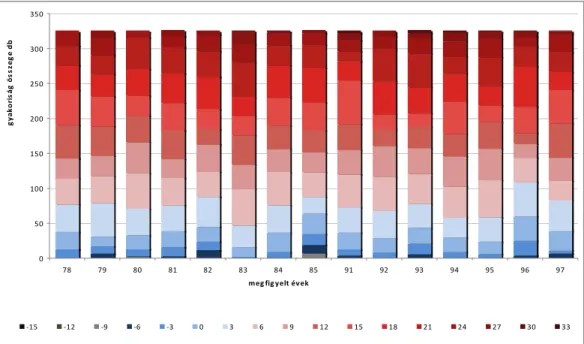
A frequency table has been made of the most important meteorological parameters for the years of examination (from 28th August of the previous year to 20th July of the current year), the diagrams of which can be seen below (Figures 3-7).
Figure 3. Distribution of the daily minimum temperature in the years of examination. The number of days with low minimum temperature was definitely higher in 1996 than in other
years. The greater proportion of cold days is also characteristic for 1982 and 1985.
0 50 100 150 200 250 300 350
78 79 80 81 82 83 84 85 91 92 93 94 95 96 97
meg fig yelt évek
gyakoriság összege db
-15 -12 -9 -6 -3 0 3 6 9 12 15 18 21 24 27 30 33
Figure 4. Frequency of daily average temperature. The number of days with lower average temperature was slightly bigger in 1996 than in other years
0 50 100 150 200 250 300 350
78 79 80 81 82 83 84 85 91 92 93 94 95 96 97
megfiegyelt évek
gyakoriságok összege db
-14 -11 -8 -5 -2 1 4 7 10 13 16 19 22 25
0 50 100 150 200 250 300 350
78 79 80 81 82 83 84 85 91 92 93 94 95 96 97
vizsgált évek
ingadozás-gyakoriságok összege db
1.5 3.0 4.5 6.0 7.5 9.0 10.5 12.0 13.5 15.0 16.5 18.0 19.5
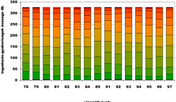
Figure 5.Distribution of the daily temperature fluctuation in the years of examination. 1996 can be considered as typical from this point of view. 1985 excels in the high frequency of days
with lower temperature fluctuation.
30 55 80 105 130 155 180 205 230 255 280 305 330
78 79 80 81 82 83 84 85 91 92 93 94 95 96 97
vizsgált évek
gyakoriságok összege
0 1 2 3 4 5 6 7 8 9 10 11 12 13 14 15
Figure 6. Distribution of the sunshine duration in the years of examination. 1996 can be considered as ordinary from this point of view, too.
130 150 170 190 210 230 250 270 290 310 330
78 79 80 81 82 83 84 85 91 92 93 94 95 96 97 megfigyelt évek
megfigyelt évek megfigyelt évek megfigyelt évek gyakoriságok összege dbgyakoriságok összege dbgyakoriságok összege dbgyakoriságok összege db
0 0.0001 3 6 9 12 15
18 21 24 30 40 50 60
70 80 90 100 150 200 300
Figure 7. Trend of the frequency of precipitation in the periods of examination. 1996 is ordinary from this point of view, too. The proportion of days with much precipitation is the
biggest in 1994.
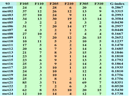
Correlation between phenological indicators and derived meteorological parameters In the table, rows represent calculated meteorological attributes and cells mean the number of events of the correlation between the three phenophases’ date of occurrence and the given meteorological indicator accepted at 95% and 90% significance level as well as the values of G index calculated from these.
Table 1.Correlation evaluation table. Cells contain the number of events of the correlation between calculated meteorological paramteres (rows) and the three phenophases’ date of occurrence (columns) accepted at 95% and 90% significance level as well as vales of G index. The average of daily temperature fluctuation for the given period (met21) has most often correlated significantly with the date of all three phenophases. The second most often significant parameter is the number of frost dyas (met23).
93 F105 F110 F205 F210 F305 F310 G-index
met01 24 4 28 6 20 6 0.2867
met02 37 12 26 12 13 9 0.3315
met03 37 10 24 9 11 4 0.2993
met04 34 13 30 19 13 14 0.3584
met05 3 2 2 4 3 2 0.0430
met06 31 7 20 14 17 8 0.2957
met07 4 3 2 1 3 3 0.0448
met08 27 10 5 7 4 4 0.1667
met09 11 7 20 12 26 15 0.2652
met10 10 11 5 3 10 5 0.1237
met11 17 5 6 2 14 1 0.1470
met12 20 6 7 3 14 3 0.1685
met13 21 7 8 3 15 5 0.1846
met14 23 5 9 1 14 3 0.1810
met15 23 6 9 1 13 3 0.1792
met16 25 3 9 2 14 3 0.1864
met17 25 3 10 1 15 4 0.1935
met18 24 3 10 1 12 5 0.1810
met19 24 3 10 11 5 0.1756
met20 25 3 8 2 11 5 0.1756
met21 85 3 71 6 69 7 0.8351
met22 2 7 2 6 3 2 0.0520
met23 62 8 53 10 20 15 0.5430
met24 12 10 14 4 12 7 0.1738
Modelling phenological phenomena using linear combinations of meteorological parameters
In the future, strong statistical models will be needed for the comparative evaluation of climate change scenarios, which are able to characterize the behaviour of indicated variables according to indicating variables.
As a first step of making these models, linear combinations have been made of the individual meteorological indicators, then optimizing their parameters with the help of Solver adds-on of MS Excel, well-fitting models have been searched for, which can be used later as starting hypotheses to develop more complex and reliable models. Now some promising results of our initial attempts are presented (Figure 8).
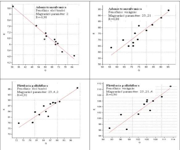
Figure 8. Correlation between linear combinations calculated from some meteorological parameters and the date of occurrence of the modelled phenophase using the example of two
phenophases (first bud and blooming) of two species (Adonis transsilvanica and Fritillaria pallidiflora).Appearance of the first bud of Adonis transsilvanica can be explained by only one
meteorological variable, the average of daily mean temperature. However, the beginning of blooming can be well explained by the linear combination made of the number of frost days and
the average of daily temperature fluctuation. The phenological behaviour of Fritillaria pallidiflora can be explained by the linear combination of three meteorological variables (number of frost days, average of daily minimum temperature as well as average of daily mean
temperature and temperature fluctuation, respectively)
Discussion
Classification of years according to phenological and meteorological characteristics According to classifications on the basis of both phenological parameters and meteorological indicators, it is striking that 1996 definitely separates from the other years (Figure 1 and 2). Its explanation becomes clear if the frequency distribution of daily minimum temperature is examined (Figure 3). It can be observed that the number of days with lower minimum temperature was definitely higher in 1996 than in other years (just as the number of days with lower mean temperature, but not so striking) (Figure 4). As for precipitation amount, daily temperature fluctuation and sunshine duration, 1996 can be rather considered as ordinary, however (Figure 5, 6 and 7).
As for phenological behaviour, the years 1982, 1985 as well as 1994 have differnet behaviour than the majority of years. Greater proportion of cold days is characteristic for both 1982 and 1985 but 1985 excels in the frequency of days with smaller temperature fluctuation as well. However, the separation of 1994 is caused by an other factor: the proportion of days with much precipitation is the biggest then (Figure 7).
Correlation between phenological indicators and derived meteorological parameters Examining 93 geophytes, it can be stated that the average of daily temperature fluctuation for the given period (the difference between daily maximum and minimum temperature, met21) has most often correlated significantly with the date of all three phenophases (Table 1). It is surprising because models used in phenology usually yield good results using parameters related to heat summation or mean temperature. The second most often significant parameter is the number of frost days (met23), it also seems to be determinant regarding all three phenophases and this is not surprising because these are spring flowers, which can be obviously limited by frost.
However, the other factors differ per phenophase. The appearance of the first buds can be affected by the average of daily maximum temperature (met3) and the average of daily mean temperature (met2) apart from the above, which is easy to understand because this is in connection with spring warming, obviously.
However, the blooming date is rather affected by the average of daily minimum temperature (met4) and global radiation (met1), which can be caused by the fact that the blooming of the developed buds can be limited by low temperature at night or early morning.
The date of withering is often influenced by a factor that almost never affects the previous two phenophases, this is the number of days with real precipitation (met9), which seems to be even more important than the number of frost days (met23) in this case. This is also clear because it is not the thermal but the precipitation conditions which dominate when withering.
It is also extremely interesting to examine which meteorological parameters almost never (that means very rarely) affect the phenology of geophytes. These are the precipitation amount (met5) and the relative deviation of precipitation for days with precipitation (met22). Ineffectiveness of the variables describing precipitation conditions is not surprising because geophytes are able to tolerate lack of precipitation due to their storage organs so they are not exposed to precipitation conditions as much.
However, the daily average of sunshine duration (met7) and the sum of mean temperature above 10 °C (met10) do not seem to be effective either, which is surprising
because sunshine and heat usually are important factors in case of phenological phenomena.
Our results point out that the phenology of geophytes mostly depends on the fluctuation of temperature and limiting factors.
Modelling phenological phenomena using linear combinations of meteorological parameters
It can be seen in the figures (Figure 8) that the appearance of the first bud of Adonis transsilvanica can be well explained by only one meteorological variable (that means without using linear combinations), this variable is the average of daily mean temperature, which does not belong to the most significant variables in the case of most of our plants but it has an important role in the case of this species. However, the beginning of blooming can be explained not by this parameter but the linear combination made of the number of frost days and the average of daily temperature fluctuation.
The phenological behaviour of Fritillaria pallidiflora can only be explained by the linear combination of three-three meteorological variables. The number of frost days and the average of daily minimum temperature play a role in both phenophases (appearance of the first bud and blooming) but in the case of the first bud the average of daily mean temperature, in the case of blooming the fluctuation of temperature has to be added moreover.
These results show the usefulness of the method used but also the fact that different factors have an important effect on different phenophases of various plants.
Outlook
The results presented in this paper methodologically enable the comparative evaluation and analysis of the GCM outputs based on climate change scenarios and especially those of their dynamically or statistically downscaled data series related to future climate. Considering this, it seems to be advisable in the future to examine phenological effects of climate change with the help of strategic system models and tactical models based on data, too. Significant progress can be reached by combining statistical and simulation methodology and using theoretical modelling, empirical data collection and monitoring together.
Acknowledgements. Our research has been supported by the research proposal OTKA TS 049875 (Hungarian Scientific Research Fund); the VAHAVA project; the KLIMA-KKT project (National Office for Research and Technology, Ányos Jedlik Programme); the Adaptation to Climate Change Research Group (Hungarian Academy of Sciences, Office for Subsidised Research Units); the Research Assistant Fellowship Support (Corvinus University of Budapest) and the “Bolyai János” Research Fellowship (Hungarian Academy of Sciences, Council of Doctors). We thank Nándor Fodor algorithm developer for his work, which has enabled us to use the Szász Gábor-algorithm of global radiation in MS Excel.
REFERENCES
[1] Bruns, E., Chmielewski, F.-M., van Vliet, A.J.H. (2003): The Global Phenological Monitoring Concept. – In: Schwartz, M.D. (ed.) Phenology: An Integrative Environmental Science, Kluwer Academic Publishers, The Netherlands.
[2] Chen, X. (2003): East Asia. – In: Schwartz, M.D. (ed.) Phenology: An Integrative Environmental Science, Kluwer Academic Publishers, The Netherlands.
[3] Chuine, I., Kramer, K., Hänninen, H. (2003): Plant Development Models. – In: Schwartz, M.D. (ed.) Phenology: An Integrative Environmental Science, Kluwer Academic Publishers, The Netherlands.
[4] Csete, M., Török, Á. (2008): Települések klímavédelemmel összehangolt fejlesztési beruházásainak optimalizálása. – Klíma-21 54: 91-97.
[5] Dede, L., Eppich, B., Ferenczy, A., Horváth, L., Hufnagel, L., Isépy, I. (2009): Történeti időjárási adatbázis alkalmazási lehetőségei. – Agrárinformatika 209, Debrecen, 2009.
augusztus 26-27. (in press)
[6] Drégelyi-Kiss, Á., Drégelyi-Kiss, G., Hufnagel, L. (2008): Ecosystems as climate controllers – biotic feedbacks (a review). – Applied Ecology and Environmental Research 6(2): 111-135.
[7] Erdélyi, É. (2008): Az őszi búza termeszthetőségi feltételei az éghajlatváltozás függvényében. Doktori (PhD) értekezés. – Budapesti Corvinus Egyetem, Kertészettudományi Kar, Matematika és Informatika Tanszék, Budapest.
[8] Gaál, M. (2008): Expected changes in climatic conditions of main crops. – Klíma-21. 55:
28-35.
[9] Hammer, Ř., Harper, D.A.T., Ryan, P.D. (2001): PAST: Paleontological Statistics Software Package for Education and Data Analysis. – Palaeontologia Electronica 4(1): 9.
http://palaeo-electronica.org/2001_1/past/issue1_01.htm
[10] Harnos, Zs., Gaál, M., Hufnagel, L. (szerk.) (2008): Klímaváltozásról mindenkinek. – Budapesti Corvinus Egyetem, Budapest.
[11] Hufnagel, L., Gaál, M. (2005): Seasonal dynamic pattern analysis in service of climate change research. – Applied Ecology and Environmental Research 3(1): 79-132.
[12] Hufnagel, L., Sipkay, Cs., Drégelyi-Kiss, Á., Farkas, E., Türei, D., Gergócs, V., Petrányi, G., Baksa, A., Gimesi, L., Eppich, B., Dede, L., Horváth, L. (2008): Klímaváltozás, biodiverzitás és közösségökológiai folyamatok kölcsönhatásai. – In: Harnos, Zs., Csete, L. (szerk.) Klímaváltozás: Környezet - Kockázat - Társadalom, Szaktudás Kiadó Ház, Budapest.
[13] IPCC (2007): Climate Change 2007: Synthesis Report. Contribution of Working Group I, II and III to the Fourth Assessment Report of the Intergovernmental Panel of Climate Change. – IPCC, Geneva, Switzerland.
[14] Isépy, I., Priszter, Sz. (1972): Chorologische und phänologische Untersuchungen an mediterranen Geophyten. I. Narcissus. – Annal. Univ. Sci. Budapest, Sect. Biol. 14.: 105- 117.
[15] Keatley, M.R., Fletcher, T.D. (2003): Australia. – In: Schwartz, M.D. (ed.) Phenology:
An Integrative Environmental Science, Kluwer Academic Publishers, The Netherlands.
[16] Ladányi, M. (2008): Viticulture challenges under changing climate in Hungary. – Klíma- 21. 55: 36-52.
[17] Ladányi, M., Hufnagel, L. (2006): The effect of climate change on the population of sycamore lace bug (Corythuca ciliata, SAY, Tingidae Heteroptera) based on a simulation model with phenological response. – Applied Ecology and Environmental Research 4(2):
85-112.
[18] Menzel, A. (2003): Europe. – In: Schwartz, M.D. (ed.) Phenology: An Integrative Environmental Science, Kluwer Academic Publishers, The Netherlands.
[19] Morellato, L.P.C. (2003): South America. – In: Schwartz, M.D. (ed.) Phenology: An Integrative Environmental Science, Kluwer Academic Publishers, The Netherlands.
[20] Őszi, B., Ladányi, M., Hufnagel, L. (2006): Population dynamics of the Sycamore Lace Bug, Corythuca ciliata (Say) (Heteroptera: Tingidae) in Hungary. – Applied Ecology and Environmental Research 4(1): 135-150.
[21] Priszter, Sz., Isépy, I. (1974): Chorologische und phänologische Untersuchungen an mediterranen Geophyten. II. Galanthus. – Annal. Univ. Sci. Budapest, Sect. Biol. 16.: 87- 101.
[22] Priszter, Sz. (1960-2000): Fenológiai adatbázis (kézirat). – ELTE TTK Botanikus kert könyvtára, Budapest.
[23] Priszter, Sz. (1974): Hagymás kerti virágok. – Mezőgazdasági Kiadó, Budapest, 219.
[24] Schwartz, M.D. (ed.) (2003): Phenology: An Integrative Environmental Science. – Kluwer Academic Publishers, Dordrecht/Boston/London.
[25] Schwartz, M.D., Beaubien, E.G. (2003): North America. – In: Schwartz, M.D. (ed.) Phenology: An Integrative Environmental Science, Kluwer Academic Publishers, The Netherlands.
[26] Sipkay, Cs., Horváth, L., Nosek, J., Oertel, N., Vadadi-Fülöp, Cs., Farkas, E., Drégelyi- Kiss, Á., Hufnagel, L. (2008): Analysis of climate change scenarios based on modelling of the seasonal dynamics of a Danubian copepod species. – Applied Ecology and Environmental Research 6(4): 101-108.
[27] Sipkay, Cs., Hufnagel, L., Révész, A., Petrányi, G. (2007): Seasonal dynamics of an aquatic macroinvertebrate assembly (Hydrobiological case study of Lake Balaton No. 2).
– Applied Ecology and Environmental Research 5(2): 63-78.
[28] Szász, G. (1968): A globálsugárzás összegeinek meghatározása számítás útján. – Debreceni Agrártudományi Főiskola Tudományos Közleményei XIV.: 239-253.
[29] Szenteleki, K., Ladányi, M., Szabó, É., Horváth, L., Hufnagel, L., Révész, A. (2007): A climate research database management software EFITA/WCCA, 2-5 July 2007, Glasgow, Scotland – Paper CD ROM p. 53.
[30] Vadadi-Fülöp, Cs., Hufnagel, L., Sipkay, Cs., Verasztó, Cs. (2008): Evaluation of climate change scenarios based on aquatic food web modelling. – Applied Ecology and Environmental Research 6(1): 1-28.
Electronic information source
Hungarian Meteorological Service: daily meteorological data of Budapest in the 20th century on the home page of the Hungarian Meteorological Service
http://met.hu/pages/climate/bp/Navig/Index2.htm