Effects of Temperature – Climate Patterns on the Production of Some Competitive Species on Grounds of Modelling
Ágota Drégelyi-Kiss&Levente Hufnagel
Received: 29 January 2009 / Accepted: 10 December 2009
#Springer Science+Business Media B.V. 2010
Abstract Climate change has serious effects on the setting up and the operation of natural ecosystems. Small increase in temperature could cause rise in the amount of some species or potential disappearance of others. During our researches, the dispersion of the species and biomass production of a theoretical ecosystem were examined on the effect of the temperature–climate change. The answers of the ecosystems which are given to the climate change could be described by means of global climate modelling and dynamic vegetation models. The examination of the operation of the ecosystems is only possible in huge centres on supercomputers because of the number and the complexity of the calculation. The number of the calcula- tion could be decreased to the level of a PC by considering the temperature and the reproduction during modelling a theoretical ecosystem, and several important theoretical questions could be answered.
Keywords Climate modelling . Ecosystem . Biomass production
1 Introduction and Aims
Direct and indirect effects of the climate change on the terrestrial and oceanic ecosystems could also be observed in the last decades. Researches show that there are changes in
phenological, morphological and physiological properties of taxa and changes in spread of species, in frequency of epidemics. But the potential effects of climate change on natural ecosystems and the answers given by living communities are less known. This is because of the complexity of natural ecosystems.
There are changes in the spread and local abundance of wild regional species which are caused by climate warming during the last years. Parmesan et al. [13] have studied 57 European butterflies in order to separate the climatic and non-climatic effects on the spread of the animals. There was a systematic shift northwards in the spread of most of the studied species during the twentieth century. There were data on 35 species related to the northern and southern borders of their spread; the area of two thirds of these species has shifted northwards by 30–240 km, and 6% of them has shifted southwards.
There are similar results in local researches related to some plants in the Alps in Switzerland and birds in Costa Rica.
Similarly, the red fox has gone northwards to the territory of the arctic fox, while the arctic fox has gone back to the poles [5]. Summarising the results of the researches, climate change has an important effect on natural populations.
Several scientists have examined theEuphydrias edithafor 40 years. It seems that the dynamic of the local population is managed by extreme weather conditions; therefore, the borders of its expansion are affected by the climate [13].
The important community–ecological researches have three main approaches related to methodology considering climate change. Ecologists working in the field observing real natural processes have aspired to interfere as little as possible with the processes [21]. The aim is to describe the community ecological patterns unbiased [9–11].
The other school of ecological researches examines hypotheses about natural processes. The basis of these researches is testing different predictions in manipulative trials [17]. The third part of ecologists deals with modelling Á. Drégelyi-Kiss (*)
Bánki Donát Faculty of Mechanical Engineering, Budapest Tech, 1081 Budapest Népszínház u. 8.,
Hungary
e-mail: dregelyi.agota@bgk.bmf.hu L. Hufnagel
Department of Mathematics and Informatics, Corvinus University of Budapest,
1118 Budapest Villányi út 29-43, Hungary
DOI 10.1007/s10666-009-9216-4
where a precise mathematical model is made for basic and simple rules of the examined phenomena.
The work of the modelling ecologists consists of two parts.
The first one is testing the mathematical model with case studies, and the second one is developing (repairing and fitting again) the model. These available models are sometimes far away from the observations of field ecologists because there are different viewpoints. In the course of modelling, the purpose is to simplify the phenomena of nature; in case of field observations, ecosystems appear as complex phenomena.
It is obvious that all the three approximations have advantages and disadvantages. There are two approaches:
monitoring- and hypothetic-centred approximations. In the course of monitoring approaches, the main purpose is to discover the relationships and patterns among empirical data. This is a multidimensional problem where the tools of biomathematics and statistics are necessary. Data originate from large monitoring systems (e.g. national light trap network, long-term ecological research).
In case of hypothetic-centred approaches, known or assumed relationships mean the starting point. There are three types of researches in this case:
& Testing simple hypotheses with laboratory or field
experiments (e.g. fitotron plant growing room)
& Analysing given ecosystems with tactical models (e.g.
local case studies, vegetation models, food web models, models of biogeochemical cycles) [5,6,19,22]
& Examination of general questions with strategic model-
ling (e.g. competition and prediction models, cell- automats, evolutionary–ecological models)
Our aim is to analyse the effect of some temperature–
climate patterns on the production and community–ecological relations in a strongly simplified theoretical model. The novelty of this modelling is characterised by a guild-specific approach at first (where competitive relationships can be manifested); on the other hand, the population-dynamic model has been connected with the outputs of global circulation models. So, this connection enables us to examine directly the effects of climate change.
2 Material and Methods
During our examinations, the behaviour of a theoretical ecosystem is studied by variously changing the temperature.
The simulation was made by Excel with simple mathematical background. An algae community in a terrestrial freshwater ecosystem is modelled by the theoretical ecosystem [1].
Algae species are characterised by the temperature interval in which they are able to reproduce. This reproductive feature depends on their temperature sensitivity. There are four types of species based on their sensitivity: super generalists (SG),
generalists (G), transitional species (T) and specialists (S). The temperature-optimum curve originates from the normal (Gaussian) distribution, where the expected value is the temperature optimum. The dispersion depends on the niche overlap among the species. The overlap is set in a way that the results correspond with the niche overlap of the lizard species studied byPianka [16] where the average of the total niche overlap decreases with the number of the lizard species.
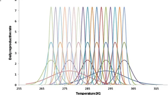
Niche overlap¼ðniche separation=niche spreadÞ ¼ðm1m2Þ=s The examined temperature range corresponds to the temperature variation in the temperate zone. Thirty-three algae species with various temperature sensitivity can be seen in the Fig.1. The daily reproductive rate of the species can be seen on the vertical axis, which means by how many times the number of specimens can increase on a given temperature. This corresponds to the reproductive ability of freshwater algae in the temperate zone [4,18,20].
The 33 species are described by the Gaussian distribu- tion with the following parameters:
& two super generalists (μSG1= 277 K; μSG2=293 K;
σSG=8.1)
& five generalists (μG1=269 K;μG2=277 K;μG3=285 K;
μG4=293 K;μG5=301 K;σG=3.1)
& nine transitional species (μT1=269 K; μT2=273 K;
μT3=277 K; μT4=281 K; μT5=285 K; μT6=289 K;
μT7=293 K;μT8=297 K;μT9=301 K;σT=1.66)
& 17 specialists (μS1=269 K; μS2=271 K; μS3=273 K;
μS4=275 K; μS5=277 K; μS6=279 K; μS7=281 K;
μS8=283 K; μS9=285 K; μS10=287 K; μS11=289 K;
μS12=291 K; μS13=293 K; μS14=295 K; μS15=297 K;
μS16=299 K;μS17=301 K;σS=0.85)
Since the reproductive ability is given, the daily number of specimens related to the daily average temperature is definitely determinable. We suppose 0.01 specimens for every species as starting value and the following minimum function describes the change in the number of specimens:
N Xð Þi 1¼0:01 for everyi¼1;2;. . .;33 species;
whereN(Xi): the number of specimens of the ith species
N Xð Þij¼N Xð Þi j1Min RRð ÞXij;a
1
P33
i¼1 N Xið Þ
Kj
0
@ 1 A 0 n
B@
1 CA 8 r
>>
>>
>>
><
>>
>>
>>
>:
9>
>>
>>
>>
=
>>
>>
>>
>; þ0:01;
where
j: is the number of the days (normallyj=1,2,…,3,655) RR(Xi)j: is the reproductive rate of theXispecies on the jth day
a=8 V=0.8
r: is the velocity parameter (r=1 or 0.1) Kj¼d1sinðd2kþd3Þþ
d4þ100;000RndðÞ 50;000, this is the restrictive function of reaching the sunlight.
k=1,2,…,366; this is the sequential number of the given year (year-day)
d1=4,950,000,d2=0.0172,d3=1.4045,d4=5,049,998 The constant values of theKjrestrictive function are set in a way where the period of the function is 365.25, the maximum place is on 23rd June, and the minimum place is on 22nd December (these are the most and the least sunny days).
In our researches, the distribution of the algae commu- nity of a theoretical freshwater ecosystem is examined by changing the temperature. Rivalry begins among the species with the change of temperature. In every tempera- ture interval, there are dominant species which win the competition. The temperature was changed according to plan in order to estimate the various effects separately. The duration of the simulation was usually 10 years in the experiments. Two experiment series were run according to the dual value of the velocity parameter.
The output parameters of the experiments are the determination of dominant species, the biggest number of specimens, the first year of the equilibrium and the usage of resources. Usage of the resources shows how much is utilised from the available resources (in this case, from sunlight) during the increase of the ecosystem.
Daily temperature values were calculated according to various functions. Simulations were made from the simplest case to the more complex exercise to explain harder questions, too. For the first time, the effect of the constant
temperature was examined on the change of the composi- tion of the theoretical ecosystem then the consequences of the linear increase in temperature for the number of species.
The annual fluctuation in temperature is periodic—it changes approximately according to the sine function; this sine temperature pattern is examined in the third series of the experiments.
We have found that the difference in temperature between the consecutive days ranges between −7 and 7 values with normal distribution. In order to simulate the daily temperature data, the fluctuation was made by random numbers (from ±1° to ±12°).
Finally, the effect of existing climate patterns (historical or future daily temperatures) was analysed where temperature values were from various climatic zones. Daily average temperature data are periodic through years; therefore, appropriate functions were made to describe the climate.
3 Describing the Temperature Function used during the Experiments
1. Constant temperature
Simulation experiments were made on 293, 294 and 295 K with the two velocity parameters (r=1 and 0.1).
Fluctuation was added as ±1…±11 K random numbers.
2. Linear increase in temperature for 10 years TðtÞ ¼T tð 1Þ þb;
where T(1) = 268 K is the temperature of the first day, t= 2,…,3,655 means the number of the days, β is the sensitivity, which changes from 0.0001 to 0.01.
Fig. 1 Reproductive temperature pattern of 33 algae species
3. Sine temperature pattern in a year
Annual average temperature of Budapest is about 283–
284 K (between 1960 and 1990); the range of temperature data is between 30 and 45 K. The following function describes this temperature pattern (with a day period of 365.25):
T¼s1sinðs2tþs3Þ þs4;
wheres2=0.0172,s3=−1.4045. During the experiments, the height (s1) and the place (s4) of the sine function can be modified. Thes1value is between 15 and 22.5 K, ands4is equal to 284 K according to the Budapest historical data.
4. Existing climate patterns (historical and future) One of the parameters used for describing the climate is the daily average temperature value. This means a great deal of numbers for long-term (30 years) examinations: 30×365 values. In order to simplify the description of the climate and to ignore the fluctuation between years, a function has been fitted to averages and dispersion of the 30 years’ data according to the least squares method. It is found that the daily average temperature from various climate zones fluc- tuates according to the following function (deterministic term):
TðtÞ ¼a1sinða2tþa3Þ þa4þa5sinða6tþa7Þ
The standard deviation of the daily average temperature during the 30 years can be described by the next function (stochastic term):
sðtÞ ¼b1sinðb2tþb3Þ þb4
The daily average temperature values can be classified according to their origin: historical or future. For these data series, daily temperature values can be generated with the following expression:
GeneratedðtÞ ¼averageðtÞ þð3:5RndðÞ 1:75Þ sðtÞ wheretis the number of the year,Rnd() is a random value between 0 and 1.
The classification of the used existing climate patterns is the following:
1. Historical temperature values from 1960 to 1990 in Hungary (Budapest, Debrecen, Győr, Pécs, Szeged) 2. Historical international data from various climate zones
(according to Köppen-Geiger classification, [14,15]) Daily average temperature data were collected with the help of web database [12] from the following cities all over the world (in some meteorological stations, there were not any available historical data for 30 years, only from 1995 to 2008):
(a) Tropical climate (Bangui 4°22′N 18°35′E, Central African Republic)
(b) Dry climate (Taskent 35°16′15″ N, 33°23′30″ E, Cyprus)
(c) Temperate climate (Den Helder 51°25′60″N, 4°31′ 60″E, The Netherlands)
(d) Continental climate (Ulan Bator 47°55′0″ N, 106°
55′0″E, Mongolia)
(e) Polar climate (Sodankyla, 67°25′00″ N, 26°35′35″
E, Finland)
A place has been chosen from the main climate zones and the change in the composition of our theoretical ecosystem has been examined.
3. Future temperature patterns from 2070 to 2100 in Hungary:
(a) Hadley Center adhfa (Regional Model 3, SRES A2) (b) Hadley Center adhfd (Regional Model 3, SRES B2) (c) MPI 3009
(d) GF2534 (e) GF5564 (f) UKLO
4. Analogous places in Hungary by 2100 [8]
It is predicted that the climate in Hungary will become the same which is the present day climate on the border of Romania and Bulgaria or near Thessaloniki. According to the worst prediction, the climate will be like the current North-African climate. Therefore, the following places have been examined:
(a) Turnu Magurele, Romania (43.75° N, 24.88° E, 31.0 m)
(b) Cairo, Egypt (30.058° N, 31.229° E)
Scenarios of analogue places are simple because tem- perature is the only factor which has been considered.
4 Results
1. Constant temperature
(a) r=1 (velocity factor); without daily fluctuation The ecosystem answers according to our expectations on constant temperature. The use of resources is nearly 100%.
293 K is the optimum reproductive temperature for the species S13, T7, G4 and SG1. Considering their amount, these species occur in the above sequence, but species G4 and SG1 have less than 100 specimens; 295 K is the optimum reproductive temperature for the species S14. The use of resources is almost 100%. During the simulation, the species S14 occurs with many, the other species (K7, K8, G4, SG1) with a few, less than 10 specimens.
There is no optimum reproductive temperature for any other species. In this case, the use of resources is nearly
100%; the species S13 and S14 have the same number of specimens (for both, five million specimens is the maxi- mum), and the species T7 reaches nearly one million specimens during the experiment.
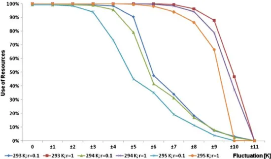
(b) r=1 (velocity factor); with daily fluctuation Changing the random fluctuation from ±1 to ±10 K, it is found that the use of resources decreases strongly in case of a fluctuation bigger than ±8 K.
(c) r=0.1 (velocity factor); with and without daily fluctuation
During these slower experiments, the value of the use of resources strongly decreases due to smaller fluctuation.
Comparing the cases of the constant temperature simulation, the results can be seen in Fig. 2, where the degree of the fluctuation is shown on the horizontal and that of the use of resources on the vertical axis.
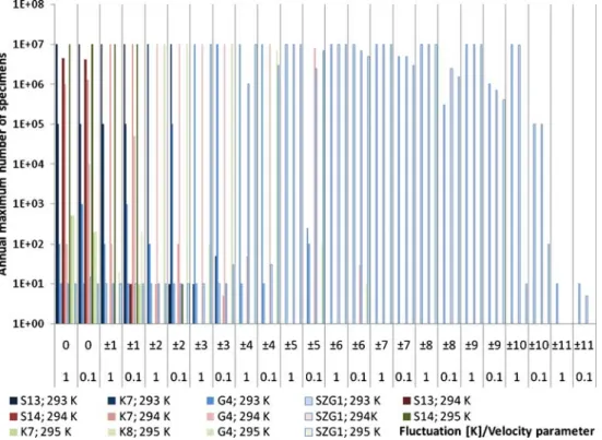
In Fig. 3, the maximum numbers of specimens are represented according to the experiments for 293, 294 and 295 K, respectively. Within a year, the number of speci- mens usually fluctuates in two orders of magnitude since there is a restriction for reaching the sunlight. The darkest colours show the specialists; apparently, these species occur in experiments with little fluctuation. Decreasing the velocity factor, the specialists also occur in case of larger random numbers. The transient species are followed by the generalists as the colours are fading on the diagram. The lightest super generalist is the only one above ±6 K fluctuation, and it reaches the maximum fluctuation where it is able to reproduce (±10 K).
The time of reaching the dynamic equilibrium can be seen in Fig. 4. Decreasing the velocity factor, the
equilibrium evolves later: the reddish colours are related to slower, the bluish ones are related to faster processes.
2. Linear increase in temperature for 10 years
During these experiments, the sensitivity factor (β) was changed. The result can be seen in the Fig. 5, where the vertical axis shows the use of resources; the horizontal axis is related to sensitivity and fluctuation. The starting temperature value was 268 K in all cases. The slower processes have smaller values for the use of resources as it can be seen in cases of constant temperature as well.
In case of processes that have had larger sensitivity (β= 0.005 or 0.01), the use of resources does not decrease to zero in case of quite large random fluctuation (±7 K) as it does in cases with smaller sensitivity.
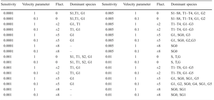
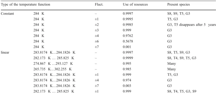
The dominant species for each experiment can be seen in Table 1. The increase of the fluctuation is good for the super generalists.
Comparing the constant and the linear cases around 284 K, there is no species which would have this temperature as an optimum reproductive value (see Table2).
In cases where there is no fluctuation, the specialists occur but when there is a little increase in fluctuation, these specialists disappear.
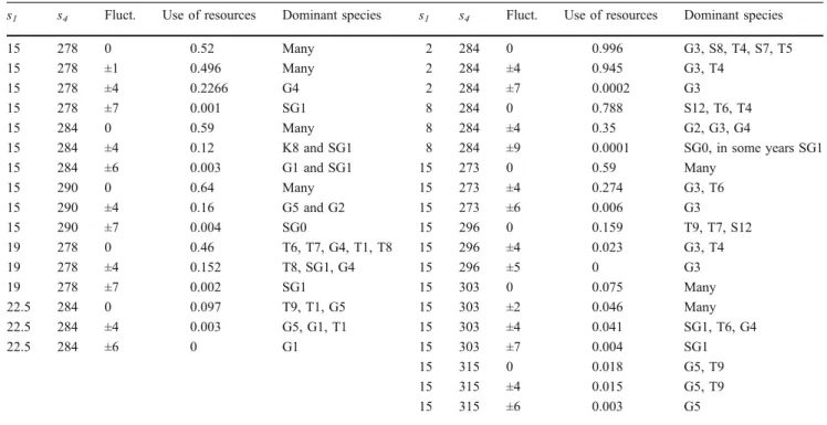
3. Sine temperature pattern within a year
The sine function of the annual temperature pattern has two changeable parameters. One of these is the parameters1: this means the height of the amplitude of the function; the other is the parameter s4, which shows the annual average temperature. Increasing the amplitude (s1) of the function, values of the use of resources significantly decrease. The increase in random fluctuation makes the use of resources
Fig. 2 Use of resources values for various velocity parameters on constant temperature
values decrease (see Fig.6). The dominant species and the values of the use of resources can be seen in Table3.
Doing the simulation series, in case of smaller velocity parameter (r=0.1), it is found that the use of resources is nearly zero almost in all without-fluctuation cases. There are two cases when the use of resources values are not equal to zero, with s1=2 and s4=284 parameters it becomes 0.924 without fluctuation and 0.7856 with ±4 K fluctuation. In the second case, the parameters ares1=8,s4=284, and the use of resources becomes 0.0115 without any fluctuation. The distribution of species largely differs according to velocity.
4. Temperature values from 1960 to 1990 in Hungary The equilibrium has been reached; the competition of the species can be seen in Fig.7. The faster ecosystem has a lot of specialists and some transient species. During summer, there is stationary temperature; therefore, the slower and the faster ecosystems show quite a similar picture (species S13, T7, G4 and SG1); in winter, the species K2 (the lightest) occurs.
5. (a) Future temperature in Budapest
According to the A2 scenario (HC adhfa), there is no optimum reproductive temperature for any species during Fig. 4 The year of reaching
the dynamic equilibrium during simulations with constant temperature and increasing fluctuation
Fig. 3 Annual maximum num- ber of specimens of the species on constant temperature with different velocity parameters (logarithmic representation)
the slower or the faster processes. In winter, there will be more species such as G2, T3, S5 and S6. According to the B2 scenario (HC adhfd), the species G5 has optimum reproductive temperature in summer.
(b) Future temperature in Debrecen
Viewing the results of various temperature data series of Debrecen, there is no difference from the results of Budapest.
There are older predictions for the future temperature in Debrecen (UKLO, UKTR31, GF2534, GF5564, UKTR31),
which show similar results with the historical data series.
The UKLO estimation resembles the MPI 3009 prediction as the seasons do not separate. The results of this prediction considerably differ from the other data series, the species S16, T9 and T8 occur in summer.
Comparing the UKHI and UKLO predictions, the results differ. In the first case, there is no separation between the seasons; in the second, one summer and winter are well separated. The occurring species considerably differ from the results of the newer predictions (MPI, HC).
Table 1 Dominant species in experiments having linear increase in temperature
Sensitivity Velocity parameter Fluct. Dominant species Sensitivity Velocity parameter Fluct. Dominant species
0.0001 1 0 S1,T1, G1 0.005 1 0 S1–S8, T1–T4, G1, G2
0.0001 0.1 0 S1,T1, G1 0.005 0.1 0 S1–S8, T1–T4, G1, G2
0.0001 1 ±2 G1, T1 0.005 1 ±2 T1–T4, G1–G3
0.0001 0.1 ±2 T1, G1 0.005 0.1 ±2 T1–T4, G1–G3
0.0001 1 ±5 G1 0.005 1 ±5 G1, SG0, G3
0.0001 0.1 ±5 G1 0.005 0.1 ±5 G1, SG0, G2,G3
0.0001 1 ±8 – 0.005 1 ±8 SG0
0.0001 0.1 ±8 – 0.005 0.1 ±8 SG0
0.001 1 0 S1, T1, S2, G1 0.01 1 0 S, T,G
0.001 0.1 0 S1, T1, S2, G1 0.01 0.1 0 S, T,G
0.001 1 ±2 T1, G1 0.01 1 ±2 T1–T8, G1–G5
0.001 0.1 ±2 T1, G1 0.01 0.1 ±2 T1–T8, G1–G5
0.001 1 ±5 G1 0.01 1 ±5 G1, SG0, SG1, G5
0.001 0.1 ±5 G1 0.01 0.1 ±5 G1, G2, SG0, G4, SG1, G5
0.001 1 ±8 – 0.01 1 ±8 SG0, SG1
0.001 0.1 ±8 – 0.01 0.1 ±8 SG0, SG1
Fig. 5 Use of resources values for various velocity parameters in case of linear temperature patterns and a few types of fluctuation
6. Analogous places in Hungary by 2100
The simulation results of analogous places show that the species composition is similar to the historical data in case of Turnu Magurele, similarity exists with future estimations in winter. Present-day temperature of Cairo shows analogy with MPI 3009 predictions by 2070–2100 rather well.
7. Historical international data from various climate zones Bangui is situated in the tropical zone; therefore, the temperature is nearly constant throughout the year. In this climate, the species G5 is autocrat. In case of slower
process, the specialist S16 occurs among the dominant species:
Taskent has dry, waste climate, where the species pattern is similar to the future predictions for 2100 in Hungary.
In Den Helder, the seasons separate well.
In Sodankyla, species which have cold tolerance except in winter can reproduce.
In Addis Ababa, the species SG1 becomes dominant in the course of the faster case; during the lower simulation, the dominant species are G4, K6 and S12.
Table 2 Examinations at an average temperature of 284 K in several experiments
Type of the temperature function Fluct. Use of resources Present species
Constant 284 K – 0.9997 S8, S9, T5, G3
284 K ±1 0.9995 T5, G3
284 K ±2 0.9985 G3, T5 disappears after 5 years
284 K ±3 0.999 G3
284 K ±4 0.9762 G3
284 K ±6 0.5678 G3
284 K ±7 0.001 G3
linear 283.8174 K…284.1826 K – 0.9997 S8, T5, S9, G3
282.173 K…285.825 K – 0.9999 S8, T4, S9, T5, G3
274.867 K…293.127 K – 0.995 Many
265.735 K…302.255 K – 0.985 Many
283.8174 K…284.1826 K ±1 0.999 T5, G3
283.8174 K…284.1826 K ±4 0.974 G3
283.8174 K…284.1826 K ±7 0.003 G3
282.173 K…285.825 K ±1 0.999 S8, T4, T5, G3, S9
Fig. 6 Use of resources values in simulations with sine temperature patterns withr=1 velocity parameter
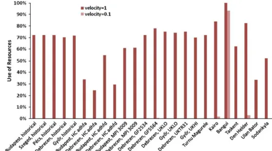
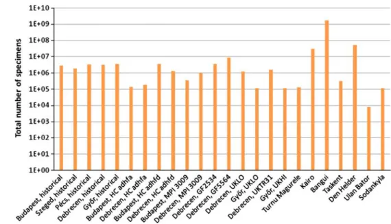
8. Comparisons
The use of resources values for the various simulations can be seen in Fig.7. The annual number of all specimens for simulations is shown in Figs.8,9 and10.
5 Conclusion
1. Analysing the results of constant temperature, it can be stated that the specialists and transient species adapted best to the given temperature are dominant during the competition, but generalists and super generalists occur rarely; the use of resources value is nearly 100%. Considering the random fluctuation,
some species disappear depending on the degree of the fluctuation. First, in case of a random temperature of ±1 K, specialists disappear in large amount, then also the transient species, and in case of a random fluctuation of ±5 K, only super generalists exist. It can be said that plants disappear in case of large (±10 K random numbers) temperature fluctuation.
2. Regarding the effect of the velocity factor, it can be stated that the equilibrium is established slower in case of slower simulation process; at least 10 years are needed to reach the equilibrium while only 1 year is enough in case of a simulation with a velocity factor equal to 1. For example, on 295 K with a fluctuation of ±4 K, only one species (SG1) exists after the first
1.E+00 1.E+01 1.E+02 1.E+03 1.E+04 1.E+05 1.E+06 1.E+07
1500 1550 1600 1650 1700 1750 1800 1850 1900 1950 2000
Total number of species
1.E+00 1.E+01 1.E+02 1.E+03 1.E+04 1.E+05 1.E+06 1.E+07
1500 1550 1600 1650 1700 1750 1800 1850 1900 1950 2000
Total number of species
Fig. 7 Total number of species related to the historical climate of Budapest forr=1 (left side) andr=0.1 (right side) velocity parameters during 400 days
Table 3 Results of the simulations according to sine temperature patterns
s1 s4 Fluct. Use of resources Dominant species s1 s4 Fluct. Use of resources Dominant species
15 278 0 0.52 Many 2 284 0 0.996 G3, S8, T4, S7, T5
15 278 ±1 0.496 Many 2 284 ±4 0.945 G3, T4
15 278 ±4 0.2266 G4 2 284 ±7 0.0002 G3
15 278 ±7 0.001 SG1 8 284 0 0.788 S12, T6, T4
15 284 0 0.59 Many 8 284 ±4 0.35 G2, G3, G4
15 284 ±4 0.12 K8 and SG1 8 284 ±9 0.0001 SG0, in some years SG1
15 284 ±6 0.003 G1 and SG1 15 273 0 0.59 Many
15 290 0 0.64 Many 15 273 ±4 0.274 G3, T6
15 290 ±4 0.16 G5 and G2 15 273 ±6 0.006 G3
15 290 ±7 0.004 SG0 15 296 0 0.159 T9, T7, S12
19 278 0 0.46 T6, T7, G4, T1, T8 15 296 ±4 0.023 G3, T4
19 278 ±4 0.152 T8, SG1, G4 15 296 ±5 0 G3
19 278 ±7 0.002 SG1 15 303 0 0.075 Many
22.5 284 0 0.097 T9, T1, G5 15 303 ±2 0.046 Many
22.5 284 ±4 0.003 G5, G1, T1 15 303 ±4 0.041 SG1, T6, G4
22.5 284 ±6 0 G1 15 303 ±7 0.004 SG1
15 315 0 0.018 G5, T9
15 315 ±4 0.015 G5, T9
15 315 ±6 0.003 G5
year in the faster simulation, but in the slower simulation, there are two species (G4 and SG1) with nearly equal number of specimens after 10 years.
3. Considering the values of the use of resources with change of fluctuation, it can be seen that in case of faster processes, this value is nearly 100% up to a random fluctuation of ±7 K, then it quickly breaks down. During the simulations with a velocity value of 0.1, the value of the use of resources gradually decreases from ±3 to 4 K random numbers.
4. If the temperature slowly changes according to a linear function, the specialists and transient species favouring the given temperature exist in the ecosys- tem. The super generalist occurs in very little amount in simulations with little fluctuations. As the fluctua- tion increases, only the super generalist will occur due to ±4 K random numbers.
5. Changing the parameters4in sine temperature pattern simulations, it can be seen that the use of resources is little on the border of the examined temperature interval (T=303 and 315 K). With increasing fluctu- ation, the species disappear when random numbers are larger than ±6 K. The parameter s1 stands for the amplitude of the sine functions; increasing this value, the values of the use of resources decrease.
6. As a general rule, it can be said that specialists disappear from dominant species in case of a fluctuation of already ±1 K. Generalists exist up to a daily fluctuation of ±6 to 7 K, but above these values, only super generalists occur up to a fluctuation of maximum ±10 to 11 K.
7. In case of sine temperature pattern, it can be stated that decreasing the value of the velocity factor, the number of specimens significantly decreases. Mean-
Fig. 9 Total number of specimens for a year in case of various climates withr=1 velocity parameter
Fig. 8 Use of resources values in case of various climate zones
while, the amplitude of the temperature function is quite small (s1=2 or 8); there are some specimens, but increasing the amplitude, the species disappear.
8. The total number of specimens in a year decreases for the given species in the future (using estimated weather data series by 2070–2100, MPI 3009, HC adhfa and HC adhfd), the degree of decrease is different among the various results.
9. The older predictions (UKLO, UKHI and UKTR31) show nearly the same values as historical results do related to the use of resources and the annual average number of specimens.
10. Comparing the Hungarian historical data with results of predictions of analogous places by 2100 (Cairo, Turnu Magurele), it can be said that the total number of specimens is the same, but it is a little higher in case of Cairo. During the slower simulation process, the total number of specimens decrease in case of Turnu Magurele, and in Cairo, there will be signifi- cantly more specimens (10 times more).
11. The artificial ecosystem reaches a dynamic equilibri- um in 2 to 3 years in case of the predicted and historical data series except for the slower simulation with constant temperature, where this period lasts for 7–10 years.
6 Discussion
In the course of our simulations, it has been shown what kind of effects there are on the composition and competi- tion of an ecosystem when temperature changes. Specialists reproducing in narrow temperature interval are dominant species in case of constant or slowly changing temperature
pattern, but these species disappear in case of small fluctuation in the temperature. Many authors draw attention to the relevance of temperature as the main regulating factor [2,3,19].
Changing climate means the increase not only in the annual average temperature but also in variability, which is a larger fluctuation among daily temperature data [5]. As a consequence, species with narrow adaptation ability disap- pear, species with wide adaptation ability become dominant and the biodiversity decreases.
Because of global warming and changing climate, the various ecosystems have to find a way to reach the equilibrium. Some plant species will disappear because of the change in optimum temperature, which is needed for their reproduction. The number of specimens could largely change and the composition of various ecosystems will be reorganised.
Comparing the Hungarian historical data with the regional predictions of huge climate centres (HC, MPI), it can be stated that the newer estimations (such as HC adhfa, HC adhfd and MPI 3009) show a decrease in the number of specimens in our theoretical ecosystem. According to the older predictions (such as UKLO, UKHI and UKTR31), the composition of the ecosystem does not change in propor- tion to the historical results.
In the predictions, places where the temperature is the same now as it will be in Hungary by 2100 are dealt with.
Simulations with the historical temperature pattern of these analogous places show that our ecosystem works similarly in the less hot Rumanian lowland (Turnu Magurele); the number of specimens and the use of resources increase using North African temperature data series. In further research, it could be interesting to analyse the differences in the radiation regime of the analogous places.
Fig. 10 Total number of speci- mens for a year in case of various climates withr=0.1 velocity parameter (logarithmic representation)
Ecosystems have an important role in the biosphere in development and maintenance of the equilibrium. Regard- ing the temperature patterns, it is not only the climate environment which affects the composition of ecosystems but plants also make a feedback to their milieu during the photosynthesis and respiration in the global carbon cycle.
Specimens of the ecosystems do not only suffer from change in climate but they can also affect the equilibrium of the biosphere or the composition of the air through the biogeochemical cycles. There is an opportunity to examine the controlling ability of temperature and climate with the theoretical ecosystem.
In our further research, we would like to examine the effect of the ecosystem on the climate. These temperature feedbacks have got a great emphasis related to DGVM models with large computation needs [7], but the feedbacks cannot be estimated directly. We would like to examine the process of the feedback with PC calculations to answer easy questions.
Acknowledgements This investigation was supported by the proj- ects NKFP 4/037/2001 and OTKA T042583, the VAHAVA project, the Adaptation to Climate Change Research Group of the Hungarian Academy of Sciences and the Department of Mathematics and Informatics, Corvinus University of Budapest.
References
1. Baranovic, A., Solic, M., Vucetic, T., & Krstulovic, N. (1993).
Temporal fluctuations of zooplankton and bacteria in the middle Adriatic Sea.Marine Ecology Progress Series, 92, 65–75.
2. Dippner, J. W., Kornilovs, G., & Sidrevics, L. (2000). Long-term variability of mesozooplankton in the Central Baltic Sea.Journal of Marine Systems, 25, 23–31.
3. Dregelyi-Kiss, A., & Hufnagel, L. (2009). Simulations of Theoretical Ecosystem Growth Model (TEGM) during various climate conditions.Applied Ecology and Environmental Research, 7(1), 71–78.
4. Felföldy, L. (1981).A vizek környezettana. Általános hidrobioló- gia. Budapest: Mezőgazdasági Kiadó. Water environmental sciences.
5. Fischlin, A., Midgley, G. F., Price, J. T., Leemans, R., Gopal, B., Turley, C., et al. (2007). Ecosystems, their properties, goods, and services. In M. L. Parry, O. F. Canziani, J. P. Palutikof, P. J. van der Linden, & C. E. Hanson (Eds.), Climate change 2007:
impacts, adaptation and vulnerability. Contribution of working group ii to the fourth assessment report of the intergovernmental
panel on climate change(pp. 211–272). Cambridge: Cambridge University Press.
6. Foley, J. A., Prentice, I. C., Ramankutty, N., Levis, S., Pollard, D., Sitch, S., et al. (1996). An integrated biosphere model of land surface processes, terrestrial carbon balance, and vegetation dynamics.Global Biogeochemical Cycles, 10, 603–628.
7. Friedlingstein, P., Cox, P. M., Betts, R. A., Bopp, L., von Bloh, W., Brovkin, V., et al. (2006). Climate-Carbon Cycle feedback analysis:
Results from the C4MIP model incomparison.J. Climate, 19, 3337–
3353.
8. Hufnagel, L., Sipkay, C. S., Drégelyi-Kiss, Á., Farkas, E., Türei, D., Gergócs, V., et al. (2008). Klímaváltozás, Biodiverzitás és közösségökológiai folyamatok kölcsönhatásai. In Z. S. Harnos &
L. Csete (Eds.), Klímaváltozás: Környezet-Kockázat-Társadalom (pp. 275–300). Budapest: Szaktudás Kiadó Ház.
9. Juhász-Nagy, P. (1984).Beszélgetések az ökológiáról. Budapest:
Mezõgazdasági Kiadó. Conversation about ecology.
10. Juhász-Nagy, P. (1986).Egy operatív ökológia hiánya, szükséglete és feladatai(p. 251). Budapest: Akadémiai Kiadó.
11. Juhász-Nagy, P. (1993).Az eltűnõ sokféleség (A bioszféra-kutatás egy központi kérdése). Budapest: Scientia Kiadó.
12. Klein Tank, A. M. G., & Coauthors. (2002). Daily dataset of 20th- century surface air temperature and precipitation series for the European Climate Assessment. International Journal of Clima- tology, 22, 1441–1453.
13. Parmesan, C., et al. (1999). Poleward shifts in geographical ranges of butterfly species associated with regional warming. Nature, 399, 579–583.
14. Péczeli, G. (1981). Éghajlattan (pp. 239–257). Budapest:
Tankönyvkiadó.
15. Peel, M. C., Finlayson, B. L., & McMahon, T. A. (2007). Updated world map of the Köppen-Geiger climate classification. Hydrol.
Earth Syst. Sci., 11, 1633–1644.
16. Pianka, E. R. (1974). Niche overlap and diffuse competition.
Proc. Nat. Acad. Sci. U. S. A., 71(5), 2141–2145.
17. Précsényi, I. (1995). Alapvetõ kutatásszervezési, statisztikai és projectértékelési módszerek a szupraindividuális biológiában.
Debrecen: KLTE.
18. Reynolds, C. (2006). Ecology of phytoplankton. Cambridge:
Cambridge University Press.
19. Sipkay, C. S., Hufnagel, L., Révész, A., & Petrányi, G. (2007).
Seasonal dynamics of an aquatic macroinvertebrate assembly (Hydrobiological case study of Lake Balaton No. 2). Applied Ecology and Environmental Research, 5(2), 63–78.
20. Sipkay, C., Horváth, L., Nosek, J., Oertel, N., Vadadi-Fülöp, C., Farkas, E., et al. (2008). Analysis of climate change scenarios based on modelling of the seasonal dynamics of a Danubian copepod species.Applied Ecology and Environmental Research, 6 (4), 101–108.
21. Spellerberg, I. F. (1991). Monitoring ecological change. Cam- bridge: Cambridge University Press.
22. Vadadi-Fülöp, C. S., Türei, D., Sipkay, C. S., Verasztó, C. S., Dregelyi-Kiss, A., & Hufnagel, L. (2008). Comparative assessment of climate change scenarios based on aquatic food web modelling.
Environmental Modelling and Assessment, 14(5), 563–576.