1
This is the final accepted version of the article (DOI:10.1016/j.ecolind.2017.11.012). The final published version can be found at
https://www.sciencedirect.com/science/article/pii/S1470160X17307240
Title: Evaluating and benchmarking biodiversity monitoring: metadata-based indicators for sampling design, sampling effort and data analysis
Authors: Szabolcs LENGYELa*, Beatrix KOSZTYIa, Dirk S. SCHMELLERb, Pierre-Yves HENRYc, Mladen KOTARACd, Yu-Pin LINe and Klaus HENLEb
Affiliations:
a Department of Tisza Research, Danube Research Institute, Centre for Ecological Research, Hungarian Academy of Sciences, Bem tér 18/c, 4032 Debrecen, Hungary; Emails:
lengyel.szabolcs@okologia.mta.hu (SL), cleo.deb@gmail.com (BK)
b Helmholtz Centre for Environmental Research − UFZ, Department of Conservation Biology, Permoserstr. 15., Leipzig, D-04318, Germany; Email: dirk.schmeller@ufz.de (DSS), klaus.henle@ufz.de (KH)
c Centre d’Écologie et des Sciences de la Conservation (CESCO UMR 7204), CNRS, MNHN, UPMC, Sorbonne Universites & Mecanismes Adaptatifs et Evolution (MECADEV UMR 7179), CNRS, MNHN, Sorbonne Universites, Muséum National d’Histoire Naturelle, 1 avenue du Petit Château, 91800, Brunoy, France; Email: henry@mnhn.fr
d Centre for the Cartography of Fauna and Flora, Kunova ulica 3, SI-1000, Ljubljana, Slovenia; Email: mladen@ckff.si
e Department of Bioenvironmental Systems Engineering, National Taiwan University, Taipei 10617, Taiwan; Email: yplin@ntu.edu.tw
Correspondence:
* SL, Phone: +36 (52) 509-200/11635 (office), +36 (30) 488-2067 (mobile); Email:
lengyel.szabolcs@okologia.mta.hu
Running title: Benchmarking biodiversity monitoring
Word count: 6966
Abstract with keywords: 262 Main text: 4914
Acknowledgements and Data accessibility: 84 Tables: 562
Figure legends: 180 References: 864
Number of tables: 3, number of figures: 6 Number of references: 33
2
ABSTRACT
1
1. The biodiversity crisis has led to a surge of interest in the theory and practice of
2
biodiversity monitoring. Although guidelines for monitoring have been published since the
3
1920s, we know little on current practices in existing monitoring schemes.
4
2. Based on metadata on 646 species and habitat monitoring schemes in 35 European
5
countries, we developed indicators for sampling design, sampling effort, and data analysis to
6
evaluate monitoring practices. We also evaluated how socio-economic factors such as starting
7
year, funding source, motivation and geographic scope of monitoring affect these indicators.
8
3. Sampling design scores varied by funding source and motivation in species monitoring and
9
decreased with time in habitat monitoring. Sampling effort decreased with time in both
10
species and habitat monitoring and varied by funding source and motivation in species
11
monitoring.
12
4. The frequency of using hypothesis-testing statistics was lower in species monitoring than
13
in habitat monitoring and it varied with geographic scope in both types of monitoring. The
14
perception of the minimum annual change detectable by schemes matched spatial sampling
15
effort in species monitoring but was rarely estimated in habitat monitoring.
16
5. Policy implications: Our study identifies promising developments but also options for
17
improvement in sampling design and effort, and data analysis in biodiversity monitoring. Our
18
indicators provide benchmarks to aid the identification of the strengths and weaknesses of
19
individual monitoring schemes relative to the average of other schemes and to improve
20
current practices, formulate best practices, standardize performance and integrate monitoring
21
results.
22 23 24
3
KEYWORDS
25
2020 target; assessment; biodiversity observation network; biodiversity strategy; citizen
26
science; conservation funding; environmental policy; evidence-based conservation; statistical
27
power; surveillance
28 29
1. INTRODUCTION
30
The global decline of biodiversity and ecosystem services led to the adoption of several
31
ambitious goals by the international community for 2010 and then again for 2020. Monitoring
32
of biodiversity is instrumental in evaluating whether these goals are met. Although literature
33
on how monitoring systems should be organized has been published since at least the mid-
34
1920s (Cairns and Pratt, 1993), interest in the theory and practice of biodiversity monitoring
35
has surged since 1990 (Noss, 1990; Yoccoz et al., 2001) and culminated in comprehensive,
36
theory-based recommendations for monitoring (Balmford et al., 2003; Lindenmayer and
37
Likens, 2009; Mace et al., 2005; Pocock et al., 2015).
38 39
Despite this growing knowledge, significant concerns regarding current practices remain
40
(Lindenmayer and Likens, 2009; Walpole et al., 2009). A consistently voiced concern is that
41
monitoring is not adequately founded in theory because many schemes are not designed to
42
test hypotheses about biodiversity change even though their primary objective, almost
43
exclusively, is to detect changes in biodiversity (Balmford et al., 2005; Nichols and Williams,
44
2006; Yoccoz et al., 2001). Although not all monitoring schemes require hypothesis-testing
45
given the variety of their objectives (Pocock et al., 2015), there is also a general concern over
46
the ability of monitoring schemes to adequately detect changes in biodiversity due to biased
47
sampling designs, inadequate sampling effort, or low statistical power to detect changes (Di
48
Stefano, 2001; Mihoub et al., 2017). Legg & Nagy (2006) and Lindenmayer & Likens (2009)
49
4
warned that these shortcomings may lead to poor quality of monitoring, and, ultimately, to a
50
waste of valuable conservation resources.
51 52
There is little information, however, on the prevalence of these potential methodological
53
weaknesses in current practices of biodiversity monitoring. Descriptions of current practices
54
are available for monitoring schemes in North America (Marsh and Trenham, 2008), and for
55
European schemes of habitat monitoring (Lengyel et al., 2008a) and bird monitoring
56
(Schmeller et al., 2012), however, these descriptions do not evaluate strengths or weaknesses
57
in monitoring. Monitoring schemes are rarely known well enough for a comprehensive
58
evaluation of current practices (Henle et al., 2010a; Schmeller et al., 2009), partly because
59
monitoring schemes are designed for many different objectives at different spatial and
60
temporal scales (Geijzendorffer et al., 2015; Jarzyna and Jetz, 2016; Pocock et al., 2015).
61
Therefore, the performance of biodiversity monitoring in terms of the criteria regarded by the
62
critiques as insufficiently considered in monitoring has not yet been assessed. Consequently,
63
little is known about whether and how performance varies among programs by spatial and
64
temporal scales or socio-economic drivers. Moreover, it is rarely known whether and how
65
programs evaluate their performance, either by expert judgement on their ability to detect
66
trends or by estimating their statistical power to detect changes (Geijzendorffer et al., 2015;
67
Nielsen et al., 2009). Hence, there is a need to provide monitoring coordinators with standard
68
indicators of performance so that they can evaluate their programs and revise their practices
69
to address potential weaknesses. A clear understanding of performance in existing monitoring
70
schemes also provides crucial information to the institutions running and funding monitoring
71
schemes as well as to policy-makers using information from biodiversity monitoring.
72 73
5
Here we present an overview of current practices in biodiversity monitoring in Europe by
74
focusing on properties that have been frequently mentioned in critiques of biodiversity
75
monitoring. We used metadata on monitoring schemes to develop indicators for sampling
76
design, sampling effort and type of statistical analysis. While monitoring schemes have been
77
established for many different purposes, these three properties are regarded as generally
78
relevant in determining the scientific quality of the information derived from biodiversity
79
monitoring (Lindenmayer and Likens, 2009; Nichols and Williams, 2006; Yoccoz et al.,
80
2001). Sampling design, an indicator of how well the spatial and temporal distribution of data
81
collection is founded in sampling theory (Balmford et al., 2003), is essential for accuracy,
82
i.e., closeness of measured trends and real trends in biodiversity. Sampling effort, the number
83
of measurements made, is central to precision, i.e., the ability to measure the same value
84
under identical conditions. Finally, to translate collected data into information relevant for
85
further use, such as conservation or policy, appropriate statistical analysis of data is required
86
to detect changes or trends with a given level of uncertainty, and confidence in the estimates
87
should be based on the ability of the scheme to detect changes (Legg and Nagy, 2006).
88 89
Although these three indicators are generally relevant in any type of monitoring, monitoring
90
schemes differ in their objectives and many different types of monitoring schemes exist
91
(Pocock et al., 2015). For example, schemes in Europe have been started as early as the
92
1970s, are motivated by different reasons, funded by different sources, and their geographic
93
scope ranges from local to continental (Lengyel et al., 2008a; Schmeller et al., 2012). To
94
account for these socio-economic differences and to increase the useability of our indicators
95
in different monitoring schemes, we evaluated the variation in indicators as a function of
96
starting year, funding source, motivation, and geographic scope. Finally, we show how our
97
indicators can be used by coordinators as benchmarks to assess their schemes relative to the
98
6
average practice and to identify options for improvement of their monitoring schemes. We
99
present different benchmark values for the three indicators to be meaningful for schemes
100
monitoring different species groups and habitat types.
101 102
2. METHODS
103
2.1. Definition and dataset
104
We used Hellawell’s (1991) definition of “biodiversity monitoring” as the repeated recording
105
of the qualitative and/or quantitative properties of species, habitats, habitat types or
106
ecosystems of interest to detect or measure deviations from a predetermined standard, target
107
state or previous status in biodiversity. We collected metadata on biodiversity monitoring
108
schemes in Europe in an online survey (Henle et al., 2010a). The online questionnaire
109
contained 8 general questions and 33 and 35 specific questions on species and habitat
110
monitoring schemes, respectively (Table S1, S2). We sent more than 1600 letters with
111
requests to fill out the questionnaire to coordinators of monitoring schemes, government
112
officials, national park staff, researchers and other stakeholders at institutions involved in
113
biodiversity monitoring. The information entered was quality-checked and organized into a
114
meta-database (http://eumon.ckff.si/monitoring).
115 116
The survey response rate was 40% (646 schemes for 1600 letters), which was comparable to
117
the only other questionnaire-based study of biodiversity monitoring (48%) (Marsh and
118
Trenham, 2008). Response rate varied among countries and we evaluated this bias based on
119
the logic of Schmeller et al. (2009) (Supporting Information S1.1). Our metadatabase is
120
not, and cannot be, exhaustive to involve all monitoring schemes because the universe of all
121
schemes is not known, however, it provides a cross-section of geographic scope (Supporting
122
Information S1.1). The final dataset contained metadata on 470 species schemes and 176
123
7
habitat schemes, or a total of 646 schemes from 35 countries in Europe. Assessment of
124
country bias showed no substantial differences from the usual publication bias for 25 (or
125
71%) of the 35 countries, overrepresentation for three countries and underrepresentation for
126
seven countries (Fig. S1).
127 128
2.2. Indicator development
129
To compute an indicator of sampling design, we scored seven design variables in both
130
species and habitat monitoring schemes (Table 1). Scores were chosen to be higher for
131
sampling designs that were better founded in sampling theory and/or that obtained more or
132
better, e.g. quantitative rather than qualitative, information on species and habitats (further
133
details: Supporting Information S1.3). Scores were determined for each scheme as a
134
consensus among DSS, KH and SL. As a final output, we calculated a ‘sampling design
135
score’ (SDS) indicator as the sum of the seven scores (range: 0-13 in species schemes, 0-10 in
136
habitat schemes).
137 138
For sampling effort, we derived both a temporal and a spatial indicator. We used the
139
following formula for the “temporal sampling effort” indicator:
140 141
SEtemp = log(Fby(T2 − 1)(T*Fwy − 2)), (eqn 1)
142 143
where Fby is the between-year frequency of sampling (value of 1 indicating monitoring in
144
every year, 0.5 for monitoring every other year, etc.); T is the duration of monitoring in years;
145
and Fwy is the number of sampling occasions (site visits) within a year. A derivation of
146
equation 1 is given in Supporting Information S1.4.
147 148
8
For the “spatial sampling effort” indicator (SEspatial), we used information on the number of
149
sampling sites and the total area monitored. Assuming that more sampling sites in equal-sized
150
areas indicate higher sampling effort, we calculated the residuals from an ordinary least-
151
squares regression of the number of sites (log-transformed response) over the total area
152
monitored (log-transformed predictor). Positive values (above the fitted line) indicate higher-
153
than-average effort, whereas negative values (below the fitted line) indicate lower-than-
154
average effort for equal-sized areas.
155 156
Each of these three indicators (SDS, SEtemp, SEspatial) is negatively proportional to at least one
157
source of variation (temporal, among-site, or within-site) that increases the variance of the
158
trend estimate from monitoring. Hence the higher the values of the indicators, the better the
159
sampling design, the higher the sampling effort, and the higher the precision of the trend
160
estimate. The three indicators cannot be readily integrated but have the advantage that
161
coordinators of monitoring schemes can easily calculate them based on Eq. (1) or the
162
regression equations and can use them as benchmarks (see Results).
163 164
For the “type of data analysis” indicator, we used information on the analytical method as
165
given by the coordinators. The single-choice options were (i) descriptive statistics or
166
graphics, (ii) simple linear regression, (iii) advanced statistics, e.g. general linear models etc,
167
(iv) other analyses, (v) data analyzed by somebody else, or (vi) data not analyzed. We
168
considered options (i) and (vi) as evidence for the lack of inferential statistics and hypothesis-
169
testing and considered all other options as signals for hypothesis-testing.Although the option
170
‘data analyzed by someone else’ could also involve descriptive statistics or graphics, i.e., no
171
hypothesis-testing, this option was chosen for only 26 species schemes (<6% of 439
172
9
responses) and four habitat schemes (<3% of 154 responses), and pooling these into either
173
group did not influence our results.
174 175
Finally, to evaluate the coordinators’ expert judgement of the ability of their schemes to
176
detect changes, we asked coordinators to estimate the precision of their scheme as the
177
minimum annual change per year in the monitored property (e.g. population size, habitat
178
area) that is detectable by their scheme (1%, 5%, 10%, 20%, or more). We then correlated
179
these “precision estimates” with our temporal and spatial indicators of sampling effort to test
180
whether coordinators correctly estimated the sampling effort of their schemes. We arbitrarily
181
took 30% for responses of ‘more than 20%’. We found that using different percentages (40%,
182
50% etc.) did not qualitatively affect our conclusions.
183 184
2.3. Socio-economic effects
185
We analyzed the variation in each indicator caused by four socio-economic factors: (i)
186
starting year, (ii) main funding source (European Union [EU], national, regional, scientific
187
grant, local), (iii) motivation (EU directive, other international law, national law,
188
management/restoration, scientific interest, other), and (iv) geographic scope (pan-European,
189
international, national, regional, local). These factors were chosen because they are
190
fundamentally important in biodiversity monitoring and because knowledge of how these
191
factors impact the indicators (e.g. “sampling designs are more advanced in schemes funded
192
by certain types of donors”) will influence how monitoring coordinators and institutions
193
interpret and use the indicators.
194 195
To detect changes in certain time periods, we classified schemes by starting year in four time
196
periods of European biodiversity policy: (i) period 1: years until the adoption of the Birds
197
10
Directive in 1979, (ii) period 2: from 1980 until the adoption of the Habitats Directive in
198
1992, (iii) period 3: 1993 until 1999, and (iv) period 4: since 2000 or the preparations of the
199
2010 biodiversity targets. For funding source, motivation, and geographic scope, we used the
200
single-choice responses as given by the coordinators.
201 202
2.4. Data processing
203
The three indicators had heterogeneous variances and/or non-normal distributions, and the
204
scales of the predictor and the response variables could differ so that comparisons based on
205
parametric test statistics (e.g. means) would have an unclear meaning. Therefore, we present
206
results using boxplots to illustrate differences and use Kruskal-Wallis tests to compare
207
medians. Sample sizes differ because not all information was available for all schemes.
208 209
3. RESULTS
210 211
3.1. Sampling design and effort
212
In species monitoring, SDS was similar through time and geographic scope (Fig. 1; Kruskal-
213
Wallis test, n.s.) but varied by funding source (H = 15.156, df = 5, P = 0.010) and motivation
214
(H = 17.029, df = 5, P = 0.004). SDS was higher in schemes funded by scientific grants than
215
in other schemes, and lower in schemes motivated by national laws than in other schemes
216
(Fig. 1). SEtemp decreased with time (H = 261.088, df = 3, P < 0.0001) and varied by funding
217
source and motivation (Fig. 2). SEtemp was higher in schemes funded by private sources than
218
in other schemes (H = 32.173, df = 5, P < 0.0001) and was lower in schemes motivated by
219
EU directives than in other schemes (H = 82.625, df = 5, P < 0.0001). SEspatial decreased with
220
time (H = 12.817, df = 3, P = 0.005) and was lower in schemes motivated by international
221
laws and higher in schemes motivated by ‘other reasons’ than in other schemes (Fig. 3, H =
222
11
11.554, df = 5, P = 0.041). SEspatial did not vary significantly by funding source and
223
geographic scope (Fig. 3).
224 225
In habitat monitoring, SDS decreased with time (H = 7.974, df = 3, P = 0.047), but did not
226
differ by funding source, motivation, or geographic scope (Fig. 4). SEtemp also decreased with
227
time (H = 51.324, df = 3, P < 0.0001), but did not vary by funding source, motivation, or
228
geographic scope (Fig. 5). Finally, SEspatial did not vary by any of the four predictors (Fig. 6).
229 230
3.2. Data analysis
231
The proportion of schemes using hypothesis-testing statistics was significantly lower (48%)
232
in species schemes (n = 439) than in habitat schemes (69%; n = 157; χ2 = 20.838, df = 1, P <
233
0.0001). In species monitoring, this proportion did not differ by starting period (range: 40-
234
52%) or funding source (36-53%; χ2 -test, n.s.). However, hypothesis-testing statistics were
235
more frequent in schemes motivated by scientific interest (56%, n = 172) than in schemes
236
motivated by EU directives (28%, n = 67), other reasons (31%, n = 26), or international law
237
(33%, n = 15), national laws (43%, n = 107), management/restoration (43%, n = 82; χ2 =
238
18.267, df = 5, P = 0.003). Hypothesis-testing statistics were also more frequent among
239
schemes of European or international scope (63% each, n = 8 and 16, respectively) than in
240
local schemes (32%, n = 114) (national: 49%, n = 203; regional: 45%, n = 128; χ2 = 16.007,
241
df = 4, P = 0.003).
242 243
In habitat monitoring, hypothesis-testing statistics were more frequent in schemes started in
244
period 2 and 3 (71% of n = 17 in period 2 and 74% of n = 77 in period 3) than in schemes
245
started in period 1 (50%, n = 8) or period 4 (49%, n = 72) (χ2 = 12.967, df = 3, P = 0.005). In
246
addition, these statistics were more frequent in schemes whose geographic scope was national
247
12
(60%, n = 35) and local (72%, n = 87) rather than regional (44%, n = 48; European and
248
international schemes excluded due to low sample size; χ2 = 11.855, df = 2, P = 0.003). The
249
frequency of hypothesis-testing statistics did not differ by funding source (range 40-67%) or
250
motivation (range 53-86%; χ2-test, n.s.).
251 252
3.3. Precision estimates vs. sampling effort
253
Coordinators estimated the minimum annual change detectable by their schemes in 74% of
254
species schemes (n = 470) and in only 36% of habitat schemes (n = 176). In species schemes,
255
SEspatial correlated negatively with precision estimates, as expected (Spearman rho = -0.128, n
256
= 309, P = 0.024), whereas SEtemp was not related to precision estimates. In habitat schemes,
257
there were no correlations between SEtemp or SEspatial and precision estimates.
258 259
3.4. Benchmarking: how do single schemes perform?
260
Our indicators provide benchmarks against which single schemes can be compared.
261
Coordinators can compute these indicators for their own schemes in three steps. First, the
262
SDS indicator is calculated by selecting the response options of their own scheme for each of
263
the seven variables in Table 1, reading the corresponding score value, and summing the
264
seven score values, which can then be compared to the reference mean SDS value given in
265
Table 2 for major species groups and habitat types. Second, the SEtemp indicator is calculated
266
by substituting the values of a given scheme into Equation 1, which then can be compared to
267
the reference values given in Table 2. Finally, SEspatial is obtained by calculating the
268
difference between the number of sampling sites in a given scheme and the mean number of
269
sites predicted for schemes that monitor similar areas. The mean predicted number is
270
determined by regression equations based on intercepts and regression coefficients in Table
271
3. For example, the mean number of sampling sites predicted for schemes monitoring higher
272
13
plants in an area of 100 km2 is given as log(Y) = 0.47 + 0.34*log(100) = 1.15 (where 0.47 and
273
0.34 are from Table 3), resulting in Y ≈ 14. If the given scheme monitors higher plants at 20
274
sites in an area of 100 km2, the value of SEspatial (scheme value − predicted value) is 6,
275
indicating a higher-than-average effort than in other schemes. The regression equation for
276
SEspatial in habitat schemes is log(Y) = 0.51 + 0.36*log(X), where X is the area monitored in
277
km2 and Y is the predicted number of sites. Separate regressions for habitat types were not
278
meaningful due to low sample size in several habitat types (Table 2).
279 280
4. DISCUSSION
281
4.1. General patterns in monitoring
282
This study is the first to provide a comprehensive evaluation of sampling design, sampling
283
effort and data analysis in biodiversity monitoring based on indicators calculated from
284
metadata on existing schemes. Despite limitations in the data (see Supporting Information),
285
our evaluation is based on the most comprehensive dataset currently available on existing
286
schemes. A full validation of the indicators is not yet possible due to the absence of
287
quantitative estimates of statistical power and accuracy derived from monitoring data in
288
existing schemes, which could provide an independent reference. For a correct interpretation,
289
we note that our metadatabase showed overrepresentation for 9% of the countries and
290
underrepresentation for 20% of the countries relative to the usual publication bias, therefore,
291
not all our results apply equally to all 35 countries represented in the metadatabase.
292 293
Our results provide evidence that biodiversity monitoring varies with the socio-economic
294
background. We found decreasing trends in SEtemp in species schemes and in SDS and SEtemp
295
in habitat schemes over time. Hypothesis-testing statistics were also less frequently used in
296
more recent species schemes than in earlier (1980s-1990s) ones despite several calls for
297
14
hypothesis-testing (Balmford et al., 2005; Lindenmayer and Likens, 2009; Nichols and
298
Williams, 2006; Yoccoz et al., 2001). Similar results were reported by Marsh & Trenham
299
(2008), who found a recent increase in the percentage of North American species schemes
300
that did not decide on statistical methods.
301 302
We also found higher SDS in schemes funded by scientific grants and higher SEtemp in
303
schemes funded by private sources than in other schemes. The influence of motivation in
304
species schemes was less expected, with lower SDS in schemes motivated by national laws,
305
lower SEtemp in schemes motivated by EU directives, lower SEspatial in schemes motivated by
306
international laws, and lower frequency of hypothesis-testing statistics in schemes motivated
307
by EU directives and other international laws than in other schemes. Finally, the use of
308
hypothesis-testing statistics increased with geographic scope in species monitoring, whereas
309
it decreased from national to regional schemes in habitat monitoring. Each of the four socio-
310
economic variables was associated with substantial variation in at least one of the indicators,
311
suggesting that biodiversity monitoring is influenced by socio-economic factors (Bell et al.,
312
2008; Schmeller et al., 2009; Vandzinskaite et al., 2010).
313 314
4.2. Promising developments
315
Our results draw attention to several promising developments in current biodiversity
316
monitoring. First, SDS did not change substantially over time, indicating that despite the
317
continuous growth in the number of schemes (e.g. Lengyel et al., 2008a), the quality of the
318
sampling design used in schemes is not deteriorating. Second, we found less variation in
319
indicators in habitat schemes than in species schemes. This is probably related to the fewer
320
habitat schemes present in our sample. In addition, habitat monitoring is methodologically
321
less heterogeneous, based mostly on field mapping and remote sensing (Lengyel et al.,
322
15
2008a), than species monitoring, where different species groups are monitored with different
323
methods even in single taxonomic groups, such as birds (Schmeller et al., 2012). Finally, the
324
precision estimates given by monitoring coordinators corresponded with spatial sampling
325
effort in species monitoring schemes as expected (i.e., more sites relative to area = higher
326
precision).
327 328
4.3. Reasons for concern
329
Our survey also confirmed several concerns. First, while the number of schemes increases as
330
general interest in biodiversity conservation increases (Henle et al., 2013), we found that
331
sampling effort decreased over time, mainly because the number of temporal replicates per
332
unit area decreased, both in species and in habitat schemes. This is especially alarming in
333
species schemes where repeated observations over shorter time periods (i.e., within a season)
334
are essential to estimate the probability of detecting individuals (Schmeller et al., 2015).
335 336
Second, we identified lower-than-average values for several indicators in species monitoring:
337
in national schemes (SDS), and in schemes motivated by EU directives (SEtemp) and other
338
international laws (SEspatial). Furthermore, we found that data are less frequently analyzed in
339
species schemes motivated by EU directives and other international laws and in habitat
340
schemes that are local or regional. These results support the view that the policies guiding
341
monitoring and the institutions providing funding should develop standard criteria for
342
initiating/funding different schemes (Legg and Nagy, 2006). These criteria should include
343
minimum requirements for sampling design and effort that ensure that the performance of the
344
individual schemes moves towards the average of all existing schemes.
345 346
16
Third, precision estimates were much less frequently specified in habitat schemes (36%) than
347
in species schemes (74%). On one hand, this is plausible as it is probably easier to specify
348
precision in schemes that monitor one or a few species than in schemes that monitor entire
349
habitat types, i.e., species communities. On the other hand, many habitat monitoring schemes
350
use standardized methods to document spatial variation, e.g. field mapping or remote sensing,
351
which should facilitate the evaluation of precision.
352 353
Finally, hypothesis-testing statistics were used in less than half of the species schemes and
354
more than two-thirds of the habitat schemes. Thus, our results support previous concerns over
355
the lack of a hypothesis-testing framework in biodiversity monitoring (Legg and Nagy, 2006;
356
Lindenmayer and Likens, 2009; Yoccoz et al., 2001). The infrequent use of hypothesis-
357
testing statistics and the large number of schemes for which no precision estimate was given
358
by the coordinators also suggest that the ability of schemes to detect changes in biodiversity
359
(statistical power) is rarely considered in monitoring design (Di Stefano, 2001; Marsh and
360
Trenham, 2008).
361 362
4.4. Recommendations
363
The variation in indicators can potentially have serious consequences regarding the ability of
364
monitoring schemes to detect trends or the reliability of the trend estimates detected, which
365
can thus easily provide misleading information on changes in biodiversity. Our results
366
provide insight into potential areas of improvement that can help to avoid such potential
367
consequences. Generally, sampling design can be improved by applying levels associated
368
with higher scientific quality to one or more of the variables listed in Table 1. An ideal
369
habitat monitoring scheme should apply both remote sensing and field mapping to document
370
spatial changes because the two approaches work best at different scales (Lengyel et al.,
371
17
2008b). The introduction of an experimental approach in monitoring, with adequate controls,
372
was proposed as the greatest potential for improvement as it provides an opportunity to
373
establish causal relations between trends and possible drivers of the trends (Lindenmayer and
374
Likens, 2009; Yoccoz et al., 2001). Because experiments may have limited external validity
375
due to limitations in the scale at which experiments can be performed, they should be
376
complemented by observational studies addressing the same issues at the relevant larger scale
377
(Lepetz et al., 2009) or by studies using natural experiments that are not controlled for
378
scientific or monitoring reasons (Henle, 2005).
379 380
In principle, sampling effort can be improved by increasing either the number of sites, site
381
visits, samples, or the frequency of sampling. In contrast to sampling design, where there is
382
often a trade-off between options, the spatial and temporal intensity of sampling can be
383
increased simultaneously and independently. It is fundamental to have accurate (unbiased)
384
and precise (low-variance) estimates for the trend of the habitats of interest by ensuring
385
adequate spatial and temporal replication (Lindenmayer and Likens, 2009). Estimating the
386
adequate number of replicates should be based on a quantitative evaluation of the ability of
387
monitoring schemes to detect trends in explicit analyses of statistical power (Nielsen et al.,
388
2009; Taylor and Gerrodette, 1993).
389 390
To address the alarmingly rare use of hypothesis-testing statistics, we recommend that
391
responsible international institutions and national agencies as well as funding agencies
392
establish mechanisms, including procedural requirements and training opportunities, to
393
facilitate a better use of the data collected. Because several schemes used other, unspecified
394
statistics, it needs further study to determine the type of these analyses and to evaluate
395
whether such unspecified statistics are appropriate for integration across monitoring schemes
396
18
(Henry et al., 2008; Mace et al., 2005). Using advanced statistics to analyze data from
397
otherwise well-designed sampling is a straightforward way to improve the quality of
398
information derived from monitoring data (Balmford et al., 2005; Di Stefano, 2001; Yoccoz
399
et al., 2001).
400 401
4.5. Benchmarking: practical help for implementing recommendations
402
Although scientifically desirable, it may not be realistic to expect that monitoring schemes
403
improve or change everything to have state-of-the-art practices given the many goals they
404
pursue and the many constraints under which they operate (Bell et al., 2008; Marsh and
405
Trenham, 2008; Schmeller et al., 2009). It is more realistic to provide the monitoring
406
community with guidelines on how to improve schemes relative to the average practice
407
(Henle et al., 2013). Our study provides a basis for such practical guidance in two ways. First,
408
by revealing the impact of socio-economic factors on biodiversity monitoring, our study
409
provides knowledge on the impacts of starting time, funding source, motivation and
410
geographic scope on three general properties of biodiversity monitoring, which should ideally
411
be explicitly considered in decisions made by monitoring coordinators and institutions.
412
Second, our study provides three indicators and presents different indicator values for use in
413
monitoring schemes that differ in their monitored object (Tables 2 and 3). Coordinators can
414
thus identify the strengths and weaknesses in sampling design, effort and data analysis in
415
their schemes relative to the average of existing schemes in a benchmarking approach. It will
416
in turn enable coordinators to design and implement changes that may improve the ability of
417
their schemes to collect more broadly useable data. By modifying the values of the indicators,
418
coordinators can further assess which of the alternative options available to them would more
419
efficiently increase the performance of their scheme.
420 421
19
Although the benchmarking proposed here does not provide a quantitative assessment of
422
statistical power, its relative ease of use compared to a rigorous assessment of statistical
423
power can make it widely applicable in many different monitoring schemes. We note that our
424
benchmarking method is relative, i.e., the outcome for a single scheme will depend on the
425
values of the other schemes. We aimed to minimize this variation by presenting different
426
benchmark values for schemes monitoring different groups of species or types of habitat
427
(Table 2 and 3). In addition, cooordinators and institutions should also look at how the four
428
socio-economic factors modify the values of the indicators to develop a joint interpretation of
429
the indicator values relative to the average practice and of the indicator values in schemes
430
with similar socio-economic background. These two types of information will help
431
coordinators and institutions to fine-tune the benchmarking of their monitoring schemes, to
432
identify areas of strengths and weaknesses relative to the average practice and to address
433
options for improving their own practice.
434 435
Ongoing efforts, both to build monitoring schemes from scratch and to improve existing
436
schemes, such as regional and global Biodiversity Observation Networks (Wetzel et al.,
437
2015), can benefit from the insight gained from comparing their plans with characteristics of
438
existing schemes. Furthermore, the evaluation and benchmarks may be used in the integration
439
of monitoring results in large-scale assessments of biodiversity and ecosystem services, e.g.
440
under the Convention on Biological Diversity, assessments of the Intergovernmental Science-
441
Policy Platform on Biodiversity and Ecosystem Services or in citizen-science programs.
442 443
5. CONCLUSIONS
444
We acknowledge that a direct and full application of scientifically credible criteria to
445
biodiversity monitoring practice may be overzealous and inadequate and that other
446
20
approaches may be more appropriate. Our study, however, suggests that while there are many
447
promising developments in biodiversity monitoring that do not deserve the critique
448
sometimes voiced against monitoring, there is also a need to improve current practices in
449
sampling design, sampling effort and data analysis. Such concerns have been voiced in
450
several previous studies based mostly on anecdotal data or personal observations. Our study
451
provides the first comprehensive evaluation of actual practices to back up these concerns and
452
to show where these are little justified and offers a practical framework based on
453
benchmarking to address several of these concerns.
454 455
6. AUTHOR CONTRIBUTIONS
456
KH, PYH, SL and DSS designed the study. KH, PYH, BK, MK, SL and DSS collected data.
457
BK, SL and YPL analysed and interpreted data. BK and SL wrote the first draft and all
458
authors contributed to final manuscript writing.
459 460
7. DATA ACCESSIBILITY
461
All metadata used are available for browsing or download upon request from the DaEuMon
462
database at http://eumon.ckff.si/about_daeumon.php.
463 464
8. ACKNOWLEDGEMENTS
465
This study was funded by the ”EuMon” project (contract 6463, http://eumon.ckff.si), the
466
”SCALES” project (contract 226852, http://www.scales-project.net) (Henle et al., 2010b),
467
and by two grants from the National Research, Development and Innovation Office of
468
Hungary (K106133, GINOP 2.3.3-15-2016-00019). We thank our EuMon colleagues and
469
monitoring coordinators for their help in data collection, and two reviewers for their
470
comments on an earlier version of the manuscript.
471
21
9. REFERENCES
472
Balmford, A., Crane, P., Dobson, A., Green, R.E., Mace, G.M., 2005. The 2010 challenge: data availability, 473
information needs and extraterrestrial insights. Philosophical Transactions of the Royal Society B- 474
Biological Sciences 360, 221-228.
475
Balmford, A., Green, R.E., Jenkins, M., 2003. Measuring the changing state of nature. Trends in Ecology &
476
Evolution 18, 326-330.
477
Bell, S., Marzano, M., Cent, J., et al., 2008. What counts? Volunteers and their organisations in the recording 478
and monitoring of biodiversity. Biodiversity and Conservation 17, 3443-3454.
479
Cairns, J.J., Pratt, J.R., 1993. A history of biological monitoring using benthic macroinvertebrates, in:
480
Rosenberg, D.M., Resh, V.H. (Eds.), Freshwater Biomonitoring and Benthic Macroinvertebrates.
481
Chapman & Hall, New York, pp. 10-27.
482
Di Stefano, J., 2001. Power analysis and sustainable forest management. Forest Ecology and Management 154, 483
141-153.
484
Geijzendorffer, I.R., Targetti, S., Schneider, M.K., et al., 2015. How much would it cost to monitor farmland 485
biodiversity in Europe? Journal of Applied Ecology 53, 140-149.
486
Hellawell, J.M., 1991. Development of a rationale for monitoring, in: Goldsmith, F.B. (Ed.), Monitoring for 487
Conservation and Ecology. Chapman & Hall, London.
488
Henle, K., 2005. Lessons from Europe, in: Lannoo, M. (Ed.), Amphibian Declines: the Conservation Status of 489
United States species. University of California Press, Berkeley, pp. 64-74.
490
Henle, K., Bauch, B., Auliya, M., Külvik, M., Pe'er, G., Schmeller, D.S., Framstad, E., 2013. Priorities for 491
biodiversity monitoring in Europe: A review of supranational policies and a novel scheme for integrative 492
prioritization. Ecological Indicators 33, 5-18.
493
Henle, K., Bauch, B., Bell, G., Framstad, E., Kotarac, M., Henry, P.Y., Lengyel, S., Grobelnik, V., Schmeller, 494
D.S., 2010a. Observing biodiversity changes in Europe, in: Settele, J., Penev, L., Georgiev, T., Grabaum, 495
R., Grobelnik, V., Hammen, V., Klotz, S., Kotarac, M., Kuhn, I. (Eds.), Atlas of Biodiversity Risk.
496
Pensoft Publishers, Sofia.
497
Henle, K., Kunin, W., Schweiger, O., et al., 2010b. Securing the conservation of biodiversity across 498
administrative levels and spatial, temporal, and ecological scales research needs and approaches of the 499
SCALES project. Gaia - Ecological Perspectives for Science and Society 19, 187-193.
500
Henry, P.Y., Lengyel, S., Nowicki, P., et al., 2008. Integrating ongoing biodiversity monitoring: potential 501
benefits and methods. Biodiversity and Conservation 17, 3357-3382.
502
Jarzyna, M.A., Jetz, W., 2016. Detecting the multiple facets of biodiversity. Trends in Ecology & Evolution 31, 503
527-538.
504
Legg, C.J., Nagy, L., 2006. Why most conservation monitoring is, but need not be, a waste of time. Journal of 505
Environmental Management 78, 194-199.
506
Lengyel, S., Déri, E., Varga, Z., et al., 2008a. Habitat monitoring in Europe: a description of current practices.
507
Biodiversity and Conservation 17, 3327-3339.
508
Lengyel, S., Kobler, A., Kutnar, L., Framstad, E., Henry, P.Y., Babij, V., Gruber, B., Schmeller, D., Henle, K., 509
2008b. A review and a framework for the integration of biodiversity monitoring at the habitat level.
510
Biodiversity and Conservation 17, 3341-3356.
511
Lepetz, V., Massot, M., Schmeller, D.S., Clobert, J., 2009. Biodiversity monitoring: some proposals to 512
adequately study species' responses to climate change. Biodiversity and Conservation 18, 3185-3203.
513
Lindenmayer, D.B., Likens, G.E., 2009. Adaptive monitoring: a new paradigm for long-term research and 514
monitoring. Trends in Ecology & Evolution 24, 482-486.
515
Mace, G.M., Delbaere, B., Hanski, I., Harrison, J., Garcia, F., Pereira, H., Watt, A., Weiner, J., Murlis, J., 2005.
516
A User's Guide to Biodiversity Indicators. European Academy of Sciences Advisory Board, Liege.
517
Marsh, D.M., Trenham, P.C., 2008. Current trends in plant and animal population monitoring. Conservation 518
Biology 22, 647-655.
519
Mihoub, J.B., Henle, K., Titeux, N., Brotons, L., Brummitt, N., Schmeller, D.S., 2017. Setting temporal 520
baselines for biodiversity: the limits of available monitoring data for capturing the full impact of 521
anthropogenic pressures. Scientific Reports 7, 41591.
522
Nichols, J.D., Williams, B.K., 2006. Monitoring for conservation. Trends in Ecology & Evolution 21, 668-673.
523
Nielsen, S.E., Haughland, D.L., Bayne, E., Schieck, J., 2009. Capacity of large-scale, long-term biodiversity 524
monitoring programmes to detect trends in species prevalence. Biodiversity and Conservation 18, 2961- 525
2978.
526
Noss, R.F., 1990. Indicators for monitoring biodiversity: a hierarchical approach. Conservation Biology 4, 355- 527
364.
528
Pocock, M.J.O., Newson, S.E., Henderson, I.G., et al., 2015. Developing and enhancing biodiversity monitoring 529
programmes: a collaborative assessment of priorities. Journal of Applied Ecology 52, 686-695.
530
22
Schmeller, D.S., Henle, K., Loyau, A., Besnard, A., Henry, P.Y., 2012. Bird-monitoring in Europe - a first 531
overview of practices, motivations and aims. Nature Conservation 2, 41-57.
532
Schmeller, D.S., Henry, P.Y., Julliard, R., et al., 2009. Advantages of volunteer-based biodiversity monitoring 533
in Europe. Conservation Biology 23, 307-316.
534
Schmeller, D.S., Julliard, R., Bellingham, P.J., et al., 2015. Towards a global terrestrial species monitoring 535
program. Journal for Nature Conservation, 51-57.
536
Taylor, B.L., Gerrodette, T., 1993. The uses of statistical power in conservation biology - the Vaquita and the 537
Northern Spotted Owl. Conservation Biology 7, 489-500.
538
Vandzinskaite, D., Kobierska, H., Schmeller, D.S., Grodzińska-Jurczak, M., 2010. Cultural diversity issues in 539
biodiversity monitoring - cases of Lithuania, Poland and Denmark. Diversity 2, 1130-1145.
540
Walpole, M., Almond, R.E.A., Besancon, C., et al., 2009. Tracking progress toward the 2010 biodiversity target 541
and beyond. Science 325, 1503-1504.
542
Wetzel, F.T., Saarenmaa, H., Regan, E., et al., 2015. The roles and contributions of Biodiversity Obervation 543
Networks (BONs) in better tracking progress to 2020 biodiversity targets: a European case study.
544
Biodiversity 16, 137-149.
545
Yoccoz, N.G., Nichols, J.D., Boulinier, T., 2001. Monitoring of biological diversity in space and time. Trends in 546
Ecology & Evolution 16, 446-453.
547 548 549
10. SUPPORTING INFORMATION
550
Additional Supporting Information may be found in the online version of this article:
551
S1. Supplementary Methods
552
S1.1. Country bias
553
S1.2. Questionnaire variables
554
S1.3. Rationale for scores for sampling design
555
S1.4. Theoretical underpinning for the temporal indicator of sampling effort
556
S2. Supplementary Results
557
Country bias and other potential biases
558
S3. Supplementary Figure
559
S4. References
560 561
23
TABLES
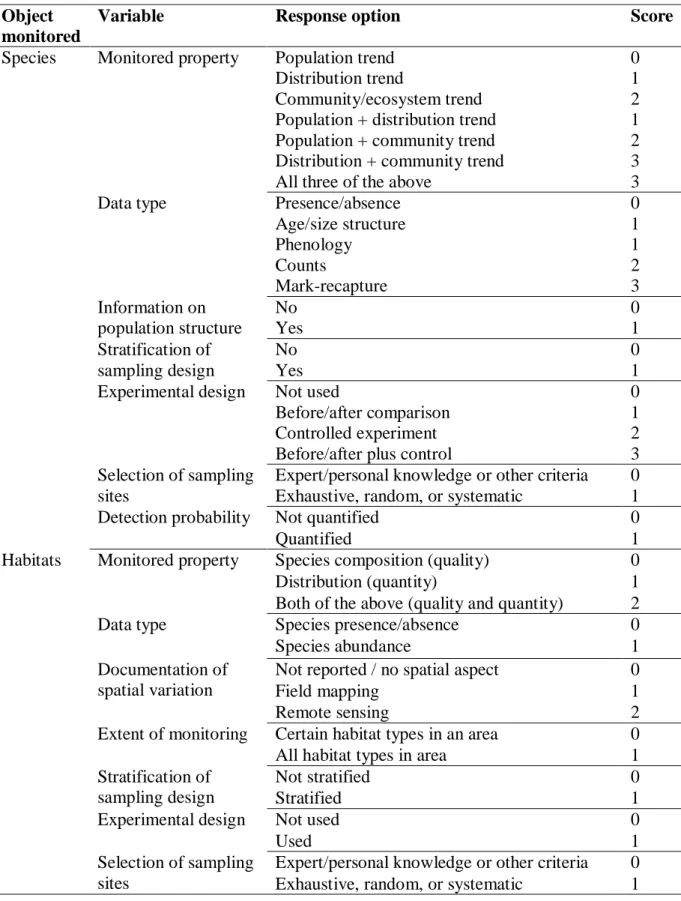
562
Table 1. Scores allocated to different levels of variables describing the sampling design used
563
in species and habitat monitoring schemes in Europe. Please see Supporting Information for
564
justification of score values.
565
Object monitored
Variable Response option Score
Species Monitored property Population trend 0
Distribution trend 1
Community/ecosystem trend 2
Population + distribution trend 1
Population + community trend 2
Distribution + community trend 3
All three of the above 3
Data type Presence/absence 0
Age/size structure 1
Phenology 1
Counts 2
Mark-recapture 3
Information on population structure
No 0
Yes 1
Stratification of sampling design
No 0
Yes 1
Experimental design Not used 0
Before/after comparison 1
Controlled experiment 2
Before/after plus control 3
Selection of sampling sites
Expert/personal knowledge or other criteria 0 Exhaustive, random, or systematic 1
Detection probability Not quantified 0
Quantified 1
Habitats Monitored property Species composition (quality) 0
Distribution (quantity) 1
Both of the above (quality and quantity) 2
Data type Species presence/absence 0
Species abundance 1
Documentation of spatial variation
Not reported / no spatial aspect 0
Field mapping 1
Remote sensing 2
Extent of monitoring Certain habitat types in an area 0
All habitat types in area 1
Stratification of sampling design
Not stratified 0
Stratified 1
Experimental design Not used 0
Used 1
Selection of sampling sites
Expert/personal knowledge or other criteria 0 Exhaustive, random, or systematic 1
566
24
Table 2. Means ± standard deviations (S.D.) of sampling design score (SDS) and the
567
temporal sampling effort index (SEtemp) in species and habitat monitoring schemes; N:
568
number of schemes with metadata.
569
SDS SEtemp
Monitored object Mean S.D. N Mean S.D. N
Taxon group in species monitoring
Lower plants 4.9 1.63 22 3.3 0.77 20
Higher (vascular) plants 4.8 2.14 41 3.4 1.07 39
Arthropods (mainly insects) 5.1 2.00 34 3.6 1.05 27
Butterflies 5.0 1.97 38 4.1 1.26 34
Fish and macroinvertebrates 5.3 1.93 27 3.2 0.99 23
Amphibians and reptiles 5.2 1.83 43 4.0 0.91 40
Birds in general 5.2 1.74 59 4.2 1.15 54
Birds of prey 5.8 2.19 21 4.4 1.00 20
Waterbirds 4.8 1.66 53 4.5 1.03 52
Songbirds 5.4 1.82 27 4.3 0.78 27
Bats 4.1 2.07 23 3.3 0.77 22
Small mammals 4.6 1.91 28 3.7 0.93 27
Large mammals 4.5 1.69 40 3.7 1.03 34
Multiple taxon groups 5.7 1.77 14 3.9 0.79 10
All taxon groups combined 5.0 1.89 470 3.9 1.08 429
EUNIS category in habitat monitoring
A marine only 5.3 1.92 12 3.4 0.16 3
AB marine and coastal 5.6 1.75 11 3.7 1.31 2
B coastal only 6.5 2.83 16 3.0 0.92 10
C wetlands 4.2 2.09 11 3.7 1.20 4
D heaths and fens 5.7 3.01 13 3.3 0.64 10
E grasslands 5.5 2.37 16 3.2 0.62 15
F scrubs 6.8 2.48 6 4.0 0.37 3
G forests 5.2 1.66 41 3.4 1.01 25
H caves 6.5 0.71 2 5.4 − 1
I arable land 5.5 0.71 2 3.7 0.45 2
X habitat complexes 6.0 2.14 8 3.2 0.80 7
All habitat types in an area 5.0 2.35 38 3.3 1.37 22
All EUNIS habitat categories combined 5.4 2.23 176 3.3 0.98 104
570 571 572
25
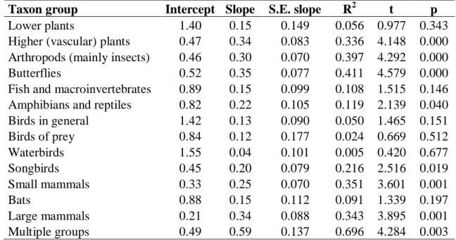
Table 3. Parameters estimated from an ordinary least-squares regression of the number of
573
sampling sites over the area monitored in species monitoring schemes targeting major
574
taxonomic groups
575
Taxon group Intercept Slope S.E. slope R2 t p
Lower plants 1.40 0.15 0.149 0.056 0.977 0.343
Higher (vascular) plants 0.47 0.34 0.083 0.336 4.148 0.000 Arthropods (mainly insects) 0.46 0.30 0.070 0.397 4.292 0.000
Butterflies 0.52 0.35 0.077 0.411 4.579 0.000
Fish and macroinvertebrates 0.89 0.15 0.099 0.108 1.515 0.146 Amphibians and reptiles 0.82 0.22 0.105 0.119 2.139 0.040 Birds in general 1.42 0.13 0.090 0.050 1.465 0.151
Birds of prey 0.84 0.12 0.177 0.024 0.669 0.512
Waterbirds 1.55 0.04 0.101 0.005 0.420 0.677
Songbirds 0.45 0.20 0.079 0.216 2.516 0.019
Small mammals 0.33 0.25 0.070 0.351 3.601 0.001
Bats 0.88 0.15 0.112 0.091 1.339 0.197
Large mammals 0.21 0.34 0.088 0.343 3.895 0.001
Multiple groups 0.49 0.59 0.137 0.696 4.284 0.003
576 577
26
FIGURE LEGENDS
578 579
Figure 1. Sampling design score (SDS) in species monitoring schemes vs. starting period
580
(A), funding source (B), motivation (C) and geographic scope (D). Boxplots show the median
581
(horizontal line), the 25th and 75th percentile (bottom and top of box, respectively),
582
minimum and maximum values (lower and upper whiskers) and outliers (dots).
583
Abbreviations: (B): EU - European Union, nat - national, reg - regional, sci - scientific grant,
584
priv - private source, oth - other; (C) dir - directive, intl - international law, nlaw - national
585
law, sci - scientific interest, mgmt - management/restoration, oth - other reason; (D) EU -
586
European, intl - international, nat - national, reg - regional, loc - local.
587 588
Figure 2. Temporal sampling effort (SEtemp) in species monitoring schemes.
589
(Abbreviations: Fig. 1)
590 591
Figure 3. Spatial sampling effort (SEspatial) in species monitoring schemes. (Abbreviations:
592
Fig. 1)
593 594
Figure 4. Sampling design score (SDS) in habitat monitoring schemes. (Abbreviations: Fig.
595
1)
596 597
Figure 5. Temporal sampling effort (SEtemp) in habitat monitoring schemes. (Abbreviations:
598
Fig. 1)
599 600
Figure 6. Spatial sampling effort (SEspatial) in habitat monitoring schemes. (Abbreviations:
601
Fig. 1)
602 603
27
FIGURES
604 605
Fig. 1
606
607 608
28
Fig. 2
609
610 611
29
Fig. 3
612
613 614
30
Fig. 4
615
616 617
31
Fig. 5
618
619 620
32
Fig. 6
621
622