1
Distribution of niche spaces over different homogeneous river sections at seasonal
1
resolution
2 3
István Gábor Hatvania*, Péter Tanosb, Gábor Várbíróc,d, Miklós Aratóe,f, Sándor Molnárb, Tamás
4
Garamhegyig, József Kovácsg
5
6
aInstitute for Geological and Geochemical Research, Research Center for Astronomy and Earth
7
Sciences, MTA, H-1112 Budapest, Budaörsi út 45, Hungary; hatvaniig@gmail.com
8
bSzent István University, Department of Mathematics and Informatics, H-2100 Gödöllő, Páter
9
Károly utca 1, Hungary; molnar.sandor@gek.szie.hu, tanospeter@gmail.com
10
cMTA Centre for Ecological Research, Danube Research Institute Department of Tisza River
11
Research, H-4026 Debrecen, Bem tér 18/C, Hungary; varbiro.gabor@okologia.mta.hu
12
dMTA Centre for Ecological Research, GINOP Sustainable Ecosystems Group, 3. Klebelsberg
13
Kuno str., H-8237 Tihany, Hungary
14
eEötvös Loránd University, Department of Probability Theory and Statistics, H-1117 Budapest,
15
Pázmány Péter stny. 1/C, Hungary; arato@math.elte.hu
16
fMTA Alfréd Rényi Institute of Mathematics, H-1053 Budapest, Reáltanoda u. 13-15, Hungary;
17
arato@renyi.hu;
18
gEötvös Loránd University, Department of Physical and Applied Geology, H-1117 Budapest,
19
Pázmány Péter stny. 1/C, Hungary; kevesolt@gmail.com, garam999@gmail.com
20
2 21
*Corresponding author address: Institute for Geological and Geochemical Research,
22
Research Center for Astronomy and Earth Sciences, MTA, H-1112 Budapest, Budaörsi út 45,
23
Hungary. Tel.: +36 70 317 97 58; fax: +36 1 31 91738. E-mail: hatvaniig@gmail.com
24
25
Abstract:
26
Planktic algae have an essential role in the food web as primary producers; the
27
determination of the ecological niche space occupied by them is thus essential in strategies aimed
28
at sustaining the biodiversity of surface waters. In the present study, principal component analysis
29
combined with the outlying mean index was applied to 14 water quality time series (1993-2005)
30
derived from three previously determined homogeneous sections of the Hungarian part of the
31
River Tisza. As a result, the seasonal distribution of the ecological n-dimensional hypervolumes
32
was determined for the different river sections. In the first upper section, the seasonal niches
33
overlay each other, and no clear separation could be detected. In the middle- and lower reaches,
34
however, a clear separation between the seasons was observed. The identification of these
35
separate niches of the various seasons as the main indicators/drivers of certain ecological
36
communities (e.g. phytoplankton) proved possible.
37
38
Keywords: combined cluster and discriminant analysis, homogeneous groups, hydrochemical
39
seasons, niche space, principal component analysis
40 41
3
1. Introduction
42
The role of planktic algae as primary producers in the aquatic food webs is well-
43
established; they have a clear and substantial role in shaping the composition of biota of aquatic
44
ecosystems (Wehr and Descy, 1998) with chemical-, physical-, and biological factors defining the
45
structure of phytoplankton communities (Reynolds, 1984; 1996; 2006). These factors may be
46
considered as those determining an n-dimensional hypervolume within which a species can
47
persist, i.e. an ecological niche (Dolédec et al., 2000; Blonder et al., 2014). The precise
48
determination of such niches, and thus their indicators, is essential in phytoplankton ecology, as it
49
demonstrates the environmental position of the community. One of the first steps in defining a
50
niche is the definition of this n-dimensional hypervolume, and this may be achieved using a set of
51
multivariate data analysis techniques, e.g. correspondence analysis (Hill, 1974), canonical
52
correspondence analysis (Pappas and Stoermer, 1997), redundancy analysis (Ter Braak, 1987), or
53
the outlying mean index (Dolédec et al., 2000; Karasiewicz et al., 2017).
54
The concept of ecological niches has attracted great interest with the growing awareness of
55
environmental change, especially in terms of the study of the impacts of niche shifts within a
56
community (Karasiewicz et al., 2017) in aquatic environments (Peterson, 2011). It is generally
57
accepted that water quality sampling units displaying similar behaviors may be expected to
58
support similar communities. So changes in environmental gradients (Dolédec et al., 2000) will
59
therefore indicate, and drive the change in the communities. By exploring the niche spaces in sets
60
of sampling sites rather than unique ones, the number of data assessed can be increased.
61
Therefore, the n-dimensional hypervolume determination of homogeneous groups of sampling
62
sites could enhance the robustness and significance of the obtained ecological models.
63
4
Finding an optimal classification of sampling sites, for e.g. monitoring network
64
optimization, is a common task in the fields of biology, ecology, geology, geography, and related
65
disciplines. However, a classification which is “simply” optimal does not necessarily ensure
66
homogeneity (Kovács et al., 2014). The increasing number of studies setting as their aim the
67
determination of not only similar, but homogeneous groups of sampling sites in lakes (Kovács et
68
al., 2014), rivers (Tanos et al., 2015; Kovács et al., 2015) or subsurface water systems (Kovács et
69
al., 2015) provides an opportunity to explore n-dimensional hypervolumes in subsets of multiple
70
sampling sites in which the members/elements share equal underlying processes (Kovács et al.,
71
2014). The assessment of variables measured in homogeneous groups therefore provides a good
72
opportunity to increase the amount of data obtained from domains with the same environmental
73
conditions (global niche; Karasiewicz et al., 2017).
74
The determination of n-dimensional hypervolumes is frequently performed spatially to
75
assess the degree of phylogenetic relatedness between e.g. various amphibian taxa (Hof, 2010),
76
instream invertebrates (Heino, 2015; Heino and Grönroos, 2014) within a geographical region.
77
The other most frequently considered aspect is seasonal shifts in the niche of taxa (Mérigoux and
78
Dolédec, 2004).
79
The aim of the present study was therefore, to explore how changes in the n-dimensional
80
hypervolumes along the River Tisza (Central Europe’s second largest potamal river), between the
81
river’s homogeneous sub-regions in space and time may indicate changes in the composition of
82
phytoplankton communities. It is expected that the position and breadth of the niche spaces of the
83
seasons will change in space, delineating those seasons. A clear separation would enable the
84
5
development of strategies for sustaining different communities in the different sections of the
85
riverine ecosystems.
86
87
2. Materials and methods
88
The River Tisza gathers the waters of the Carpathian Basin’s Eastern region. It is a highly
89
important ecological corridor (Zsuga et al., 2004), stretching through 5 countries (966 river km,
90
594.5 in Hungary) from its spring in the Eastern Carpathians in the Ukraine to its confluence with
91
the Danube at Titel in Serbia. Its watershed is 157,186 km2 (Lászlóffy, 1982), of which approx.
92
47,000 km2 is located in Hungary. The average annual runoff of the Tisza is 25.4106 m3 (Pécsi,
93
1969). In Hungary, the river’s water quality directly affects the lives of approx. 1.5 m inhabitants.
94
Heading downstream along the river’s Hungarian section, the following tributaries are
95
worth mentioning: the Szamos, Bodrog, Sajó, Zagyva, Kőrös, and Maros rivers (Fig. 1). Based on
96
the runoff of these tributaries, the Szamos might be expected to have the strongest effect on the
97
main flow (at its mouth its average runoff exceeds half of the average runoff of the Tisza; Tanos,
98
2017). Moreover, a considerable “changing effect” is to be expected from the Bodrog, Sajó,
99
Zagyva, Kőrös, and Maros Rivers in relation to the periodic behavior of the river.
100
Besides these tributaries, other, mostly anthropogenic factors, such as water barrage
101
systems (WBS; e.g. Tiszalök WBS, Fig. 1), or lakes (e.g. Kisköre Reservoir; Fig. 1) affect the
102
water quality of river sections (Kentel and Alp, 2013; Moreira and Poole, 1993). Even ice regime
103
changes may occur on rivers due to the installation of WBSs as seen on other Central European
104
rivers (Takács et al., 2013; Takács and Kern, 2015; Takács et al., 2018).
105
6
An artificial lake exists on the river, Kisköre Reservoir (also known as Lake Tisza; length:
106
27 km, mean depth: 1.3 m, total area: 127 km2), constructed in 1973, and planned to function as a
107
part of a future WBS. Nowadays, rather than an “industrial” installation it functions as a much-
108
frequented recreation zone and nature reserve. In addition, non-point source nutrient loads
109
arriving from agricultural areas have to be accounted for as well (Mander and Forsberg, 2000);
110
there are several large cities along the river (e.g. Szeged at T13) which also have an
111
environmental impact on the river’s water quality (Fig.1).
112
The previously mentioned factors (tributaries, WBS etc.), together with the fact that
113
downstream the River Tisza is increasingly becoming a lower section river, have caused the
114
sampling sites of the river (Fig. 1) to form homogeneous groups, characterizing sub-sections with
115
essentially different water quality (Tanos et al., 2015). The uppermost group of homogeneous
116
sampling sites (T3 & T4) represents the transition zone between the hydrologically upper and
117
middle sections of the River Tisza (Várbíró et al., 2007). Here, the water is still transparent, but
118
after the Szamos River, the amount of nutrients increases, dissolved oxygen decreases and the
119
sediment is mainly coarse grained sand. The middle homogeneous group of sampling sites (T7 &
120
T8) is located just upstream of the WBS. The water quality is affected mainly by the damming of
121
the WBS and nutrient input from the Bodrog and Sajó rivers. The lowest group (T12 & T13)
122
mirrors a clearly formed middle-section type of river. It is characterized by a decreased flow
123
velocity and elevated nutrient content brought by the River Kőrös to the main channel (Tanos et
124
al., 2015; Tanos, 2017)..
125 126
7 127
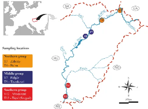
Fig. 1. Hungarian section of the River Tisza and its explored sampling sites. The similar
128
color circles around the codes of the sampling sites indicate that those belong to the same
129
homogeneous group defined in Tanos et al. (2015).
130 131
In the course of the analyses, the time series of 14 water quality variables (Table 1) for the
132
years 1993-2005 from 6 sampling sites (Fig. 1) were examined. The parameters were sampled by
133
various water inspectorates weekly and biweekly. Due to the large area monitored, these samples
134
were not taken on the same day. Thus, after 2005, the sampling frequency was rarefied and the
135
set of parameters changed. The number of data analyzed was ~50,000 in total.
136 137
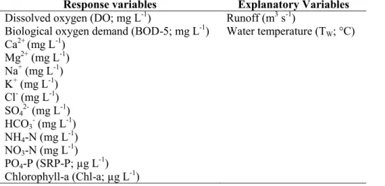
Table 1. Variable groups of response and explanatory water quality variables
138
measured in the Hungarian section of the River Tisza (1993-2005).
139
8 Response variables Explanatory Variables
Dissolved oxygen (DO; mg L-1) Runoff (m3 s-1)
Biological oxygen demand (BOD-5; mg L-1) Water temperature (TW; °C) Ca2+ (mg L-1)
Mg2+ (mg L-1) Na+ (mg L-1) K+ (mg L-1) Cl- (mg L-1) SO42- (mg L-1) HCO3- (mg L-1) NH4-N (mg L-1) NO3-N (mg L-1) PO4-P (SRP-P; µg L-1) Chlorophyll-a (Chl-a; µg L-1) 140
To be able to interpret the results in light of the seasonality of phytoplankton assemblages,
141
phytoplankton composition data was used available for2007-2010. The related investigations
142
were carried out by regional water authorities and research institutions. The original database
143
contained the relative abundance of the species. These species were then sorted into different
144
algal functional groups (codons) according to Reynolds et al. (2002) and Padisák et al. (2009) and
145
their abundance was determined (Table 2) for the homogeneous sections of the River Tisza
146
(Tanos et al., 2015). For details see Fig. 1 and Section 2.1.2.
147
148
Table 2. Phytoplankton codon group’s average relative abundance in the homogeneous
149
river sections (Tanos et al., 2015) of the River Tisza (2007-2010). Abundances > 5 % are
150
highlighted in bold.
151
Codon
group Northern Middle Southern
A 1% 0% 1%
B 23% 9% 13%
C 17% 31% 11%
9
D 21% 27% 17%
E 1% 0% 0%
F 0% 0% 0%
G 0% 0% 0%
H1 1% 0% 16%
J 5% 7% 10%
K 1% 0% 0%
LM 0% 0% 0%
LO 0% 0% 2%
M 0% 0% 0%
P 3% 1% 8%
S1 3% 0% 5%
S2 0% 0% 0%
SN 0% 0% 0%
T 0% 0% 0%
TIB 24% 9% 11%
TIC 0% 1% 0%
TID 0% 0% 1%
U 0% 0% 0%
V 3% 0% 0%
W0 9% 8% 1%
W1 1% 2% 9%
W2 1% 0% 4%
WS 1% 0% 0%
X1 5% 9% 7%
X2 5% 8% 0%
X3 5% 4% 3%
Y 6% 4% 14%
YPh 0% 0% 0%
152
2.1. Methodology
153
2.1.1. Principal component analysis and niche characterization
154
The backbone of the present study was principal component analysis (PCA), a frequently
155
used multidimensional data analysis technique (Tabachnik and Fidell, 1996), mainly applied for
156
dimension reduction. In the present study, the PCs were considered based on their scree plots
157
(Catell, 1966) takin only those into account which had an eigenvalue >1 (Kaiser (1960), thus the
158
10
13 dimensional dataset at hand was reduced to 3 dimensional vectors with uncorrelated
159
coordinates using the first three principal components. It should be noted that in the study the
160
observations’ principal components are referred to as PC scores, while the elements of the
161
eigenvectors of the empirical correlation matrix will be referred to as loadings. These measure the
162
relationship of the coordinates and the PCs with Pearson correlation coefficient. Only those
163
loadings falling outside the ±0.6 interval are considered meaningful.
164
Niche position and niche breadth were determined using the Outlying Mean Index (OMI)
165
analysis (Dolédec et al., 2000). OMI usually measures the marginality of species’ habitat
166
distribution across a given study area (Heino and Soininen, 2006), with the correlation matrix of
167
environmental variables and the occurrence of different species as inputs in the different
168
geographical regions. In the present case, the input correlation matrix was derived from the
169
response water quality variables (Table 1), while in the place of the occurrence of species,
170
hydrochemical seasons are the subject of the niches. In practical terms, this means that the
171
occurrence of the season is the target variable. Thus the niche position, marginality and tolerance
172
of each season and its characteristics are tested along the watercourse.
173 174
2.1.2. Steps in the analysis
175
The homogeneous sections of the Hungarian part of the River Tisza were considered in
176
order to explore the stochastic relationship of its water quality variables and determine its niche
177
space. First, the time series of the response variables (Table 1) of the homogeneous groups of
178
sampling sites (two sites per group, as previously determined by CCDA - Tanos et al., 2015),
179
were taken into account. Briefly, CCDA compares all combinations of hierarchical cluster groups
180
11
to random groupings and suggests the further division of the obtained cluster groups using linear
181
discriminant analysis (Kovács et al., 2014).
182
The time series of the homogeneous groups were then assessed using exploratory principal
183
component analysis (Rogerson, 2001). It is presumed that this will afford an insight into the
184
linear relationship of the water quality variables in the homogeneous groups and lead to a better
185
understanding of the given river sub-section (Tanos et al., 2011). Moreover, by assigning a
186
seasonal (e.g. winter, spring) tag to the data and visualizing the PCA results on bi-plots, the
187
importance of a given response variable in a given season can be determined.
188
As a next step, the obtained PCs were correlated with the explanatory variables’ (Table 1)
189
time series measured in the homogeneous groups themselves, providing information on how
190
water temperature and runoff affect the stochastic relations (background factors).
191
As final step, the n-dimensional hypervolumes (Blonder et al., 2014) were determined for
192
the three homogeneous sections of the River Tisza, taking hydrochemical seasonality (Tanos et
193
al., 2015) into account as well.
194
All computations were performed using R 3.2.3 (R Core Team, 2015), Vegan (Oksanen
195
et al., 2018) and ade4 (Dray et al., 2007) packages and MS Excel 2016.
196 197
3. Results
198
The research was conducted on the homogeneous groups of sampling sites: Northern,
199
Middle, and Southern groups (Fig. 1) previously objectively determined by Tanos et al. (2015)
200
12
using Combined Cluster and Discriminant Analysis (CCDA) (Kovács et al., 2014) on a set of
201
water quality variables similar to that assessed in the present study.
202 203
3.1. General overview
204
In the assessed river sections, the concentration of ions did not vary to a high degree
205
between the homogeneous groups of sampling sites However, DO content and BOD displayed a
206
clear decreasing trend. While Chl-a and runoff indicated a continuous increase in absolute values,
207
SRP slightly decreased in the Middle group.By the time the nutrients (Chl-a and SRP-P) had
208
reached the Southern group, they had increased by ~20 and ~35% respectively in mean
209
concentration compared to the values found in the Northern Group (Table 3).
210
In general, the variability – based on the coefficients of variation (CV; Table 3) - of the
211
observed water quality variables decreased downstream, with e.g. the N forms, BOD displaying a
212
decreasing and then slightly increasing trend downstream. Still, the CVs of the N forms or e.g.
213
BOD in the Southern Group do no exceed those in the Northern Group. It should be noted that
214
the largest decrease in CV was witnessed in the case of Chl-a, where it dropped from ~500% to
215
~110% between the Northern and Southern Groups (Table 3).
216 217
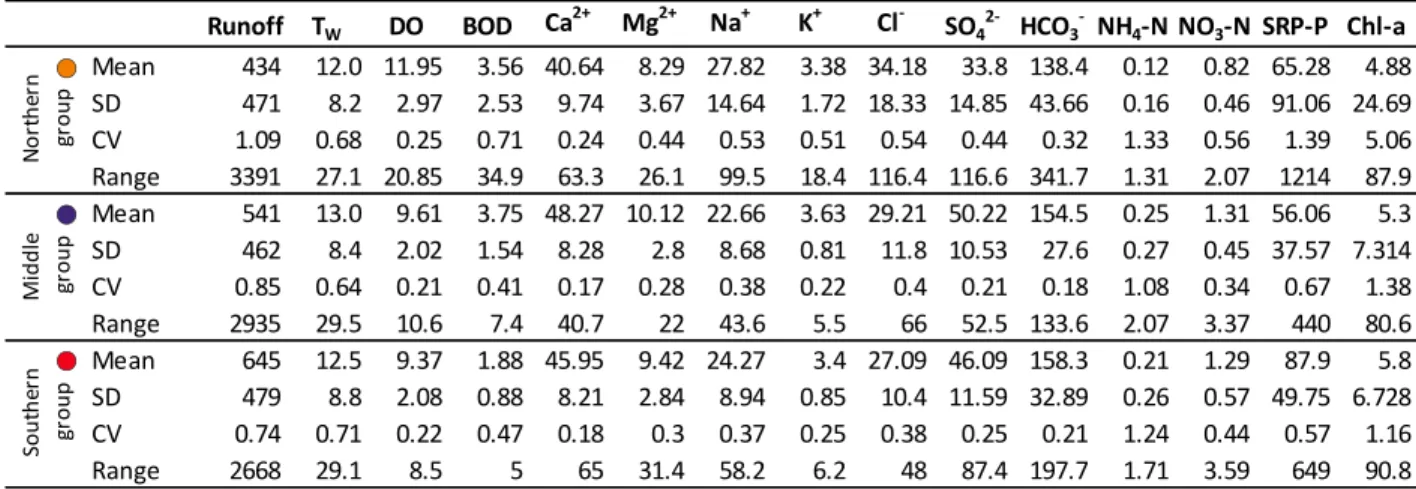
Table 3. Descriptive statistics of water quality variables for each of the homogeneous
218
groups on the River Tisza.
219
13 220
221
3.2. Stochastic relationship of water quality variables in the sub-sections (homogeneous
222
groups) of the River Tisza
223
The cumulative explanatory power of the first three PCs is > 46% in each group, and the
224
percentage of explained variance increases monotonically downstream (Table 4). Between the
225
Northern and Southern groups the explanatory power of PCs almost doubles in the first two PCs,
226
while the third PC explains ~10% of the total variance in every group, regardless of its location.
227
According to the Kaiser-Meyer Olkin criterion, the measure of sampling adequacy (MSA; Kaiser
228
and Rice, 1974) in the Middle and Southern groups is appropriate and very good respectively,
229
while in the Northern group caution has to be taken, since it is <0.5. This is most probably due to
230
the higher variability of water quality in the Northern groups sampling sites compared to the
231
other two groups (Table 3).
232 233
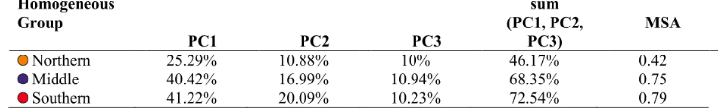
Table 4. Percentage and cumulative percentage of explained variance in the PCs. with
234
Measure of sampling adequacy (MSA) indicated for the correlation matrices of the
235
different groups.
236
Runoff TW DO BOD Ca2+ Mg2+ Na+ K+ Cl- SO42-
HCO3-
NH4-N NO3-N SRP-P Chl-a Mean 434 12.0 11.95 3.56 40.64 8.29 27.82 3.38 34.18 33.8 138.4 0.12 0.82 65.28 4.88 SD 471 8.2 2.97 2.53 9.74 3.67 14.64 1.72 18.33 14.85 43.66 0.16 0.46 91.06 24.69 CV 1.09 0.68 0.25 0.71 0.24 0.44 0.53 0.51 0.54 0.44 0.32 1.33 0.56 1.39 5.06 Range 3391 27.1 20.85 34.9 63.3 26.1 99.5 18.4 116.4 116.6 341.7 1.31 2.07 1214 87.9 Mean 541 13.0 9.61 3.75 48.27 10.12 22.66 3.63 29.21 50.22 154.5 0.25 1.31 56.06 5.3 SD 462 8.4 2.02 1.54 8.28 2.8 8.68 0.81 11.8 10.53 27.6 0.27 0.45 37.57 7.314 CV 0.85 0.64 0.21 0.41 0.17 0.28 0.38 0.22 0.4 0.21 0.18 1.08 0.34 0.67 1.38 Range 2935 29.5 10.6 7.4 40.7 22 43.6 5.5 66 52.5 133.6 2.07 3.37 440 80.6 Mean 645 12.5 9.37 1.88 45.95 9.42 24.27 3.4 27.09 46.09 158.3 0.21 1.29 87.9 5.8 SD 479 8.8 2.08 0.88 8.21 2.84 8.94 0.85 10.4 11.59 32.89 0.26 0.57 49.75 6.728 CV 0.74 0.71 0.22 0.47 0.18 0.3 0.37 0.25 0.38 0.25 0.21 1.24 0.44 0.57 1.16 Range 2668 29.1 8.5 5 65 31.4 58.2 6.2 48 87.4 197.7 1.71 3.59 649 90.8 Northern groupMiddle groupSouthern group
14 Homogeneous
Group
PC1 PC2 PC3
sum (PC1, PC2,
PC3) MSA
Northern 25.29% 10.88% 10% 46.17% 0.42
Middle 40.42% 16.99% 10.94% 68.35% 0.75
Southern 41.22% 20.09% 10.23% 72.54% 0.79
237
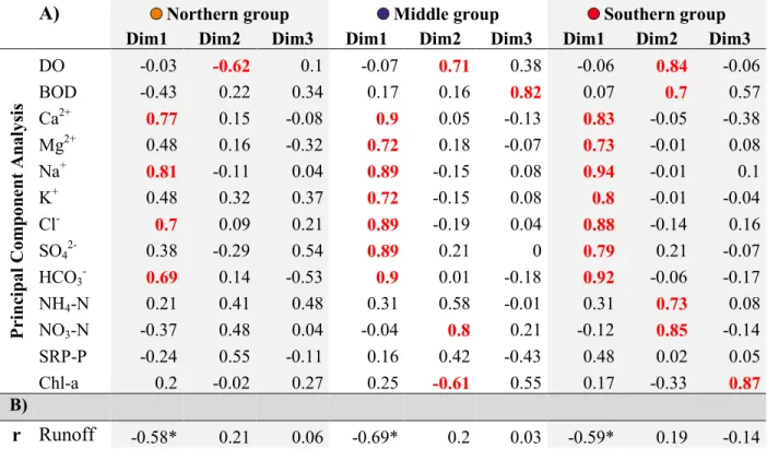
From the perspective of dependent variables, in all of the homogeneous group of sampling
238
sites, in the first PC the ions are the most determining (Table 5a). In the 2nd PC, the degree to
239
which variance is explained is mostly determined by DO; this is true of all three groups, what is
240
more, with an increasing degree of importance downstream (increased loadings in absolute
241
value). Furthermore, downstream of the Northern group, DO changes its sign relative to the ions
242
(Table 5a). In the Northern group, neither nitrate-nitrogen nor Chl-a plays an important role in
243
any of the PCs, unlike in the other two groups downstream. It should be noted that in the Middle
244
group Chl-a has a high loading (-0.61) in the 2nd PC, while in the Southern group this was with
245
the 3rd PC ( loading: 0.87; Table 5a). In the Middle- and Southern groups, BOD also takes on an
246
importance with a PC loading >0.7. Regarding the 3rd PC, in the Northern group, there is no
247
variable which can be considered as a main factor.I In the Middle group’s 3rd PC BOD and, as
248
previously stated, in the Southern group’s 3rd PC, Chl-a becomes the most important factor
249
(Table 5a).
250
With regard to the independent variables, over the whole river section, in every group
251
runoff displays a significant negative correlation only with the first PC (i.e. that which is
252
determined to the greatest extent by ions) (Table 5b). This indicates that when runoff increases,
253
the amount of ions decreases.. The other available explanatory variable, water temperature (Tw),
254
showed a significant linear relationship with only the second PC of the Middle and Southern
255
15
groups (r<-0.8; Table 5b). Since, DO has a positive relationship with the 2nd PC while TW has a
256
negative relationship with it, this reflects the notion that with the increase of TW, the amount of
257
DO decreases in the Middle- and Southern groups. In the case of nitrate-nitrogen a similar
258
relationship is also to be observed in the Middle group, where with the increase of TW, Chl-a is
259
expected to increase as well (Table 5). The conclusion may therefore be drawn that in the
260
Middle- and Southern groups, of the available independent variables, TW plays the most
261
determining role in relation to the biological processes represented by the 2nd PC (Table 5b).
262 263
Table 5. Loadings of the assessed (response) water quality variables in the first three principal 264
components A) and the correlation coefficients of the explanatory variables and the obtained PCs 265
B). Loadings in red are outside the chosen ±0.6 interval (A) and the significant (p<0.05) correlation 266
coefficients (r) are marked with an asterisk (*) in paned (B).
267
A) Northern group Middle group Southern group
Dim1 Dim2 Dim3 Dim1 Dim2 Dim3 Dim1 Dim2 Dim3
Principal Component Analysis
DO -0.03 -0.62 0.1 -0.07 0.71 0.38 -0.06 0.84 -0.06
BOD -0.43 0.22 0.34 0.17 0.16 0.82 0.07 0.7 0.57
Ca2+ 0.77 0.15 -0.08 0.9 0.05 -0.13 0.83 -0.05 -0.38
Mg2+ 0.48 0.16 -0.32 0.72 0.18 -0.07 0.73 -0.01 0.08
Na+ 0.81 -0.11 0.04 0.89 -0.15 0.08 0.94 -0.01 0.1
K+ 0.48 0.32 0.37 0.72 -0.15 0.08 0.8 -0.01 -0.04
Cl- 0.7 0.09 0.21 0.89 -0.19 0.04 0.88 -0.14 0.16
SO42- 0.38 -0.29 0.54 0.89 0.21 0 0.79 0.21 -0.07
HCO3- 0.69 0.14 -0.53 0.9 0.01 -0.18 0.92 -0.06 -0.17
NH4-N 0.21 0.41 0.48 0.31 0.58 -0.01 0.31 0.73 0.08 NO3-N -0.37 0.48 0.04 -0.04 0.8 0.21 -0.12 0.85 -0.14 SRP-P -0.24 0.55 -0.11 0.16 0.42 -0.43 0.48 0.02 0.05
Chl-a 0.2 -0.02 0.27 0.25 -0.61 0.55 0.17 -0.33 0.87
B)
r Runoff -0.58* 0.21 0.06 -0.69* 0.2 0.03 -0.59* 0.19 -0.14
16 TW 0.19 -0.13 -0.08 0.068 -0.82* -0.12 0.11 -0.83* 0.25 268
3.3. Determination of seasonal n-dimensional hypervolume
269
The n-dimensional hypervolumes of the three homogeneous sections of the river (Fig. 1)
270
made it clear that in the Northern group there is just a marginal difference between the positions
271
and breadth of the niches in relation to the seasons, especially in the 1st PC (Fig. 2a). This was
272
reflected in the power of the linear relationship between the variables, as also with the PCs.
273
These, in turn, were relatively evenly distributed between PC1 and PC2 (Fig. 2a left panel). A
274
slight differentiation is to be seen in the niche space of PC2, detemined primarily by dissolved
275
oxygen (Table 5a). In this niche space only spring occupies a slightly marginal position.
276
In the Middle and Southern groups, separation of the niches of the various seasons, is
277
mostly characteristic in PC1, where winter and summer take the furthermost position from one-
278
another. In the 1st PC the ions were the most determining, and in which spring bore a greater
279
similarity to winter, and fall to summer (Fig. 2b). In PC2, only spring separated from the other
280
seasons, which is mostly determined by the nutrients. This however, is less characteristic in PC2
281
of the Southern group. The only substantial difference between the Middle and Southern groups
282
compared to the Northern group was to be observed in the closer position of the overlapping
283
niche spaces of the seasons, rendering winter almost totally separate from the other seasons in
284
PC1 (Fig. 2b,c). In PC2, only spring separated (Fig. 2b,c)
285 286
17 287
18
Fig. 2. Niche position of water quality observations in an n-dimensional hyperspace across
288
the Hungarian section of the River Tisza. Left column: biplots of the first and second PCs,
289
where black dots represent the observations, rings correspond to the 70% confidence
290
ellipses estimated using the mean niche position for each season in the Northern A), Middle
291
B) and Southern C) groups.
292
Right column: one axis presentation of outlying mean index results for the Northern A),
293
Middle B) and Southern C) groups for PCs 1 and 2 (upper and lower sub-panels,
294
respectively). Species distribution arranged according to site scores (black ticks); mean
295
distribution indicated by a black dot.
296
19
4. Discussion
297
4.1. Stochastic relationships and absolute values of water quality parameters
298
The concentration of the ions in the homogeneous groups of the Hungarian section of the
299
River Tisza did not vary to a significant high degree with the increase of runoff downstream
300
(Tanos et al., 2015), and accounted for most of the variance over the whole river section (Table
301
5). This was reflected in the significant negative correlation between runoff and the first PC
302
(Table 5b), in which ions played the most important role (Table 5a). However, along with flow
303
velocity, the amount of dissolved oxygen also decreased downstream (Cox, 2003), while its
304
importance increased. This, in turn, was reflected in its increased loading of DO in the 2nd PC
305
(Table 5a). Interestingly, BOD did not behave as expected; instead of displaying an increase
306
(Cox, 2003; Huang et al., 2010), BOD decreased. This may be the result of a combination of
307
effects. Due to its macrophyte cover (Lukács et al. 2015)the Kisköre Reservoir is capable of
308
retaining compounds that could lead to an elevated BOD in the lower sections of the river. A
309
similar phenomenon is to be observed in wetlands particularly created for such a purpose
310
(Hatvani et al., 2014, 2017). . Additionally, the River Kőrös does not bring an elevated level of
311
inorganic nutrients (-20-30% compared to the River Tisza;Tanos, 2017). In the meanwhile due to
312
the decreased flow velocity the dissolution of oxygen decreases as well; even the elevated levels
313
of Chl-a content (+ ~20%) (Table 3) cannot compensate for the effects of these processes.
314
The decrease in SRP-P concentration in the Middle group may be related to the damming
315
effect of the water barrage system (Tanos, 2017). This slows the water down, causing increased
316
transparency, thus making a limiting factor of the light and temperature conditions for
317
phytoplankton rather than nutrients (Vukovic et al., 2014). This was also reflected in the
318
20
significant (p<0.05) and strong (r<-0.82) relationship between TW and the 2nd PC of the Middle
319
and Southern groups. In addition, it should be noted that with the characteristics of the river
320
increasingly resembling those of a lower section river (sediment deposition, low turbidity, high
321
transparency (Vukovic et al., 2014)), a continuous increase was seen in the absolute values of
322
phytoplankton biomass (Kovács et al., 2017) and in their degree of importance as well (Tables 3
323
&5a).
324
4.2. Ecological covariances taking seasonality into account
325
Describing the habitat pattern of phytoplankton communities is crucial in determining the
326
range of driving environmental variables (or constraints) in space and time (Vannotte et al.,
327
1980). This habitat pattern could then serve as a revitalized niche of the community. There is a
328
clear change in the niche space downstream in terms of both seasons and the parameters driving
329
water quality. This change refers not only to the composition, but also to the position and breadth
330
of the niche spaces (Table 2). The narrower the breadth, the more specific the niche spaces, and
331
this occurred mostly in spring and summer on the River Tisza (Fig. 2).
332
In the Northern group, ions are the most determining factor, while phytoplankton and water
333
temperature have only a marginal role, as along with DO, on account of the higher turbidity and
334
low transparency of this river sub-section (Table 5). Here the river system is driven mainly by the
335
concentration of ions and not nutrients, thus, the system does not “suffer” from the limitation of
336
inorganic nutrients. This results directly in the uncharacteristic separation of any one of the
337
seasons (with the slight exception of spring) from the others in the niche space (Fig. 2a). In fact,
338
this finding is in accordance with the previously-existing knowledge that aquatic systems
339
dominated by planktic- and benthic diatoms (TIB 1codon) are present in all seasons in upstream
340
21
rhithral river sections (Vannotte et al., 1980; Wang et al., 2018; Table 2.). In general, the main
341
factor most probably causing the change in diatom presence is sedimentation, but due to the
342
relatively short residence time upstream, this does not happen either. Downstream, however, the
343
impact of the changes in physical environment becomes more dominant (Bolgovics et al., 2017;
344
Abonyi, 2012). The positive loading of chloride in the first PCs (loading=0.7; Table 5a) indicate
345
that one of the most dominant diatom species is a halophilic centric diatom (codon C), but this
346
characteristic is also true of other planktic diatoms in the River Tisza and other watercourses as
347
well (B-Béres et al., 2017; Table 2.). The greater the distance from the source, the greater the
348
degree to which seasonality became the main driving force in the structuring of river
349
phytoplankton community composition, with lower TIB- codon and higher J and Y codon ratio
350
(Table 2).
351
The Middle- and Southern groups of the River Tisza behave like the lower part of a
352
potamal river and can be compared to a shallow, but disturbed, lake in which the inorganic
353
nutrient input is a highly limiting factor on phytoplankton communities (Abonyi et al., 2012;
354
Wang et al., 2018). This is reflected in the determining role of the N forms (Table 5a) and the
355
mean niche positions of the seasons. This shift in niche also occurs as a functional shift in
356
phytoplankton (Table 2), as is also the case in the Pearl River system (Wang et al. 2018). These
357
observations are consonant with the fact that the primary nutrients (C, N, P,) in rivers are
358
generally non-limiting factors in phytoplankton biomass (Minaudo et al., 2015). In the case of the
359
River Tisza, this finds reflection in the non-determining role of primary nutrients in relation to
360
the determined niche spaces of the river sections. With regard to seasons, both summer and
361
winter separate in the first PC, while in the second PC, where N forms are dominant, this does not
362
happen. In PC2spring separates from the other seasons (Fig. 2). In similar settings, it has been
363
22
documented (Salmaso, 2003) that in general three types of the phytoplankton occur in a river.
364
The first group includes large late winter/spring tychoplanktic diatoms (Varbiro et al. 2007),
365
which develop in periods of high water turbulence and strong physical control, with high nutrient
366
concentrations. This is clearly mirrored by the large TIB codon abundance in the northern part of
367
the river. These diatoms, however are able to occupy the separate spring niche space determined
368
in PC2 of the Middle- and Southern groups, where the quantity of nutrients and runoff is higher
369
(both N and P increased), concentration of DO is lower than in the North (Table 3).
370
The second group of phytoplankton characterized by codons B, C and D is tolerant to
371
grazing and sinking in stratified, stable conditions, and also of the nutrient-deficient conditions
372
characteristic of the lower reaches of the river. Moreover, since these have different types of
373
nutrient substrates, they are able to tolerate nutrient deficiency, even if this is not their preferred
374
environment.
375
A third group of species (e.g. coenobial chlorococcoid green algae) develop in
376
environmental conditions falling between those preferred by the two preceding types, and are
377
mostly characteristic of the summer season (Salmaso, 2003).
378
Therefore, due to the abrupt spring/early summer change decreasing the degree of
379
physical disturbance, mirrored in the relationship between the time series of the water quality
380
parameters and the PCs (Table 5) and the seasonal separation of the niche spaces (Fig. 2), as
381
summer progresses, the stabilization of environmental factors offers a window to a new group of
382
species. However, in late summer/fall, thanks to increasing rainfall and falling temperature,
383
species characterizing the winter/spring season reenter the community in accordance with typical
384
plankton dynamics.
385
23 386
4. Conclusions
387
By conducting stochastic analyses of the three homogeneous river sections of the
388
Hungarian part of the River Tisza (consisting of multiple sampling sites), it proved possible to
389
look at an increased number of observations, thus enhancing the effectiveness of the predictive
390
models and the robustness of the results.
391
The principal component- and outlying mean index analyses conducted on these datasets
392
indicated that (i) in the upper section of the river, the separation of the ecological niche spaces is
393
not characteristic, while (ii) downstream a seasonal separation of the n-dimensional
394
hypervolumes is to be observed, and (iii) the downstream change in the composition of the
395
driving parameters of water quality (e.g. increased influence of ions and organic components)
396
was responsible for the differentiation of the phytoplankton communities in their reaction to the
397
niche separation.
398
The study provides an example on how the combination of state-of-the-art multivariate
399
statistical methods is able to (i) increase data density without information loss, thus (ii) enhance
400
the robustness of the models and (iii) effectively determine hydrochemical seasons and (iv)
401
indicate both the background factors and also the ecological niches of a riverine ecosystem.
402 403
Acknowledgements
404
We the authors would like to thank Paul Thatcher for his work on our English version. We
405
would also like to give thanks for the support of the MTA “Lendület” program (LP2012-27/2012)
406
24
and the János Bolyai Research Scholarship of the Hungarian Academy of Sciences, the
407
Hungarian Ministry of Human Capacities (NTP-NFTÖ- 17), the Szent István University
408
(FIEK_16-1-2016-0008; EFOP 3.4.3-16-2016-00012). This is contribution No. XX of 2ka
409
Palæoclimate Research Group.
410 411
References
412
Abonyi, A., Leitão, M., Lançon, A.M., Padisák, J., 2012. Phytoplankton functional groups as
413
indicators of human impacts along the River Loire (France). Hydrobiologia, 698(1), 233–
414
249, 10.1007/s10750-012-1130-0.
415
B-Béres, V., Török, P., Kókai, Z., Lukács, Á., Enikő, T., Tóthmérész, B., Bácsi, I., 2017.
416
Ecological background of diatom functional groups: Comparability of classification
417
systems. Ecological Indicators, 82, 183-188.
418
Blonder, B., Lamanna, C., Violle, C. and Enquist, B. J., 2014. The n-dimensional hypervolume.
419
Global Ecology and Biogeography, 23, 595–609.10.1111/geb.12146
420
Bolgovics, Á., Várbíró, G., Ács, É., Trábert, Z., Kiss, K. T., Pozderka, V., Görgényi, J., Boda, P.,
421
Lukács, B-A., Nagy-László, Zs., Abonyi, A., Borics, G., 2017. Phytoplankton of rhithral
422
rivers: Its origin, diversity and possible use for quality-assessment. Ecological Indicators,
423
81, 587-596, 10.1016/j.ecolind.2017.04.052.
424
Cattell, R.B., 1966. The scree test for the number of factors. Multivar Behav Res 1:245–27.
425
Cox, B. A., 2003. A review of dissolved oxygen modelling techniques for lowland rivers. Science
426
of The Total Environment, 314-316, 303-334, 10.1016/S0048-9697(03)00062-7
427
25
Dolédec, S., Chessel, D., Gimaret-Carpentier, C., 2000. Niche separation in community analysis:
428
a new method. Ecology, 81(10), 2914-2927, 10.1890/0012-
429
9658(2000)081[2914:NSICAA]2.0.CO;2
430
Dray, S., Dufour, AB., Chessel, D., 2007. The ade4 package-II: Two-table and K-table methods.
431
R News. 7(2), 47-52.
432
Hatvani, I.G., Clement, A., Kovács, J., Székely Kovács, I., Korponai, J., 2014. Assessing water-
433
quality data: The relationship between the water quality amelioration of Lake Balaton and
434
the construction of its mitigation wetland. Journal of Great Lakes Research, 40(1), 115-125,
435
10.1016/j.jglr.2013.12.010.
436
Hatvani, I.G., Clement, A., Korponai, J., Kern, Z., Kovács, J., 2017. Periodic signals of climatic
437
variables and water quality in a river – eutrophic pond – wetland cascade ecosystem tracked
438
by wavelet coherence analysis. Ecological Indicators, 83, 21-31,
439
10.1016/j.ecolind.2017.07.018.
440
Heino, J., 2015. Deconstructing occupancy frequency distributions in stream insects: effects of
441
body size and niche characteristics in different geographical regions. Ecological
442
Entomology, 40(5), 491-499, 10.1111/een.12214
443
Heino, J., & Grönroos, M., 2014. Untangling the relationships among regional occupancy,
444
species traits, and niche characteristics in stream invertebrates. Ecology and Evolution,
445
4(10), 1931-1942, 10.1002/ece3.1076
446
Heino, J., & Soininen, J., 2006. Regional occupancy in unicellular eukaryotes: a reflection of
447
niche breadth, habitat availability or size‐ related dispersal capacity? Freshwater Biology,
448
51(4), 672-685, 10.1111/j.1365-2427.2006.01520.x
449
26
Hill, MO., 1974. Correspondence Analysis: A Neglected Multivariate Method. Journal of the
450
Royal Statistical Society, 23(3), 340-354, http://www.jstor.org/stable/2347127
451
Huang, F., Wang, X., Lou, L., Zhou, Z., Wu, J., 2010. Spatial variation and source apportionment
452
of water pollution in Qiantang River (China) using statistical techniques. Water research,
453
44(5), 1562-1572.
454
Karasiewicz, S., Dolédec, S., Lefebvre, S., 2017. Within outlying mean indexes: refining the
455
OMI analysis for the realized niche decomposition. PeerJ Preprints 5:e2810v1
456
https://doi.org/10.7717/peerj.3364
457
Kaiser, H.F., 1960. The Application of Electronic Computers to Factor Analysis. Educational and
458
Psychological Measurement, 20, 141-151.
459
Kaiser, H.F. and Rice., J., 1974. Little jiffy, mark iv. Educational and Psychological
460
Measurement, 34(1),111–117.
461
Kentel, E., Alp, E., 2013. Hydropower in Turkey: Economical, social and environmental aspects
462
and legal challenges. Environmental Science & Policy, 31, 34-43,
463
10.1016/j.envsci.2013.02.008.
464
Kovács, J., Kovács, S., Hatvani, I.G., Magyar, N., Tanos, P., Korponai, J., Blaschke, A.P., 2015.
465
Spatial Optimization of Monitoring Networkson the Examples of a River, a Lake-Wetland
466
System and a Sub-Surface Water System. Water Resources Management, 29, 5275-5294,
467
10.1007/s11269-015-1117-5.
468
Kovács, J., Kovács, S., Magyara, N., Tanos, P., Hatvania, IG., Anda, A., 2014.Classification into
469
homogeneous groups using combined cluster and discriminant analysis. Environmental
470
Modelling & Software, 57, 52-59, 10.1016/j.envsoft.2014.01.010
471
27
Lászlóffy, W., 1982. Works on the River Tisza and water management on the Tisza’s water
472
system (in hungarian: A Tisza, vízi munkálatok és vízgazdálkodás a tiszai vízrendszerben).
473
Akadémiai Kiadó, Budapest. 1982.
474
Liu, X., Zhang, Y., Shi, K., Lin, J., Zhou, Y., Qin, B., 2016. Determining critical light and
475
hydrologic conditions for macrophyte presence in a large shallow lake: the ratio of euphotic
476
depth to water depth. Ecological Indicators, 71, 317-326.
477
Lukács, BA., Tóthmérész, B., Borics, G., Várbíró, G., Juhász, P., Kiss, B., Müller, Z., G-Tóth, L.,
478
Erős, T., 2015. Macrophyte diversity of lakes in the Pannon Ecoregion (Hungary).
479
Limnologica-Ecology and Management of Inland Waters, 53, 74-83,
480
10.1016/j.limno.2015.06.002.
481
Mander, Ü., Forsberg, C., 2000. Nonpoint pollution in agricultural watersheds of endangered
482
coastal seas. Ecological Engineering, 14, 317-324, 10.1016/S0925-8574(99)00058-0.
483
Mérigoux, S., Dolédec, S., 2004. Hydraulic requirements of stream communities: a case study on
484
invertebrates. Freshwater Biology, 49(5), 600-613, 10.1111/j.1365-2427.2004.01214.x
485
Minaudo, C., Meybeck, M., Moatar, F., Gassama, N., Curie, F., 2015. Eutrophication mitigation
486
in rivers: 30 years of trends in spatial and seasonal patterns of biogeochemistry of the Loire
487
River (1980–2012). Biogeosciences, 12(8), 2549-2563.
488
Moreira, J.R., Poole, A.D., 1993. Hydropower and its constraints. in: Johansson, T.B., Kelly, H.,
489
Reddy, A.K.N., Williams, R.H. (Eds.), Renewable Energy: Sources for Fuels and
490
Electricity. Island Press, Washington, pp. 73-119.
491
Oksanen, J., Blanchet, FG., Friendly, M., Kindt, R., Legendre, P., McGlinn, D., Minchin, PR.,
492
O'Hara, RB., Simpson, GL., Solymos, P., Stevens, MHH., Szoecs, E., Wagner, H., 2018:
493
28
vegan: Community Ecology Package, CRAN, https://cran.r-
494
project.org/web/packages/vegan/index.html
495
Padisák, J., Crossetti, L.O., & Naselli-Flores, L., 2009. Use and misuse in the application of the
496
phytoplankton functional classification: a critical review with updates. Hydrobiologia,
497
621(1), 1-19.
498
Pappas, JL., Stoermer, EF., 1997. Multivariate measure of niche overlap using canonical
499
correspondence analysis.Ecoscience, 4(2), 240-245,
500
Pécsi M., 1969. Great Plane of the Tisza (in Hungarian). Akadémiai Kiadó, p 382, Budapest.
501
Peterson, A. T., 2011. Ecological niche conservatism: a time-structured review of evidence.
502
Journal of Biogeography, 38: 817–827, 10.1111/j.1365-2699.2010.02456.x
503
R Core Team, 2015. R: A Language and Environment for Statistical Computing. R Foundation
504
for Statistical Computing, Vienna, Austria.
505
Reynolds, C. S. & Descy, J-P., 1996. The production, biomass and structure of phytoplankton in
506
large rivers. Arch. Hydrobiol. 113(Suppl.):161–87.
507
Reynolds, C. S., 2006. The Ecology of Phytoplankton. Cambridge University Press, Cambridge:
508
535.
509
Reynolds, C.S., 1984. Phytoplankton periodicity: the interactions of form, function and
510
environmental variability. Freshwater Biology, 14, 111–142,10.1111/j.1365-
511
2427.1984.tb00027.x.
512
Reynolds, S. Huszar, V., Kruk, C., Naselli-Flores, L., Melo, S., 2002. Towards functional
513
classification of the freshwater phytoplankton. - J. Plankton Res. 24, 417- 428.
514
Rogerson, P.A., 2001. Statistical Methods for Geography. SAGE Publications, London.
515