hjic.mk.uni-pannon.hu DOI: 10.33927/hjic-2020-15
BROWNIAN DYNAMICS SIMULATION OF CHAIN FORMATION IN ELEC- TRORHEOLOGICAL FLUIDS
DÁVIDFERTIG*1, DEZS ˝O BODA1,ANDISTVÁNSZALAI2,3
1Department of Physical Chemistry, University of Pannonia, Egyetem u. 10, Veszprém, 8200, HUNGARY
2Institute of Physics and Mechatronics, University of Pannonia, Egyetem u. 10, Veszprém, 8200, HUNGARY
3Institute of Mechatronics Engineering and Research, University of Pannonia, Gasparich Márk u. 18/A, Zalaegerszeg, 8900, HUNGARY
Brownian dynamics (BD) simulations based on a novel Langevin integrator algorithm are used to simulate the dynamics of chain formation in electrorheological (ER) fluids that are non-conducting solid particles suspended in a liquid that has a dielectric constant different from that of the ER particles. An external electric field induces polarization charge distributions on the spheres’ surfaces that can be modeled as point dipoles in the centers of the spheres. The interaction of these aligned dipoles leads to formation of chains and other aggregates in the ER fluid. In this work, we introduce our methodology and report results for various quantities characterizing the structure of the ER system as obtained with BD simulations. These quantities include the potential energy, diffusion constant, average chain length, chain length distributions, and pair correlation functions. Their behavior as a function of time is presented as the electric field is switched on. The properties of the ER fluid change considerably making this system a potential basic material of many applications.
Keywords: electrorheological fluids, chain formation, Brownian dynamics
1. Introduction
Electrorheological (ER) fluids are [1] suspensions of fine non-conducting solid particles in an electrically insulat- ing liquid. If the particles, imagined as closely spherical, have a dielectric constant that is different from that of the solvent, the arising dielectric boundaries respond to an applied electric field. This dielectric response is the po- larization of the spheres resulting in a polarization charge distribution whose dominant component in the multipole expansion is the dipole moment.
The interactions of these dipoles then lead to a struc- tural change in the ER fluid known as the ER response.
This structural change is basically a formation of chains and other forms of clusters as the polarized spheres are linked together into head-to-tail positions. This structural phase transition is reversible and relatively fast.
This structural change results in a dramatic change in the physical properties of the ER fluid of which the most important is viscosity. This externally controllable, fast and reversible change in viscosity makes ER fluids a kind of a smart material, a central component of devices, such as brakes, clutches, dampers, and valves [2,3]. Such devices have crucial importance in the industry of various fields.
*Correspondence:fertig.david92@gmail.com
The continuously shrinking size of devices resulted in the development of nanotechnology. Understanding the molecular mechanisms behind the workings of nanode- vices is especially important because better understand- ing of microscopic mechanisms can lead to novel designs.
ER devices are also based on microscopic mecha- nisms leading to an emergent macroscopic pattern. No wonder that many modeling studies [4–22] aimed at in- vestigating the microscopic processes behind chain for- mation and corresponding changes in measurable physi- cal properties.
The properties of the ER fluid in the absence of an ap- plied electric field have been investigated by Heyes and Melrose [23]. This means the investigation of the core potential that is either the Lennard-Jones (LJ) fluid or its cut-and-shifted version that is a purely repulsive poten- tial. It has been demonstrated that the repulsive version reproduces experimental behavior better [4].
Cluster formation has been investigated via cluster size distribution [4,9,11,12,20,22], order parameters [12–15,19], mean square displacement and diffusion con- stant [4,6,12], pair distribution functions [6,12], and relaxation times [5,11,12,21]. In particular, Cao et al.
[21] identified relaxation times corresponding to various subprocesses such as initial aggregation, chain formation, and column formation. Identifying these subprocesses is
E
0p
ε
inε
out++ + + + -
- -
- -
σ
Figure 1:Sketch of an ER particle in an external electric field,E0. The dielectric constant inside the sphere isin, while outside the sphere isout. The surface charge dis- tribution,σ(r), induced on the dielectric boundary (Eq. 1) can be approximated by a point dipole,p, in the center of the sphere (Eq. 2).
also our long-term goal. It is also our intention to sim- ulate the ER system in the presence of shear as several authors did [5,6,10,15,21]. These authors investigated shear stress, various terms of viscosity, oscillatory strain, and dependence on strain rate.
In this paper, we do not apply stress, because our main interest is to study the dynamics of the formation of chains with a newly developed simulation package based on a novel Langevin integrator [24–26] as opposed to most studies from the 1990s that used the overdamped limit. We intend to test the program on the ER fluid in the absence and presence of an applied electric field and to follow the dynamics of chain formation when the field is switched on. We characterize this dynamics by plotting energy, mean square displacement, diffusion constant, av- erage chain length, chain length distributions, and radial distribution functions as functions of time.
We use reduced units in this study (seeSection 4) that are closely related to various parameters used in the liter- ature. These parameters characterize the relations of vari- ous effects in the ER fluid. These effects are the polariza- tion (dipole-dipole), thermal, and viscous forces.
The relation of the polarization and thermal forces is often denoted byλand it practically corresponds to the square of the reduced dipole moment used in this study.
It expresses the relation of the ordering effect of electro- static forces and the disordering effect of thermal motion.
The relation of the viscous force to the electrostatic force is called the Mason number (Ma). Many authors plot the characteristic physical quantities as functions of the Ma- son number [5,10,15]. The relation of the viscous and the electrostatic forces is called the Péclet number.
.
2. Model: the polarizable dielectric sphere We model the ER fluid as dielectric spheres of dielectric constantin inside the sphere immersed in a fluid of di- electric constantout(Fig. 1). The radius of the spheres is R, while their diameter isd= 2R. When a constant elec- tric field,E0is applied to this system (in thezdirection), the dielectric boundary on the sphere’s surface becomes
0 π/8 π/4 3π/8 π/2
θ -0.004
-0.002 0 0.002
Intermolecular potential
Permanent dipoles Polarizable dipoles Surface charge
E0 E0
E0 θ
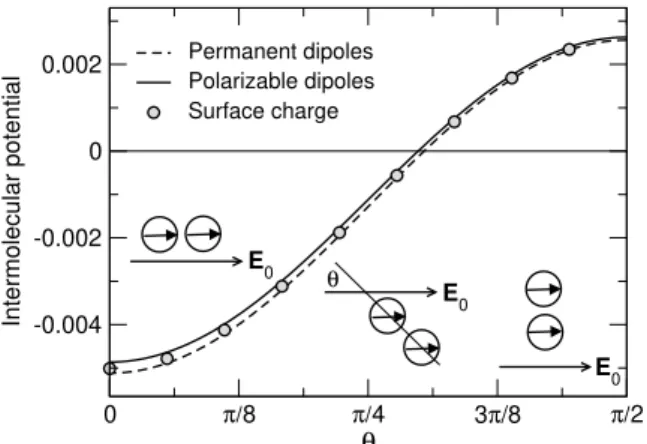
Figure 2: Interaction potential (arbitrary unit) between two dipoles atr= 1.25ddistance from each other at dif- ferent mutual positions characterized by angle θ that is the angle betweenE0andrij. The potential is computed from the interaction of the charge distributions inEq. 1 using the ICC method (symbols), from the interactions of the permanent point dipoles induced only byE0 (Eq. 2) (dashed line), and from the interaction of the polarizable dipoles when the sphere can be polarized by the electric field of other dipoles too (solid line).
polarized. The polarization charge density is σ(θ) = 30
in−out in+ 2out
E0cosθ, (1) whereE0 = |E0|,θ is the angle between the point of on the surface and the z-axis, and 0 is the permittivity of vacuum. As it was discussed in our previous publica- tion [30], the effect of this surface charge distribution can be approximated with an ideal point dipole placed in the center of the sphere computed as [31]
p= 4π0
in−out in+ 2out
R3E0. (2) In that paper, we showed that the point dipole model is a good approximation to the exact solution obtained from the polarization charge using the Induced Charge Compu- tation method [32]. The agreement is better if the spheres are assumed to be polarizable by the electric fields of all the other particles, but even if it is assumed that an ER particle is polarized only by E0, the agreement is rea- sonable (Fig 2). The latter assumption means that the ER particles carry only the permanent dipoles ofEq. 2that always point into thez-direction.
We further assume that the characteristic time of the rearrangement of the surface charge as the particles move is much smaller than the characteristic time of the rota- tion of the particles. This means that thepdipole always points into thezdirection even if the sphere rotates, be- cause the induced charges (that chiefly correspond to po- larization of solvent molecules around the sphere) always have enough time to rearrange themselves according to the applied field,E0.
The potential produced by a dipolepj (that is atrj)
at the positionriof another dipolepiis Φj(ri) = 1
4π0
pj·rij
rij3 , (3) whererij =ri−rjandrij=|rij|. The electric field is
Ej(ri) = 1 4π0
3nij(nij·pj)−pj
r3ij , (4) wherenij = rij/rij. The interaction potential between the two dipoles is
uDDij (rij,pi,pj) =−pi·Ej(ri) =
=− 1 4π0
3(nij·pi)(nij·pj)−pi·pj
r3ij , (5)
while the force exerted on dipolepiby dipolepjis fijDD(rij,pi,pj) =−(pi· ∇i)Ej(ri) =
= 1 4π0
1
rij4 {3 [pi(nij·pj) +pj(nij·pi)+
+ nij(pi·pj)]−15nij(nij·pi)(nij·pj)}. (6) Note that the forms of these equations are simplified when all the dipoles of magnitude pare aligned in the zdirection:
uDDij (rij, θ) =− p2 4π0
3 cos2θ−1
r3ij , (7) and
fDD(rij, θ) = 3p2 4π0
(2 cosθ)k+ (1−5 cos2θ)nij
rij4 ,
(8) wherekis the unit vector in the direction of thez-axis andθ is the angle between k and nij. There is also a torque acting on the dipole, but because the characteris- tic time of polarization charge formation is much smaller than the characteristic time of the rotation of the sphere, the rearrangement of surface charges is considered in- stantaneous without inertia. The torque, therefore, has been neglected.
The full interaction potential between two ER parti- cles consists of this dipole-dipole (DD) term and a short- range core potential that defines the finite size of the par- ticles:
uij=uDDij +uWCAij . (9) For the core potential, we use the cut & shifted LJ poten- tial also known as the Weeks-Chandler-Anderson (WCA) potential that is
uWCAij (rij) =
uLJij(rij) +uLJij(rc) if rij< rc
0 if rij> rc
, (10) where
uLJij(rij) = 4εLJ
" d rij
12
− d
rij
6#
(11)
is the LJ potential. The WCA force is fijWCA(rij) =
fijLJ(rij) if rij< rc 0 if rij> rc
, (12) where
fijLJ(rij) = 24εLJ
"
2 d
rij
12
− d
rij
6# rij
r2ij (13) is the LJ force. In these equations the cutoff distance is rc = 21/6dthat is at the minimum of the LJ potential, so this potential is a smooth repulsive core potential used widely in dynamical simulations of large spherical parti- cles.
3. Method: Brownian Dynamics simulation When it comes to simulating the trajectories of particles in the phase space interacting with each other via a sys- tematic force,fij (like those given inEqs. 6and12), we use Newton’s equation of motion in an MD simulation.
In this case, the particles move in vacuum and the only forces that we take into account are those exerted by the particles themselves (plus, possibly, external forces).
When it comes to simulating the trajectories of parti- cles immersed in a solvent, we use Langevin’s equations of motion [33]
mdvi(t)
dt =Fi(ri(t))−mγvi(t) +Ri(t), (14) whereri,vi,m, andγare the position, the velocity, the mass, and the friction coefficient of particle i, respec- tively. The mass and the friction coefficient are assumed to be the same for every particle, but, in general, they can depend oni.
The force has three components. In addition to the systematic force, Fi(ri(t)) = P
j6=ifij, there are the frictional force,−mγvi(t), and the random force,Ri(t).
The former describes friction, while the latter describes random collisions with surrounding solvent molecules.
The two additional forces represent the interactions with the heat bath and are coupled through the friction coefficient:
hR(t)i= 0 (15) hR(t)·R(t0)i= 2kT mγδ(t−t0) (16) This is also known as the fluctuation–dissipation theo- rem.
The Langevin equation is a stochastic differential equation that is solved numerically and, therefore, ap- proximately. Several algorithms exist in the literature for its integration [34–37].
Here, we employ the simple and effective algorithm of Grønbech-Jensen and Farago (GJF). The original ver- sion [24] had a Verlet-type formalism. Recent modifica- tions by Farago (GJF-F) [25] and Grønbech Jensen and
Table 1:Reduced quantities
Quantity Symbol Unit quantity Reduced quantity
Time t t0=d
rm
kT t∗= t
d rkT
m
Distance r r0=d r∗= r
d
Density ρ ρ0= 1
d3 ρ∗=ρd3
Velocity v v0= d
t0
= rkT
m v∗=v rm
kT
Energy u u0=kT u∗= u
kT
Force F F0=kT
d F∗= F d
kT
Dipole moment p p0=√
4π0kT d3 p∗= p
√4π0kT d3
Friction coefficient γ γ0= 1 t0
=1 d
rkT
m γ∗=γt0=γd rm
kT. Grønbech-Jensen (GJF-2GJ) [26] have a leap-frog for-
malism using velocities in the half time steps. These mod- ifications have the advantage that they accurately sample both kinetic and configurational properties even for large time steps within the stability limit. The authors demon- strated the efficiency of their algorithms for systems un- der linear and harmonic potentials. We use the GJF-2GJ version in this work that reads as
vn+12 =avn−12 +
√b∆t m fn+
√b
2m Rn−Rn+1 (17) rn+1=rn+√
bvn+12∆t, (18) wherern=r(tn)is any position coordinate of any parti- cle,vn=v(tn)is any velocity coordinate of any particle,
a=1−γ∆t/2
1 +γ∆t/2, (19)
b= 1
1 +γ∆t/2, (20)
∆tis the time step,tn+1
2 =tn+∆t2 , andtn−1
2 =tn−∆t2 . The discrete time noise
Rn+1= Z tn+1
tn
R(t0)dt0 (21) is a random Gaussian number with properties
hRni= 0 (22) and
hRmRni= 2kT γm∆tδmn (23) withδmnbeing the Kronecker-delta.
4. Scaling and reduced units
Competing effects exist in an ER system. The DD inter- actions have an ordering effect. The head-to-tail position, in which the dipoles are aligned along nij (θ = 0) at contact (rij=d), has a minimum energy with the value
u0=− 1 4π0
2p2
d3 . (24)
The magnitude of the force in this position is f0= 3p2
4π0d4. (25) The Brownian motion has a disordering effect that ex- presses the coupling to a thermostat of temperatureTand friction with the surrounding solvent with viscosityη. It is usual to characterize the disordering effect of the ther- mal motion energetically by kT. It is also usual to use reduced units in calculations. In reduced units our quanti- ties are expressed as dimensionless numbers obtained by dividing a quantity in a physical unit by a unit quantity in the same unit,t∗ =t/t0, for example. Reduced quanti- ties are useful not only because their values are close to 1, so it is easier to work with them, but also because they express relations between quantities in the numerator and the denominator, a kind of scaling [5].
There are different ways of defining reduced units. We use the convention of building the unit quantities from the mass,m, the particle diameter,d, andkT. Thus, the reduced units collected inTable 1can be defined.
When we perform simulations in reduced units, these quantities can be chosen freely to see how the system be- haves at the different combinations of the reduced param- eters. How the reduced parameters are related to real-life physical parameters can be computed independently (see Section 5).
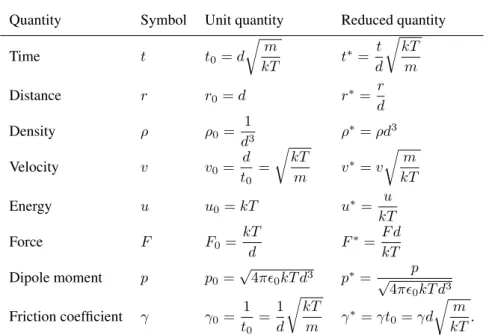
Table 2:Experimental parameters [38,39].
in 4
out 2.7
η(Pa s) 0.5 E0(V/m) 106
T(K) 300
ρout(kg/m3) 2650
The reduced quantities collected inTable 1are deter- mined by the real physical parameters of the system: the temperature,T, the mass density of the material of the ER particle,ρin, the diameter of the ER particle,d, the dielectric constant of the ER particle,in, the dielectric constant of the solvent,out, the viscosity of the solvent, η, and the strength of the applied electric field,E0. For a specific ER fluid, these variables are tabulated inTa- ble 2. This specific example is used because one of the coauthors (I.SZ.) published experimental results for this system [38,39]. A wide variety of ER fluids exists, how- ever.
The mass of a particle is computed asm=ρinπd3/6, so it scales withd3. The dipole moment of a particle is given byEq. 2that shows thatpscales withd3.
An important parameter is the ratio of the dipolar energy and the thermal energy that is expressed by the square of the reduced dipole moment:
(p∗)2= π0E02 4kT
in−out
in+ 2out
2
d3=Kd3 (26) that scales with d3. If p∗ is large, the dipolar interac- tions are strong enough to induce chain formation. Ifp∗is too large, the chains freeze, and the ER particles solidify (note that the fluid itself does not solidify). Ifp∗is small, thermal motion prevents chain formation and/or breaks the chains.
The friction coefficient can be computed from Stokes’
law as
γ= 3πηd m =18η
ρin
d−2. (27)
so it scales with d−2. The value of γ∗ describes the strength of the coupling with the solvent and it scales with d1/2. Ifγ∗is large, friction and the disordering effect of the random force are strong. The diffusivity of the parti- cles in the fluid, therefore, will be smaller. The diffusion constant in the high coupling limit can be expressed by Einstein’s relation:
D= kT
mγ, (28)
or, in reduced units,D∗= 1/γ∗. Ifγ∗→0, the frictional and the random forces vanish, and the Langevin equa- tion goes into the Newton equation. The particles move in vacuum without a thermostat; this practically corre- sponds to an MD simulation in the microcanonical en- semble. Ifγ∗ is small, we talk about an MD simulation with a Langevin thermostat.
In the case of the ER fluids, we are in the regime of largeγ∗. As we will see,γ∗is in the order of104−106. In this case, our concern is how to make the simulation efficient in order to collect enough information about the dynamics of the system in a reasonable amount of com- puter time.
The parameter with which we can tune the speed of sampling is the time step, ∆t∗. This parameter is also subject of optimization. If∆t∗ is too small, the simula- tion will evolve slowly at the price of expensive compu- tation time. If∆t∗ is too large, the spheres might over- lap and the repulsive core force (Eq. 12) becomes so large that the particles shoot apart resulting in unphysi- cal movements. This leads to instabilities in solving the Langevin equation.
Various solutions have been proposed in the literature to cope with this problem. If the Langevin integration al- gorithm allows changing the time step during the sim- ulation, it is a reasonable suggestion to reduce the time step if we observe problems (generally, big jumps) in the movements of particles [6,13]. Displacements, velocities, or forces can be monitored for unusual events.
Berti et al. [40] used a uniform time step, while their solution for the jump-problem was that they went back the necessary number of time steps and started again with a different random number seed for the random force.
If such a problem is rare, this can be a good solution, because the computational cost of going back a couple of times is balanced by the large time step used in the simulation. They used their simulations for ion chan- nels whose selectivity filter is a high-density region, so overlaps can occur. Chain formation in the ER fluid also brings particles close to each other, so we need to be care- ful with large time steps.
We can estimate in advance the danger of overlap and judge the optimization between slow simulations (small
∆t) and jumping particles (large∆t). We can introduce the average distance that a particle moves in a time step with the average thermal velocity,v¯=p
3kT /m. Let us introduce
∆s∗= v∆t¯ d =√
3∆t∗, (29) that characterizes the average distance with respect to the particle size. This is proportional to ∆t∗. This reduced distance, and, consequently, the reduced time step should be smaller than1. This imposes a strict limit to the time step.
The productγ∆t = γ∗∆t∗ characterizes how close we are to the overdamped limit. Basically, at a fixedγ∗, we can increase ∆t∗ up to the threshold limit to save computer time at the price of losing information about dynamics due to coarser time resolution.
The last parameter that we can choose relatively freely is the energy parameter of the LJ potential,εLJ, see Eqs. 10–12. Changing this parameter practically changes the effective diameter of the particles.Fig. 3 shows the curves of the core potential (Eq. 10) for varying values ofεLJ. Smaller values ofεLJ allows for the particles to
0.4 0.6 0.8 1 1.2
r/d
0 2 4 6 8 10
ucore (r)/kT
εLJ=1kT εLJ=10-1kT εLJ=10-2kT εLJ=10-3kT εLJ=10-4kT εLJ=10-5kT
Figure 3:The core potential, uWCA(r), for varying en- ergy parameters,εLJ.
approach each other closer: ther/dvalues at which the core potential reaches large values inkT are smaller for smallerεLJvalues. The effective diameter,deff, therefore decreases with decreasingεLJ.
This results in larger dipole-dipole interactions at con- tact positions that, in turn, increases the weight of the dipolar interactions with respect to the thermal noise. Us- ing smallerεLJ, and, consequently, smallerdeff, however, makes our parameterdwith which we reduced every vari- able meaningless. We would like the diameter used in the reduced quantities to be the real diameter of the spheres.
For this reason, we do not change εLJ and fix it at the value ofkT.
5. Relating reduced units to real ER fluids To connect to a real system, we consider the ER fluid studied by Horváth and Szalai [38,39] experimentally.
The experimental parameters are collected in Table 2.
Note that the diameters used in these studies were quite small in order to prevent sedimentation. Diameters used in other ER fluids are larger reaching1µm.
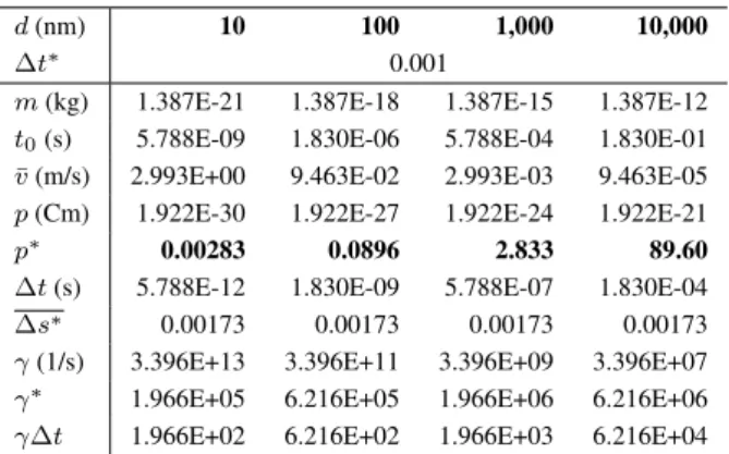
We change two parameters in this analysis, the par- ticle diameter, d, and the reduced time step, ∆t∗. Ac- cording toEq. 2, the dipole moment can be written as p=Kd3, whereK = 1.922×10⁻⁶Cm−2for the pa- rameters inTable 2.Table 3 contains various quantities computed for different values ofd.
It is seen thatp∗falls into the regime simulated in this study aroundd= 1µm. For diameters below100nm, at least, at the present value ofK, the reduced dipole mo- ment is too weak to counterbalance the thermal motion and to produce considerable chain formation.
The reduced friction coefficient also depends ond; it increases withd1/2. It is in the regime ofγ∗≈105−106. This looks simulatable, though it will require consider- able computer time, because∆t∗is limited. The param- eter ∆s∗ is the same for every diameter; it practically equivalent to∆t∗. To look at the effect of∆t∗, we show the same data for varying∆t∗ at a fixedd(100nm) in Table 4.
Table 3: Change of various variables as the diameter of spheres is changed from10to10,000nm for time step
∆t∗= 0.001.
d(nm) 10 100 1,000 10,000
∆t∗ 0.001
m(kg) 1.387E-21 1.387E-18 1.387E-15 1.387E-12 t0(s) 5.788E-09 1.830E-06 5.788E-04 1.830E-01
¯
v(m/s) 2.993E+00 9.463E-02 2.993E-03 9.463E-05 p(Cm) 1.922E-30 1.922E-27 1.922E-24 1.922E-21
p∗ 0.00283 0.0896 2.833 89.60
∆t(s) 5.788E-12 1.830E-09 5.788E-07 1.830E-04
∆s∗ 0.00173 0.00173 0.00173 0.00173
γ(1/s) 3.396E+13 3.396E+11 3.396E+09 3.396E+07 γ∗ 1.966E+05 6.216E+05 1.966E+06 6.216E+06 γ∆t 1.966E+02 6.216E+02 1.966E+03 6.216E+04
Table 4:Change of various variables as the reduced time step∆t∗is changed from0.0001to0.1for diameterd= 100nm.
d(nm) 100
∆t∗ 0.0001 0.001 0.01 0.1
m(kg) 1.387E-18 1.387E-18 1.387E-18 1.387E-18 t0(s) 1.830E-06 1.830E-06 1.830E-06 1.830E-06
¯
v(m/s) 9.463E-02 9.463E-02 9.463E-02 9.463E-02 p(Cm) 1.922E-27 1.922E-27 1.922E-27 1.922E-27
p∗ 0.0896 0.0896 0.0896 0.0896
∆t 1.830E-10 1.830E-09 1.830E-08 1.830E-07
∆s∗ 0.000173 0.00173 0.0173 0.173
γ(1/s) 3.396E+11 3.396E+11 3.396E+11 3.396E+11 γ∗ 6.216E+05 6.216E+05 6.216E+05 6.216E+05 γ∆t 6.216E+01 6.216E+02 6.216E+03 6.216E+04
6. Results and Discussion
In this study, we use a relatively small number of particles (N = 128) in order to save on computer time and be able to explore a wide range of parameters in reduced units.
We also fix the packing fraction expressed in term of the reduced density atρ∗ = 0.05. At these values the width of the simulation cell isL= 13.68d.
The computer code has been written (in Fortran) in a way that we performM0 time steps in the absence of applied electric field (E0= 0), andMEtime steps in the presence of it. That way, we can study the dynamics of chain formation after the electric field is switched on. To improve statistics, we can perform several of thisMc = M0+MEcycles and average over the cycles.
When we start a cycle over, we can choose between two options. We can either continue the simulation from the previous phase state point (configurations and veloci- ties) only without dipoles, or we can restart from a freshly generated initial configuration. In this work, we choose the second option. This choice ensures that we start the simulation with nonzero E0 in a completely disordered state without chains. The first option makes it possible to study the dynamics of the deconstruction of the chains.
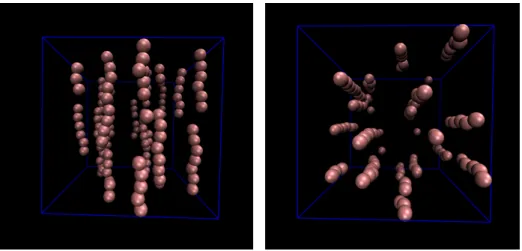
Figure 4:Typical snapshot of a simulation from the front (perpendicular to thezaxis, left panel) and top (parallel to thez axis, right panel) for a state when chains are formed.
6.1 Quantities studied
As the chains are being formed, certain physical quan- tities change, so they directly or indirectly character- ize chain formation quantitatively. In chains, particles are aligned into head-to-tail position along thez-axis as shown inFig. 4. There are longer and shorter chains and the distribution of chains of various lengths changes con- tinuously as the simulation evolves.
Since the head-to-tail position is the lowest energy configuration of the ER spheres (seeFig. 2andEqs. 24 and25), the average one-particle dipole-dipole energy, huDDib/kT, is a good indicator of chain formation. As it turns out, it is the best converging indicator.
By average, we mean average over a block in the sim- ulation, denoted byh. . .ib. The length of a block (Mbis the number of time steps in a block), again, is a subject of optimization. If a block is too short, the physical quan- tities averaged over a block will have bad statistics. If a block is too long, we loose information about the dynam- ics of the system.
Diffusion constant When the particles are “frozen”
into chains, their mobility decreases. Chains are frozen only at very large dipole moments, when even colum- nar structures are formed. In a moderate range of(p∗)2, chains move around, break apart, and rejoin, see the video clip at https://youtu.be/OwXsuz6p0W4.
A snapshot of this video clip is shown inFig. 5.
The isotropic diffusion constant is computed as the slope of the mean square displacement (MSD) as a func- tion of time:
Db= hr2(t)ib
2tb
, (30)
where h. . .ib denotes an average over time steps in a block and particles and tb is the length of the block in time. The exact equilibrium diffusion constant is obtained in the limit oftb→ ∞.
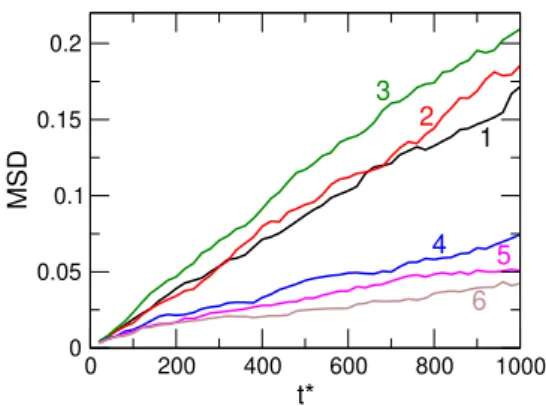
Here, we must be satisfied with an approximate value of Db obtained over a block of limited length. Fig. 6 shows the MSD as a function oft∗ for six equidistantly chosen blocks. In this particular case,γ∗ = 5000, so the slope isD∗ = MSD/t∗b≈0.0002for the WCA fluid as
Figure 5:A snapshot of the video clip athttps://youtu.be/OwXsuz6p0W4.
0 200 400 600 800 1000 t*
0 0.05 0.1 0.15
0.2
MSD
1 2 3
4 5
6
Figure 6:The mean square displacement for six selected blocks. The blocks are selected in equidistant time peri- ods in way that the first three belong to theE= 0phase, while the second three belongs to the ER phase. Parame- ters:(p∗)2= 6,γ∗= 5,000,∆t∗= 0.02,Mb= 50,000.
also expressed by the Einstein relation (D∗ = 1/γ∗,Eq.
28). Here, the time-length of the block ist∗b= ∆t∗Mb= 1,000, because∆t∗ = 0.02andMb= 50,000. The first three lines are in the E = 0regime, while the second three lines are in the ER regime. The slope apparently is smaller in the ER case than in the WCA case, but the scattering is large.
The sampling can be improved by averaging over cy- cles, but this does not help on the problem of the diffu- sion constant being approximate obtained for a too short block.
Chain length distributions The chain formation can be directly followed by identifying chains in every con- figuration. If that is done, we can obtain the number of chains,ns, having lengths. The average chain length can be computed as
l= P
ssns P
sns
. (31)
10000 20000 30000 40000 50000 t*
2 4 6 8 10
Average chain length
λe=0.5 λe=0.7 λg=1.1 λg=1.2
Figure 7:The trend of the change in the average chain length with various definitions of a chain: energetic with λe = 0.5and0.7, geometrical withλg = 1.1and1.2.
Parameters: (p∗)2 = 6, γ∗ = 10,000, ∆t∗ = 0.01, Mb= 10,000.
5 10 15 20
Chain length 0
1 2 3 4 5
Chain length distribution
10000 < t* < 250000 25000 < t* < 65000 65000 < t* < 100000
Figure 8: Chain length distribution averaged over three time intervals at the beginning (10,000< t∗ <25,000), in the middle (25,000 < t∗ < 65,000), and at the end (65,000< t∗<100,000) of chain formation. Parameters are the same as atFig. 7.
This quantity than can be averaged over time steps in a block, so chain formation can be followed by plotting the average chain length,hlib, as a function of time in steps oft∗b.
A chain, however, can be defined in various ways.
One simple definition is geometrical. If two particles are closer to each other than a predefined distance:
rij< λgd, (32) they are said to be part of the same chain. Another defi- nition is energetic. If the dipole-dipole interaction energy is smaller than a predefined threshold:
uDDij (rij, θ)< λeu0, (33) then they are said to be part of the same chain, whereu0 is the DD interaction energy in the head-to-tail position (Eq. 24).
Fig. 7shows the increase of the average chain length as a function of time as obtained from different chain def- initions and thresholdsλeandλg. In general, the trends as shown by the various definitions are the same. The dy- namic process of chains breaking up and reforming have the same effect in the cases of the various definitions.
This process can be characterized by time constants ob- tained from fitting exponential functions. These time con- stants are insensitive to the choice of the chain definition.
Here, we will use the geometrical definition with the pa- rameterλg = 1.2. The geometrical definition is advan- tageous, because it can also be used in the absence of an electric field.
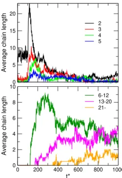
The average chain length is an informative, but aver- aged quantity. From the simulations, we have the more detailed ns vs. s chain length distributions that give the average number of chains of different lengths as a function of s. This function varies with time, see the video clip at https://youtu.be/OwXsuz6p0W4.
To show the dynamics of this function, we average it for three distinct time intervals. The first one refers to the
0 200 400 600 800 1000 t*
0 2 4 6 8 10
Average chain length
6-12 13-20 21- 0
5 10 15 20
Average chain length
2 3 4 5
Figure 9:The variation of the number of chains of vari- ous lengths in time. Top: chains of lengths2,3,4, and5.
Bottom: number of chains belonging to the ranges6−12, 13−20, and above21. Parameters are the same as atFig.
7.
beginning of the time period in the presence of the field when the chains start forming. In the second, intermedi- ate time interval (25,000 < t∗ < 65,000) longer chains are formed, while in the third time interval (65,000 <
t∗ < 100,000), full chains crossing the simulation box are formed.
Fig. 8shows these three time-averaged functions. At the beginning, there are many pairs and short chains (black curve). In the intermediate time interval, the num- ber of short chains decreases and longer chains are formed. In the third time interval, a well-defined peak at s= 14appears that corresponds to the full chains cross- ing the simulation box of lengthL= 13.68d.
We can get a much better impression of the dynam- ics of chain formation, if we plot ns as a function of time. Because there are too many possiblens numbers to plot, again, we average over certain regions of chain lengths as seen inFig. 9. In the top panel, the behavior of short chains from pairs tos= 5is shown. The behavior of these chains is qualitatively similar. First, as the elec- tric field is switched on, their numbers increase abruptly, then, as longer chains absorb them, or they fuse into longer chains, their numbers gradually decreases. Practi- cally, they behave like reactive intermediates in chemical reactions: their formation is a first necessary step towards the formation of the end products.
The number of chains whose lengths are between 6 and 12 (bottom panel) behaves similarly. The curve for the chains whose lengths are between 13 and 20, how- ever, saturates aroundns = 4. This means that there are
1 2 3 4 5 6
r*
1 10
Radial distribution function
0 < t* < 10000 10000 < t* < 25000 25000 < t* < 65000 65000 < t* < 100000
Figure 10: Radial distribution functions averaged over four time intervals in the absence of the electric field (0<
t∗<10,000), at the beginning (10,000< t∗<25,000), in the middle (25,000 < t∗ < 65,000), and at the end (65,000< t∗<100,000) of chain formation. Parameters are the same as atFig. 7.
generally about4 full chains in the simulation box (this value, of course, depends on system size and packing fraction). They are often accompanied by shorter chains as seen inFig. 4and the video clip.
Chains longer than 20 also exist. It can also occur that two chains are stuck together. Whether it is a stable, long time-span configuration, depends on the strength of the dipole moment (the electric field, in reality). A par- ticle is attracted to another particle in a chain, if they are aligned in a way that θ = π/4, see Fig. 2. This is a relatively weak attraction compared to the head-to-tail position. The chains displace due to thermal motion, so the chains move out of these mutual positions that favors aggregation of chains. If two chains move in a way that the particles get next to each other (θ = π/2), a repul- sive force replaces the weak attractive one. So, a strong dipole moment is needed to overcome the thermal motion if we want to see stable columnar aggregations of chains as seen many times in the literature.
Pair distribution functions As particles aggregate into chains, the structure of the fluid, generally expressed with pair distribution functions, changes. In an anisotropic dipolar fluid, we generally use the series expansion of the pair correlation function of axially symmetric molecules as
g(ij) =X
nml
hmnl(rij)umnl(ij). (34) This expansion separates distance and angular depen- dence in such a way that the projections hmnl(rij)de- pend only on the distance of particles and the projections umnl(ij)are rotational invariants.
The projectiong(rij) =h000(rij)is the usual radial distribution function (RDF):
g(rij) = Z
g(ij)dΩidΩj, with u000= 1, (35)
0 1 2 3 4 5 6 r*
1 10 100
RDF in the xy plane
0 < t* < 10000 10000 < t* < 25000 25000 < t* < 65000 65000 < t* < 100000
Figure 11:Thexy-plane radial distribution functions av- eraged over four time intervals as inFig. 10. Parameters are the same as atFig. 7.
whereΩidenotes molecular orientation. In a fluid phase, h000(rij) → 1 when rij → ∞ both in isotropic and anisotropic phases. Other projections, called angular cor- relation functions, can also characterize chain formation, but we will discuss only the RDF in this study.
Similar toFig. 8, we plot the RDF averaged over the time intervals discussed at the chain length distributions.
In addition to those three time intervals, we also consider the time interval0< t∗<10,000here, which is the time of the electric field being switched off.Fig. 10shows that theg(r)function behaves like a typical RDF for a dense real gas (ρ∗= 0.05) in the absence ofE0.
As the electric field is switched on, however, larger and larger peaks appear as time goes by and longer and longer chains are formed. The peaks appear at every integer multiples of d values that correspond to parti- cles in the chain. A more detailed behavior ofg(r)can be followed in the video clip:https://youtu.be/
OwXsuz6p0W4.
When the chains are formed, they are relatively stable, but they diffuse around in thexy plane. Therefore, we also define the RDF in thexy plane to follow how the chains are distributed over thexyplane. We will denote it withgxy(r)and is calculated the same way as the three- dimensional RDF.
Fig. 11shows these functions averaged over the time periods as inFig. 10. A similar conclusion can be drawn as from that figure except that the first peak now appears atr∗ = 0, where now r = p
∆x2+ ∆y2. This peak represents particles belonging to the same chain. Peaks represent probable distances between chains. The shape of the curve indicates that this ER system ((p∗)2 = 6) behaves like a two-dimensional fluid of chains.
At a given time (or, in a given block), these series of peaks are absent. Snapshots of gxy(r) show where the chains are in a given moment. This can be followed in the video clip:https://youtu.be/OwXsuz6p0W4. The gxy(r) function averaged over a longer time pe- riod characterizes the behavior of the chains as a two- dimensional fluid.
-10 -5 0
Dipole-dipole energy / kT
0.6 0.8 1 1.2
D / D(E=0)
0 5×10⁴ 1×10⁵ 2×10⁵ 2×10⁵ 5
10 15
Average chain length
∆t*=0.005
∆t*=0.01
∆t*=0.02 (µ*)2=6
γ*=10000
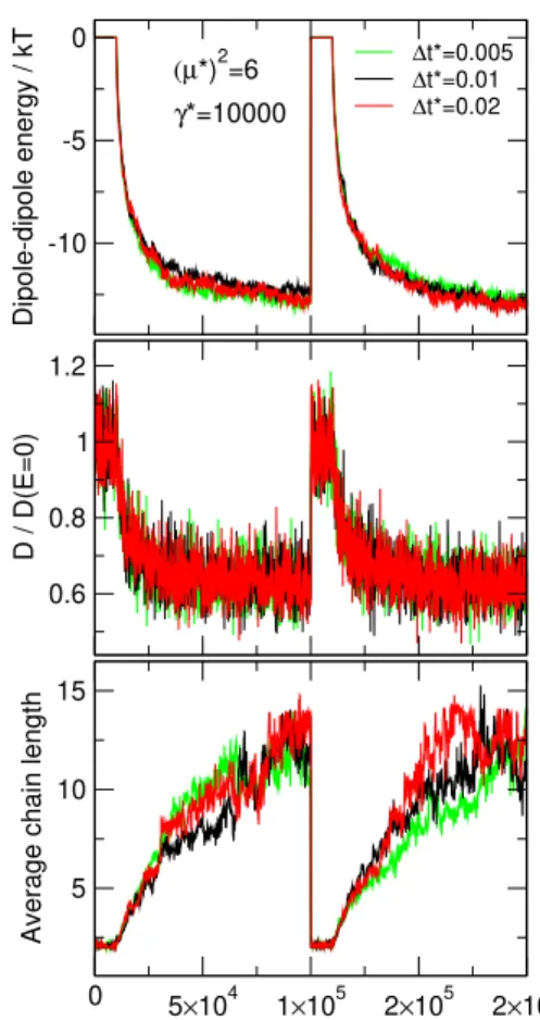
Figure 12: The one-particle dipole-dipole energy (top panel), the diffusion constant relative to its value in the ab- sence ofE0(middle panel), and the average chain length (geometrical definition withλg = 1.2, bottom panel) as functions of time using different time steps. Parameters:
(p∗)2= 6andγ∗= 10,000. TheMbis changed in a way that∆t∗×Mbis constant.
6.2 The effect of time step
First, let us consider the effect of the choice of the time step,∆t∗.Fig. 12shows the variation of the one-particle dipole-dipole energy, the diffusion constant, and the aver- age chain length (geometrical definition withλg = 1.2) for different values of∆t∗. The length of a block mea- sured int∗is kept fixed. It is seen that the measured quan- tities behave the same way as a function of time, which indicates that the BD simulation algorithm is robust and provides results that are independent of the time step.
Also, we monitored the temperature computed from the kinetic energy, hTi = mhv2i/3k, and found that the algorithm reproduces the prescribed temperature very precisely even for this highly anisotropic fluid. This sup- ports the claim of the developers that this algorithm pro- vides a very good Langevin thermostat [24–26].
If we change∆t∗, but we keepMbat the same value, meaning that we change the time length of the block, the dipole-dipole energy and the average chain length are still insensitive to the choice of ∆t∗ (data not shown). The diffusion coefficient, however, changes with the length of the blocks as already discussed above (at Fig. 6). This
-10 -5 0
Dipole-dipole energy / kT
γ*=1000 γ*=2000 γ*=5000 γ*=10000
0.2 0.4 0.6 0.8 1 1.2
D / D(E=0)
0 5×10⁴ 1×10⁵ 2×10⁵ 2×10⁵ 5
10 15 20
Average chain length
(µ*)2=6
∆t*=0.01
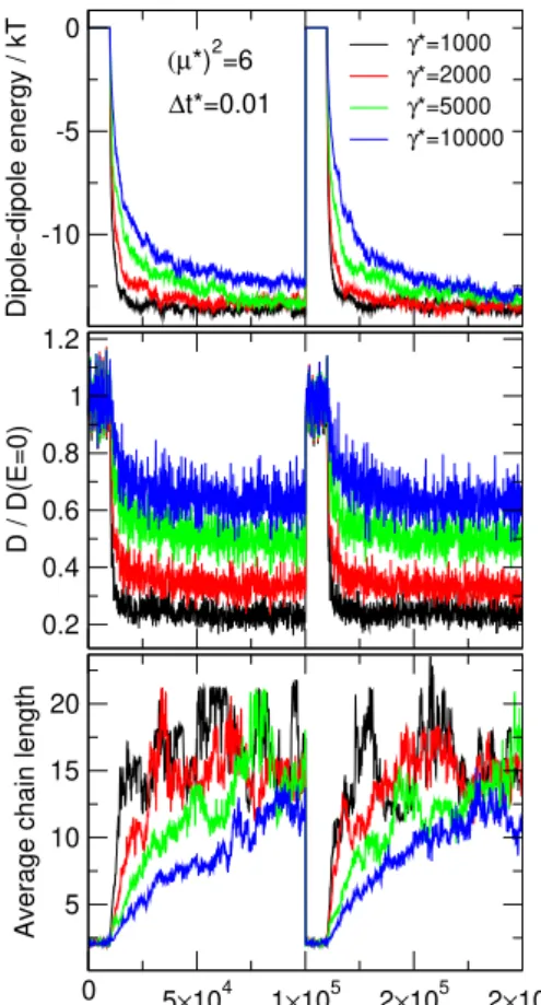
Figure 13: The one-particle dipole-dipole energy (top panel), the diffusion constant relative to its value in the ab- sence ofE0(middle panel), and the average chain length (geometrical definition withλg = 1.2, bottom panel) as functions of time using different friction coefficients. Pa- rameters:(p∗)2= 6and∆t∗= 0.01.
means that we have a trade-off between satisfactory sam- pling over a block and good resolution in time.
We do not consider viscosity in this paper; we refer it to future studies. This trade-off will be present in the case of the viscosity (and the stress tensor) as well. It will be even more serious, because the viscosity is even a more poorly converging quantity than the diffusion constant.
6.3 The effect of friction coefficient
We fix the dipole moment at(p∗)2= 6and the time step at∆t∗ = 0.01, and change the friction coefficient from γ∗ = 1,000to10,000. As discussed in the next section, realistic ER fluids have friction coefficients even larger than10,000, but we refer studying that regime to future publications.
Asγ∗ is increased, the curves tend to their equilib- rium values asE0 is switched on at a lower rate. Fitting exponential functions to these curves and identifying pro- cesses of different time lengths as parts of the complex process of chain formation will also be the subject of fu- ture studies.
The change inγ∗does not influence the value where the energy and the average chain length converge to.
-12 -10 -8 -6 -4 -2 0
Dipole-dipole energy / kT
(p*)2=2 (p*)2=4 (p*)2=6
0.5 0.6 0.7 0.8 0.9 1 1.1
D / D(E=0)
0 5×10⁴ 1×10⁵ 2×10⁵ 2×10⁵ 5
10 15
Average chain length
∆t*=0.01 γ*=10000
6
6 6
4
4 2
2
2
Figure 14: The one-particle dipole-dipole energy (top panel), the diffusion constant relative to its value in the ab- sence ofE0(middle panel), and the average chain length (geometrical definition withλg = 1.2, bottom panel) as functions of time using different dipole moments. Param- eters:γ∗ = 10,000and∆t∗ = 0.01. This figure shows twoM0+MEcycles.
They converge to the same value but with a different rate.
Changing friction, however, changes the diffusion con- stant.Fig. 13shows the diffusion constant relative to its value in the absence of the field computed asD∗= 1/γ∗. The diffusion constant decreases to a smaller value rela- tive toD∗(E= 0)at smaller values ofγ∗.
The average chain length shows that smaller γ∗ re- sults in a more wildly fluctuating system than a largerγ∗. The particles diffuse faster and produce larger variations in configurations during a given time period.
6.4 The effect of dipole moment
Our simulations show (Fig. 14) that the quantity that determines the structure of the ER fluid is the reduced dipole moment, namely, the relation of the dipole-dipole energy to the thermal energy unit,kT.Fig. 14shows that these quantities converge to their equilibrium values ex- hibiting a similar trend.
The dipole moments studied in this work belong to the regime where the ER fluid considered as a collection of chains is still a fluid, namely, it does not solidify. Sev- eral papers in the literature study solidification of the ER
chains [5,6,15,16,22].
7. Summary
In this work, we use a newly developed integrator algo- rithm to solve the Langevin equations and to perform BD simulations for ER fluids. Our focus was on the method- ological development and identifying appropriate system parameters through which we can follow the dynamics of chain formation in the system.
The usefulness of computer simulations lies not only in the fact that we can follow the particles’ trajectories, but also in the fact that we can gain a profound amount of information from these trajectories. In the BD simula- tions, for example, we can follow how the average num- ber of chains of varying lengths changes in time. From that detailed information we can deduce time constants for characteristic processes during chain formation.
We intend to dig into those details in subsequent stud- ies. Also, we want to examine the behavior of the chains under a stress.
Acknowledgement
This research was supported by the European Union, co- financed by the European Social Fund. EFOP-3.6.2-16- 2017-00002. We also acknowledge the support of the Na- tional Research, Development and Innovation Office – NKFIH K124353.
REFERENCES
[1] Winslow, W.M.: Induced Fibration of Suspensions, J. Appl. Phys., 1949, 20(12), 1137–1140 DOI:
10.1063%2F1.1698285
[2] Duclos, T.G.; Carlson, J.D.; Chrzan, M.J.; Coul- ter, J.P.: Electrorheological Fluids — Materials and Applications, in Solid Mechanics and Its Applica- tions (Springer Netherlands), 1992, 13, 213–241
DOI: 10.1007%2F978-94-017-1903-2_5
[3] Havelka, K.O.; Filisko, F.E. (eds.): Progress in Electrorheology (Springer US), 1995. DOI:
10.1007%2F978-1-4899-1036-3
[4] Klingenberg, D.J.; van Swol, F.; Zukoski, C.F.:
Dynamic simulation of electrorheological suspen- sions, J. Chem. Phys., 1989, 91(12), 7888–7895
DOI: 10.1063%2F1.457256
[5] Heyes, D.M.; Melrose, J.R.: Brownian Dynamics Simulations of Electro-Rheological Fluids, II: Scal- ing Laws, Mol. Sim., 1990, 5(5), 293–306 DOI:
10.1080%2F08927029008022415
[6] Whittle, M.: Computer simulation of an electrorhe- ological fluid, J. Non-Newtonian Fluid Mechan- ics, 1990, 37(2-3), 233–263 DOI: 10.1016%2F0377- 0257%2890%2990007-x
[7] Klingenberg, D.J.; Zukoski, C.F.: Studies on the steady-shear behavior of electrorheological suspensions, Langmuir, 1990, 6(1), 15–24 DOI:
10.1021%2Fla00091a003
[8] Jaggi, N.K.: Structure and dynamics of a dense dipolar system in an electric field and their rel- evance to electrorheological fluids,J. Stat. Phys., 1991,64(5-6), 1093–1102DOI: 10.1007%2Fbf01048816
[9] See, H.; Doi, M.: Aggregation Kinetics in Electro- Rheological Fluids, J. Phys. Soc. Japan, 1991, 60(8), 2778–2782DOI: 10.1143%2Fjpsj.60.2778
[10] Bonnecaze, R.T.; Brady, J.F.: Dynamic simulation of an electrorheological fluid,J. Chem. Phys., 1992, 96(3), 2183–2202DOI: 10.1063%2F1.462070
[11] Toor, W.R.: Structure Formation in Electrorheologi- cal Fluids,J. Colloid Interf. Sci., 1993,156(2), 335–
349DOI: 10.1006%2Fjcis.1993.1121
[12] Hass, K.C.: Computer simulations of nonequilib- rium structure formation in electrorheological flu- ids, Phy. Rev. E, 1993, 47(5), 3362–3373 DOI:
10.1103%2Fphysreve.47.3362
[13] Tao, R.; Jiang, Q.: Simulation of structure formation in an electrorheological fluid,Phys. Rev. Lett., 1994, 73(1), 205–208DOI: 10.1103%2Fphysrevlett.73.205
[14] Tao, R.; Jiang, Q.: Simulation of Solid Structure Formation in an Electrorheological Fluid, Int. J.
Modern Phys. B, 1994,08(20n21), 2721–2730DOI:
10.1142%2Fs0217979294001081
[15] Baxter-Drayton, Y.; Brady, J.F.: Brownian elec- trorheological fluids as a model for flocculated dis- persions,J. Rheology, 1996,40(6), 1027–1056DOI:
10.1122%2F1.550772
[16] Gulley, G.L.; Tao, R.: Structures of an electrorheo- logical fluid,Phys. Rev. E, 1997,56(4), 4328–4336
DOI: 10.1103%2Fphysreve.56.4328
[17] Jian, L.; Jiapeng, S.: Simulation of a three- dimensional electrorheological suspension, J. Appl. Phys., 1996, 79(9), 7312–7317 DOI:
10.1063%2F1.361447
[18] Wang, B.; Liu, Y.; Xiao, Z.: Dynamical modelling of the chain structure formation in electrorheolog- ical fluids,Int. J. Eng. Sci., 2001, 39(4), 453–475
DOI: 10.1016%2Fs0020-7225%2800%2900054-9
[19] Enomoto, Y.; Oba, K.: Simulation of structures and their rheological properties in electrorheologi- cal fluids,Physica A, 2002, 309(1–2), 15–25 DOI:
10.1016%2Fs0378-4371%2802%2900599-x
[20] Climent, E.; Maxey, M.R.; Karniadakis, G.E.: Dy- namics of Self-Assembled Chaining in Magne- torheological Fluids,Langmuir, 2004,20(2), 507–
513DOI: 10.1021%2Fla035540z
[21] Cao, J.G.; Huang, J.P.; Zhou, L.W.: Structure of Electrorheological Fluids under an Electric Field and a Shear Flow: Experiment and Computer Sim- ulation,J. Phys. Chem. B, 2006, 110(24), 11635–
11639DOI: 10.1021%2Fjp0611774
[22] Domínguez-García, P.; Melle, S.; Pastor, J.M.; Ru- bio, M.A.: Scaling in the aggregation dynamics of a magnetorheological fluid,Phys. Rev. E, 2007,76(5), 051403DOI: 10.1103%2Fphysreve.76.051403
[23] Heyes, D.M.: Rheology of molecular liquids and concentrated suspensions by microscopic dynami-
cal simulations,J. Non-Newton. Fluid, 1988,27(1), 47–85DOI: 10.1016%2F0377-0257%2888%2980004-1
[24] Grønbech-Jensen, N.; Farago, O.: A simple and effective Verlet-type algorithm for simulating Langevin dynamics,Mol. Phys., 2013,111(8), 983–
991DOI: 10.1080%2F00268976.2012.760055
[25] Farago, O.: Langevin thermostat for robust configu- rational and kinetic sampling,Physica A, 2019,534, 122210DOI: 10.1016%2Fj.physa.2019.122210
[26] Jensen, L.F.G.; Grønbech-Jensen, N.: Accurate con- figurational and kinetic statistics in discrete-time Langevin systems, Mol. Phys., 2019, 117(18), 2511–2526DOI: 10.1080%2F00268976.2019.1570369
[27] Sherman, S.G.; Paley, D.A.; Wereley, N.M.: Mas- sively Parallel Simulations of Chain Formation and Restructuring Dynamics in a Magnetorheological Fluid, in ASME 2011 Conference on Smart Mate- rials, Adaptive Structures and Intelligent Systems, Volume 1 (ASMEDC), DOI: 10.1115%2Fsmasis2011- 5188
[28] Sherman, S.G.; Paley, D.A.; Wereley, N.M.: Paral- lel Simulation of Transient Magnetorheological Di- rect Shear Flows Using Millions of Particles,IEEE Transactions on Magnetics, 2012, 48(11), 3517–
3520DOI: 10.1109%2Ftmag.2012.2201214
[29] Fernández-Toledano, J.C.; Ruiz-López, J.A.;
Hidalgo-Álvarez, R.; de Vicente, J.: Simulations of polydisperse magnetorheological fluids: A structural and kinetic investigation, J. Rheology, 2015,59(2), 475–498DOI: 10.1122%2F1.4906544
[30] Boda, D.; Valiskó, M.; Szalai, I.: The origin of the interparticle potential of electrorheological flu- ids, Cond. Matt. Phys., 2013, 16(4), 43002 DOI:
10.5488/cmp.16.43002
[31] Jackson, J.D.: Classical Electrodynamics (Wiley, New York), 3rd edn., 1999.ISBN: 978-0471309321
[32] Boda, D.; Gillespie, D.; Nonner, W.; Henderson, D.; Eisenberg, B.: Computing induced charges in inhomogeneous dielectric media: Application in a
Monte Carlo simulation of complex ionic systems, Phys. Rev. E, 2004,69(4), 046702DOI: 10.1103/phys- reve.69.046702
[33] Lemons, D.S.; Gythiel, A.: Paul Langevin’s 1908 paper “On the Theory of Brownian Motion” [“Sur la théorie du mouvement brownien,” C. R. Acad. Sci.
(Paris) 146, 530–533 (1908)],Am. J. Phys., 1997, 65(11), 1079–1081DOI: 10.1119%2F1.18725
[34] Schneider, T.; Stoll, E.: Molecular-dynamics study of a three-dimensional one-component model for distortive phase transitions, Phys. Rev. B, 1978, 17(3), 1302–1322DOI: 10.1103%2Fphysrevb.17.1302
[35] van Gunsteren, W.; Berendsen, H.: Algorithms for brownian dynamics,Mol. Phys., 1982,45(3), 637–
647DOI: 10.1080%2F00268978200100491
[36] Brünger, A.; Brooks, C.L.; Karplus, M.: Stochas- tic boundary conditions for molecular dynam- ics simulations of ST2 water, Chem. Phys.
Lett., 1984, 105(5), 495–500 DOI: 10.1016%2F0009- 2614%2884%2980098-6
[37] Leimkuhler, B.; Matthews, C.: Rational Construc- tion of Stochastic Numerical Methods for Molec- ular Sampling, Appl. Math. Res. eXpress, 2013, 2013(1), 34–56DOI: 10.1093%2Famrx%2Fabs010
[38] Horváth, B.; Szalai, I.: Structure of electrorhe- ological fluids: A dielectric study of chain for- mation, Phys. Rev. E, 2012, 86(6),061403 DOI:
10.1103%2Fphysreve.86.061403
[39] Horváth, B.; Szalai, I.: Dynamic dielectric response of electrorheological fluids in drag flow, Phys.
Rev. E, 2015, 92(4), 042308 DOI: 10.1103%2Fphys- reve.92.042308
[40] Berti, C.; Furini, S.; Gillespie, D.; Boda, D.;
Eisenberg, R.S.; Sangiorgi, E.; Fiegna, C.: A 3- D Brownian Dynamics simulator for the study of ion permeation through membrane pores, J.
Chem. Theor. Comput., 2014, 10(8), 2911–2926
DOI: 10.1021/ct4011008
![Table 2: Experimental parameters [38, 39]. in 4 out 2.7 η (Pa s) 0.5 E 0 (V/m) 10 6 T (K) 300 ρ out (kg/m 3 ) 2650](https://thumb-eu.123doks.com/thumbv2/9dokorg/782084.36047/5.892.209.349.118.240/table-experimental-parameters-in-out-η-pa-out.webp)