Decentralized machine learning using compressed push-pull averaging
Gábor Danner
danner@inf.u-szeged.hu University of Szeged
Szeged, Hungary
István Hegedűs
ihegedus@inf.u-szeged.hu University of Szeged
Szeged, Hungary
Márk Jelasity
jelasity@inf.u-szeged.hu University of Szeged, and MTA-SZTE
Research Group on AI Szeged, Hungary
Abstract
For decentralized learning algorithms communication effi- ciency is a central issue. On the one hand, good machine learning models require more and more parameters. On the other hand, there is a relatively large cost for transferring data via P2P channels due to bandwidth and unreliability issues. Here, we propose a novel compression mechanism for P2P machine learning that is based on the application of stateful codecs over P2P links. In addition, we also rely on transfer learning for extra compression. This means that we train a relatively small model on top of a high quality pre-trained feature set that is fixed. We demonstrate these contributions through an experimental analysis over a real smartphone trace.
CCS Concepts:• Computing methodologies → Ma- chine learning; •Networks→Peer-to-peer protocols;
•Computer systems organization→Peer-to-peer ar- chitectures.
Keywords:decentralized averaging, compressed communi- cation, machine learning
ACM Reference Format:
Gábor Danner, István Hegedűs, and Márk Jelasity. 2020. De- centralized machine learning using compressed push-pull averaging. In 1st International Workshop on Distributed In- frastructure for Common Good (DICG ’20), December 7–11, 2020, Delft, Netherlands. ACM, New York, NY, USA, 6 pages.
https://doi.org/10.1145/3428662.3428792
1 Introduction
We are witnessing an increased interest in machine learn- ing solutions that do not require data collection at a central location [21]. Federated learning, for example, has been de- veloped and deployed by Google to be able to exploit user data without violating data privacy [13,16].
ACM acknowledges that this contribution was authored or co-authored by an employee, contractor or affiliate of a national government. As such, the Government retains a nonexclusive, royalty-free right to publish or reproduce this article, or to allow others to do so, for Government purposes only.
DICG 2020, December 07–11 , 2020, Delft, The Netherlands
© 2020 Association for Computing Machinery.
ACM ISBN 978-1-4503-8197-0/20/12. . . $15.00 https://doi.org/10.1145/3428662.3428792
Within this area, solutions that are even more radically decentralized, such as gossip learning [18], are promising candidates to support applications for the common good [5].
The reason is that these solutions can be deployed literally without any investment at all, relying only on user devices and no additional infrastructure, without any pressure to make a profit.
In this paper, we propose a novel variant of gossip learn- ing that uses codec-based compression to increase the com- munication efficiency. Compression methods have been studied in depth in the context of simpler computations such as averaging [6,9,15,23]. In the context of machine learning, federated learning solutions also use compression [13,20]
but the actual averaging is performed centrally. Koloskova et al. have a similar focus to our paper but they apply only simple stateless quantization [12].
Our contribution in this paper is twofold. First, we adapt the compressed push-pull averaging algorithm from [7] for gossip learning, and achieve a higher communication effi- ciency than previous methods based on subsampling. Sec- ond, we evaluate the solution over datasets including a transfer learning dataset, thereby demonstrating that it is feasible to adapt pre-existing deep neural network models to another domain by training only their last layer, which makes them accessible for gossip learning applications.
2 Background
We give a short overview of some of the concepts and ideas used here taken from machine learning and gossip learning.
2.1 Machine Learning: Classification
In the classification problem, a data set is given that con- tains examples in the form(𝑥𝑖, 𝑦𝑖) ∈ D, where𝑖∈ {1, . . . , 𝑛}.
Here𝑥 ∈R𝑑is a𝑑dimensional real vector (the so-called fea- ture vector) that represents the a sample from the data set D, and𝑦𝑖 ∈ Cis the corresponding class label. The prob- lem of supervised learning is to find the parameters (𝑤) of a functionF𝑤 :R𝑑→ C, that can correcly classify the sam- ples of the dataset. In addition, we expect that this function can classify any samples drawn from the same distribution as the data set as well. This property is called generalization.
One way to find the parameters of the above defined func- tion is to solve a minimization problem
𝑤∗=arg min
𝑤 𝐽(𝑤)= 1 𝑛
Õ𝑛
𝑖=1
ℓ(F𝑤(𝑥𝑖), 𝑦𝑖) +𝜆 2k𝑤k2, whereℓ()is a loss function (e.g., squared error) and k𝑤k2 is the regularization term with𝜆regularization coefficient.
Gradient descent is the most basic method that can be used to find𝑤∗. Here, the following iteration is expected to cov- erge to𝑤∗:
𝑤𝑡+1=𝑤𝑡−𝜂𝑡∇𝑤𝐽(𝑤𝑡)= 𝑤𝑡−𝜂𝑡(𝜆𝑤𝑡+ 1
𝑛 Õ𝑛
𝑖=1
𝜕ℓ(𝐹𝑤(𝑥𝑖), 𝑦𝑖)
𝜕𝑤 (𝑤𝑡)),
where ∇𝑤 is the gradient of the objective function in 𝑤, summed over the samples, and𝜂 is the learning rate. Sto- chastic gradient descent (SGD) computes the approximation of the gradient on only one sample at a time, taking different samples for each step:
𝑤𝑡+1=𝑤𝑡−𝜂𝑡(𝜆𝑤𝑡+ 𝜕ℓ(𝐹𝑤(𝑥𝑖), 𝑦𝑖)
𝜕𝑤 (𝑤𝑡)).
Logistic regression is a specific instantiation of the above abstract framework with
𝐽(𝑤)=−1 𝑛
Õ𝑛 𝑖=1
ln𝑃(𝑦𝑖|𝑥𝑖, 𝑤) +𝜆 2k𝑤k2,
where 𝑦𝑖 ∈ {0,1}, 𝑃(0|𝑥𝑖, 𝑤) = (1 + 𝑒𝑥𝑝(𝑤𝑇𝑥))−1 and 𝑃(1|𝑥𝑖, 𝑤) = 1−𝑃(0|𝑥𝑖, 𝑤). Usually a bias term (𝑏) is also added to the parameters and we have 𝑃(0|𝑥𝑖, 𝑤) = (1 + 𝑒𝑥𝑝(𝑤𝑇𝑥+𝑏))−1.
In this paper, we use logistic regression as our learning algorithm. However, as we desribe later, with transfer learn- ing we can effectively learn arbitrarily complex deep neural network models as well.
2.2 Gossip learning
Gossip Learning [18] is a decentralized learning algorithm, where a network of nodes is given. Each node stores a part of the data set (perhaps only one sample per node), and ma- chine learning models take random walks in the network while being updated on the nodes by the local training data.
The update step of the models can be done by the above de- scribed gradient method. The models can also be averaged in parallel to these update steps, which results in a signifi- cant speedup. This averaging is normally implemented by merging (weighted averaging) models locally.
We use partitioned token gossip learning as our base- line [11]. In this algorithm, the token account algorithm [8]
is applied to gossip learning with sampling-based compres- sion [10]. The model parameter vector is divided into pre- defined partitions that travel independently in the network.
Each partition has its own age that is used as a weight dur- ing merging.
In scenarios where the message transfer time is consid- erably shorter than the gossip cycle length, token accounts can improve the performance of gossip algorithms by form- ing rapid message chains, where information is propagated like a “hot-potato”, while still providing guarantees on amor- tized communication costs. In a nutshell, during each cycle, each node gets a token, while sending a message costs a to- ken. The more tokens a node has, the more eager it is to spend them, possibly sending freshly arrived information to more than one node, or sending a message proactively (to prevent the extinction of messages). In partitioned token gossip learning, each partition has its own token account.
2.3 Codec Basics
A codec can be used to encode and decode a series of real valued messages over a given directed link. It consists of an encoder and a decoder at the origin and the target of the link, respectively. We shall use the notations from [17]. En- coding (quantization) maps real values to a discrete alpha- bet𝑆, and decoding maps an element of alphabet𝑆back to a real value. Codecs may have a state (e.g. the last transmitted value). Every stateful codec implementation defines its own state spaceΞ(the same for the encoder and the decoder).
The encoder𝑄 : Ξ×R → 𝑆 maps a given real value to a quantized encoding based on the current local state of the encoder. The decoding function𝐾 : Ξ×𝑆 → Rmaps the encoded value back to a real value based on the current local state of the decoder. The state transition function𝐹 : Ξ×𝑆 → Ξ determines the dynamics of the state of the encoder and the decoder.
Although the encoder and the decoder are two remote agents that communicate over a limited link, we can ensure that both of them maintain an identical state, since the en- coder’s side can simulate the decoder locally, thus they can both perform identical state transitions, assuming the same initial state. If communication is not reliable, the algorithms using the codec must take additional measures to keep the states consistent.
3 Compressed push-pull learning
Our compressed push-pull learning algorithm is based on a compressed push-pull averaging protocol that compresses communication using codecs [7]. The nodes perodically train their model on the local data, as well as perform dis- tributed averaging of the models.
When used without model training, the algorithm falls back to computing the average of the initial 𝑤 vectors weighted by their respective initial𝑡values. This is achieved by simultaneously computing the average of𝑡𝑤and that of 𝑡, since the quotient of these is the weighted average of𝑤.
The pseudocode is shown in Algorithms1and2. The al- gorithm is local, hence the scope of the variables is limited to the current node.
Models are encoded before sending and decoded after be- ing received. During a push-pull transaction, the nodes ex- change their encoded models, then, based on the decoded models, a difference vector𝛿is computed on both sides that represents for each parameter the amount of mass being transferred in the push-pull exchange. Both nodes compute the same𝛿(with opposite signs), because they use only the information that was exchanged, ignoring the current, un- compressed local model𝑤. The difference is scaled by𝐻/2, where𝐻 ∈ (0,1]is a “greediness” parameter.𝐻 =1 results in the two nodes having equal values after the exchange, as- suming atomic (non-overlapping) push-pull exchanges and no compression. When these assumptions do not hold, a smaller𝐻is useful for stabilizing convergence. After decod- ing the models, the codec states are updated.
The techniques used for compression and ensuring sum preservation are largly unchanged from [7] and we do not go into great detail concerning these. One difference worth mentioning, though, is that we omitted the flow compensa- tion component, because it had a negative influence on the machine learning performance. Each push-pull exchange has an increasing unique ID, which is used to reject out-of- order push messages. If a push message is lost or rejected, neither side performs an update, so the network remains consistent. (Note thatupdaterefers to an averaging step, not to model training.) When node𝐵 accepts a push message from node𝐴, it performs an update, and sends back a pull message. If this arrives in time, the counterpart update is performed as well, the state of the network becoming con- sistent again. If the pull message is dropped or delayed then the update performed by𝐵needs to be reversed. This hap- pens when𝐵 receives the next push message from𝐴and learns (with the help of the update counter𝑢) that𝐴did not perform the counterpart update. The update is reversed us- ing the transfer saved in𝛿. Codec states are backed up and restored in a similar fashion.
Recall that we are averaging𝑡𝑤(and𝑡as well) across the network. During compression, however, we encode𝑤 in- stead of𝑡𝑤. This is because𝑡𝑤will surely not converge, but 𝑤 might, which is beneficial for adaptive codecs. Since𝑡is transmitted, the remote node can still compute an estimate for𝑡𝑤. In the messages, only the model𝑤 is compressed.
When𝑤is a large vector, the amortized cost of transmitting the other variables is negligible.
The algorithm works with any codec that is given by the definition of the state spaceΞ, the alphabet𝑆, and the functions 𝑄, 𝐹 and𝐾, as described previously. We apply these functions on the model parameter vector: the opera- tion is performed elementwise, each parameter having its own codec state. For each directed link(𝑗, 𝑖)there is a vec- tor of codecs for the direction 𝑗 →𝑖 as well as𝑗 ←𝑖. For the 𝑗 → 𝑖 direction, node 𝑗 stores the codec states (used for encoding push messages) in𝜉𝑖,𝑜𝑢𝑡,𝑙𝑜𝑐 and for the 𝑗 ←𝑖 direction the codecs (used for decoding pull messages) are
Algorithm 1Compressed push-pull learning (Part 1)
1: 𝑤is the local model.
2: 𝑡is the age of the local model.
3: 𝐷is the local data set.
4: 𝑢𝑖,𝑖𝑛 and𝑢𝑖,𝑜𝑢𝑡 record the number of times the local model was updated as a result of an incoming push or pull message from𝑖, respectively.
5: 𝑠𝑖andb𝑠𝑖are the encoded model and model age that were sent in the last push message to𝑖.
6: 𝛿𝑖,𝑜𝑢𝑡, 𝛿𝑖,𝑖𝑛are the last push, or pull parameter transfers to𝑖, respectively.
7: 𝛿b𝑖,𝑜𝑢𝑡,𝛿b𝑖,𝑖𝑛 are the last push, or pull age transfers to𝑖, respectively.
8: 𝑖𝑑𝑖 is the current unique ID created when sending the latest push message to𝑖, initially 0.
9: 𝑖𝑑𝑚𝑎𝑥,𝑖 is the maximal unique ID received in any push message from𝑖, initially−∞.
10: 𝜉𝑖,𝑖𝑛,𝑙𝑜𝑐, 𝜉𝑖,𝑖𝑛,𝑟𝑒𝑚, 𝜉𝑖,𝑜𝑢𝑡,𝑙𝑜𝑐, 𝜉𝑖,𝑜𝑢𝑡,𝑟𝑒𝑚 ∈ Ξare the states of the codecs for the local node and remote node𝑖, with initial values of𝜉0.
11: 𝜉𝑖,𝑖𝑛′,𝑙𝑜𝑐 and𝜉𝑖,𝑖𝑛′,𝑟𝑒𝑚 are the previous values of𝜉𝑖,𝑖𝑛,𝑙𝑜𝑐
and𝜉𝑖,𝑖𝑛,𝑟𝑒𝑚, with initial values of𝜉0.
12:
13: procedureonNextCycle ⊲Called everyΔtime units
14: (𝑤, 𝑡) ←train(𝑤, 𝑡, 𝐷)
15: 𝑖 ←randomOutNeighbor()
16: 𝑠𝑖 ←𝑄(𝜉𝑖,𝑜𝑢𝑡,𝑙𝑜𝑐, 𝑤) ⊲Model encoded and saved
17: b𝑠𝑖 ←𝑡
18: 𝑖𝑑𝑖 ←𝑖𝑑𝑖+1
19: send push message(𝑢𝑖,𝑜𝑢𝑡, 𝑠𝑖,b𝑠𝑖, 𝑖𝑑𝑖)to node𝑖
stored in𝜉𝑖,𝑜𝑢𝑡,𝑟𝑒𝑚at node𝑗. (Here, the subscript “out” indi- cates that the given codec is for the outgoing link.) Incoming link states are handled similarly.
4 Experiments
Now, we shall describe our experimental setup and our re- sults.
4.1 Datasets
We used two different datesets to evaluate our algorithm, and a third dataset used for our transfer learning approach, as we describe later. The main properties are shown in Table 1. The HAR (Human Activity Recognition Using Smartphones) database [1, 2] contains records that repre- sent movements from 6 different classes (walking, walk- ing_upstairs, walking_downstairs, sitting, standing, laying).
The data was collected from the smart phones of 30 differ- ent people, using the accelerometer, gyroscope and angular velocity sensors. High level features were extracted based on the frequency domain.
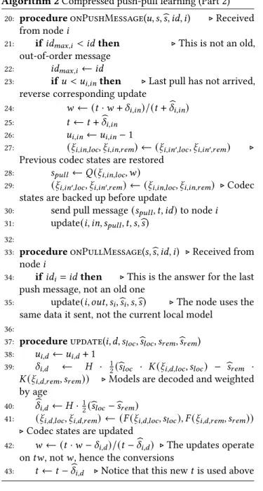
Algorithm 2Compressed push-pull learning (Part 2)
20: procedureonPushMessage(𝑢, 𝑠,b𝑠, 𝑖𝑑, 𝑖) ⊲Received from node𝑖
21: if𝑖𝑑𝑚𝑎𝑥,𝑖 <𝑖𝑑then ⊲This is not an old,
out-of-order message
22: 𝑖𝑑𝑚𝑎𝑥,𝑖 ←𝑖𝑑
23: if𝑢<𝑢𝑖,𝑖𝑛then ⊲Last pull has not arrived, reverse corresponding update
24: 𝑤 ← (𝑡·𝑤+𝛿𝑖,𝑖𝑛)/(𝑡+𝛿b𝑖,𝑖𝑛)
25: 𝑡←𝑡+𝛿b𝑖,𝑖𝑛
26: 𝑢𝑖,𝑖𝑛←𝑢𝑖,𝑖𝑛−1
27: (𝜉𝑖,𝑖𝑛,𝑙𝑜𝑐, 𝜉𝑖,𝑖𝑛,𝑟𝑒𝑚) ← (𝜉𝑖,𝑖𝑛′,𝑙𝑜𝑐, 𝜉𝑖,𝑖𝑛′,𝑟𝑒𝑚) ⊲ Previous codec states are restored
28: 𝑠𝑝𝑢𝑙𝑙 ←𝑄(𝜉𝑖,𝑖𝑛,𝑙𝑜𝑐, 𝑤)
29: (𝜉𝑖,𝑖𝑛′,𝑙𝑜𝑐, 𝜉𝑖,𝑖𝑛′,𝑟𝑒𝑚) ← (𝜉𝑖,𝑖𝑛,𝑙𝑜𝑐, 𝜉𝑖,𝑖𝑛,𝑟𝑒𝑚) ⊲Codec states are backed up before update
30: send pull message(𝑠𝑝𝑢𝑙𝑙, 𝑡, 𝑖𝑑)to node𝑖
31: update(𝑖, 𝑖𝑛, 𝑠𝑝𝑢𝑙𝑙, 𝑡, 𝑠,b𝑠)
32:
33: procedureonPullMessage(𝑠,b𝑠, 𝑖𝑑, 𝑖) ⊲Received from node𝑖
34: if𝑖𝑑𝑖=𝑖𝑑then ⊲This is the answer for the last push message, not an old one
35: update(𝑖, 𝑜𝑢𝑡, 𝑠𝑖,b𝑠𝑖, 𝑠,b𝑠) ⊲The node uses the same data it sent, not the current local model
36:
37: procedureupdate(𝑖, 𝑑, 𝑠𝑙𝑜𝑐,b𝑠𝑙𝑜𝑐, 𝑠𝑟𝑒𝑚,b𝑠𝑟𝑒𝑚)
38: 𝑢𝑖,𝑑←𝑢𝑖,𝑑+1
39: 𝛿𝑖,𝑑 ← 𝐻 · 12(b𝑠𝑙𝑜𝑐 · 𝐾(𝜉𝑖,𝑑,𝑙𝑜𝑐, 𝑠𝑙𝑜𝑐) − b𝑠𝑟𝑒𝑚 · 𝐾(𝜉𝑖,𝑑,𝑟𝑒𝑚, 𝑠𝑟𝑒𝑚)) ⊲Models are decoded and weighted by age
40: 𝛿b𝑖,𝑑 ←𝐻·12(b𝑠𝑙𝑜𝑐−b𝑠𝑟𝑒𝑚)
41: (𝜉𝑖,𝑑,𝑙𝑜𝑐, 𝜉𝑖,𝑑,𝑟𝑒𝑚) ← (𝐹(𝜉𝑖,𝑑,𝑙𝑜𝑐, 𝑠𝑙𝑜𝑐), 𝐹(𝜉𝑖,𝑑,𝑟𝑒𝑚, 𝑠𝑟𝑒𝑚))
⊲Codec states are updated
42: 𝑤 ← (𝑡·𝑤−𝛿𝑖,𝑑)/(𝑡−𝛿b𝑖,𝑑) ⊲The updates operate on𝑡𝑤, not𝑤, hence the conversions
43: 𝑡←𝑡−𝛿b𝑖,𝑑 ⊲Notice that this new𝑡is used above
The other dataset we used for evaluation is MNIST [14].
It contains images of handwritten digits with dimension 28×28, each pixel from the range [0,255]. The Fashion- MNIST [22] dataset was used for transfer learning. It has the same parameters but it contains images of clothes and accessories instead of numbers.
4.2 Transfer learning
In the case of our image recognition tasks, MNIST, we did not learn over the raw data directly but instead performed transfer learning [19], as we explain here. The idea is that we build a complex convolutional neural network (CNN) model offline over Fashion-MNIST and, before learning begins in
Table 1.Data set properties
HAR MNIST FMNIST
Training size 7352 60000 60000
Test size 2947 10000 10000
#features 561 784 784
#classes 6 10 10
Label distrib. ≈uniform ≈uniform ≈uniform
the P2P network, all the nodes receive this pre-trained net- work. The nodes then use features extracted by this net- work to build a simple linear model over a different problem, namely MNIST. This way, we can learn (or, rather, fine-tune) a complex model with relatively little communication.
The CNN model for Fashion-MNIST had a LeNet-5-like architecture [14]. The layers were the following: 2D convo- lution(6×5×5), 2D max-pooling(2×2), 2D convolution (16×5×5), 2D max-pooling (2×2), a dense layer with 120 units, a dense layer with 84 units, and a classification layer with 10 units. All the units in the layers use the relu activation function. After the training process, we removed the dense layers from the network. The last layer of this reduced model was used as the feature set for the MNIST dataset [19]. Fashion-MNIST has a more complex structure and represents images rich in detail, so the convolutional layers have to extract features that are potentially useful for other tasks as well. The extracted feature space has 400 di- mensions as opposed to the original 784 features.
When training a linear model using these new 400 fea- tures over MNIST, the accuracy (the probability of correct classification over the test set) is 0.9785. When training the full CNN model over the raw MNIST dataset, the model can achieve an accuracy of 0.9890. At the same time, a linear model on the raw MNIST dataset just gives an accuracy of 0.9261. This clearly shows that transfer learning offers a sig- nificant advantage.
When reducing the number of features from 400 using Gaussian Random Projection [4] to 128 features, the linear model has an accuracy of 0.9579, and with 78 features (about the 10% of the feature size of the original space) gives us an accuracy of 0.9330. In our evaluation, we used the smallest feature space of 78 features.
4.3 Churn trace
In our experiments we modeled the churn of the nodes based on real world measurements [3] performed by an An- droid application called STUNner. The measurements con- tain the network state, carrier, battery status, and the band- with of the devices. We used this information to model the churn in the network. We divided the collected data into 2- day periods and assigned one such measurement trace to each node to simulate their behavior. We considered a node to be online if its network bandwith had been at least 1MB/s
0.05 0.1 0.15 0.2 0.25
0
HAR Dataset
Time (hours)
0-1 Error
24
0.1 1 10
HAR Dataset
Time (hours) Token k=5, η=10-3 Token k=20, η=10-3 Token k=5 Token k=20 Push-Pull k=5 Push-Pull k=20
0.05 0.1 0.15 0.2 0.25
0
HAR Dataset, churn
Time (hours) 24
0.1 1 10
HAR Dataset, churn
Time (hours)
0.08 0.1 0.12 0.14 0.16 0.18 0.2
0
MNIST Dataset
Time (hours) 24
0.1 1 10
MNIST Dataset
Time (hours) Token k=5, η=10-3 Token k=20, η=10-3 Token k=5 Token k=20 Push-Pull k=5 Push-Pull k=20
0.08 0.1 0.12 0.14 0.16 0.18 0.2
0
MNIST Dataset, churn
Time (hours) 24
0.1 1 10
MNIST Dataset, churn
Time (hours)
Figure 1.Results over HAR and MNIST without and with churn.
for at least a minute and the charger was connected to the phone. Using this definition, about 20% of the nodes are on- line at any given time. For a successful message transfer, both sides must stay online for the duration of the transfer.
4.4 Metaparameters
We used a fixed random𝑘-out graph as the overlay network, with 𝑘 = 5 or𝑘 = 20. When choosing a random neigh- bor, only online nodes were considered. The network size was 100. The training dataset was standardized (shifted and scaled so as to have a mean of 0 and variance of 1), and each example was assigned to one of these nodes.
For learning, we used logistic regression embedded in a one-vs-all meta-classifier, with a constant learning rate 𝜂 = 10−2 unless stated otherwise. We initialized both al- gorithms so that (𝑤, 𝑡) =train(0,0, 𝐷); that is, there is an initial training step.
We used the “randomized” token strategy [8] for the par- titioned token gossip learning, with parameters 𝐴 = 10, 𝐵 =20. The models were divided into 10 partitions, that is, a message contained (on average) 10% of the parameters. To make the baseline stronger, we assume, for the purposes of message size, that it encodes real numbers to a 16-bit float- ing point format. However, in the case of the baseline we do not actually perform the encoding; hence its performance will be an upper bound on any possible 16-bit floating point format, such as IEEE Half-precision Floating Point Format or Brain Floating Point Format. This means the baseline en- codes a parameter to 1.6 bits per message on average.
In the compressed push-pull learning experiments we used the greediness parameter 𝐻 = 0.5 and the Pivot codec [7], an adaptive codec that encodes to a single bit.
(Note that this means 2 bits of communication per param- eter per cycle, since there are two messages per cycle on av- erage.) We initialized its stepsize𝑑to 10𝜂. Our preliminary experiments suggested that this is a good setting in the case of constant learning rate and standardized datasets.
The length of the experiments was two simulated days.
However, in the first 24 hours no training occurs, only dummy messages are sent; this period is used to “warm up”
the token account algorithm to attain dynamics that reflect a continued use of the protocol. For example, when it is used as part of a decentralized machine learning platform that runs different learning tasks continuously. Only the second 24 hours are shown in the plots.
The cycle length of the baseline was set so that it could perform 10,000 cycles in 24 hours. We set the cycle length of the push-pull algorithm so that on average, the two al- gorithms transfer the same number of bits during the same amount of time; this resulted in 8,000 cycles.
The message transfer time of the baseline was set to one- hundredth of its cycle length, since such bursty communica- tion benefits the token account algorithms. We set the trans- fer time for the push-pull algorithm to reflect the same band- width.
4.5 Results
The average 0-1 error over the online nodes on the test set as a function of time (or, equivalently, communication cost) is shown in Fig.1. Note that the first part of the horizontal axis is linear, and the second part is logarithmic. Each plot is the average of 5 runs with different random seeds. The plots are noisy in the churn scenario, due to offline nodes with relatively poor models going online.
In the examined scenarios, compressed push-pull learn- ing clearly outperformed token account learning, despite the latter’s benefits of lossless 16-bit compression and mul- tiple learning rates. This can be seen by comparing how quickly the algorithms reach a certain level of error. In the no-churn scenario, on the HAR dataset, a 10% error is achieved by our novel algorithm in less than half, and a 6% error in less than one-ninth of the time needed by to- ken account learning. On the MNIST dataset, a 10% error is achieved in less than one-fourth, and a 8% error in less than one-fifth of the time needed by token account learning.
Now, let us examine the effects of the out-degree𝑘. Usu- ally, a smaller𝑘 is worse, because it increases the mixing time of the graph. However, a bigger𝑘 results in less fre- quent communication over a given link; in the case of com- pressed push-pull with an adaptive codec, this makes the
codec adapt slower, which can outweigh the mixing time.
(In other words, more codecs require more communication to adapt.) Still, an even more significant factor arises in the churn scenario: with𝑘=5, it is not uncommon that a node is unable to find an online neighbor, making𝑘=20 the bet- ter choice even for the adaptive codec.
It is interesting to note that in the very early part of the simulation, the compressed push-pull with𝑘=20 performs betterin the presence of churn than in its absence. This is because on this small timescale, node status is relatively sta- ble, so the main effect of churn is the reduced set of online neighbors, approximating the effects of a smaller𝑘, which helps the Pivot codec.
5 Conclusions
In this paper, we extended the compressed push-pull av- eraging algorithm with weighted average calculation, and made multiple adjustments to adapt and optimize it for ma- chine learning. We evaluated the resulting codec-based gos- sip learning algorithm, and found that the method is com- petitive in the scenarios we studied. We also obtained con- siderable extra compression with the help of transfer learn- ing, where, instead of the 784 raw MNIST features, we used only 78 features (got from a Fashion-MNIST model) and the linear model over this compressed feature set still allowed us to outperform the linear model over the original 784 raw features.
Acknowledgments
This work was supported by the Hungarian Government and the European Regional Development Fund under the grant number GINOP-2.3.2-15-2016-00037 (“Internet of Liv- ing Things”) and by grant TUDFO/47138-1/2019-ITM of the Ministry for Innovation and Technology, Hungary.
References
[1] Davide Anguita, Alessandro Ghio, Luca Oneto, Xavier Parra, and Jorge Luis Reyes-Ortiz. 2013. A public domain dataset for human ac- tivity recognition using smartphones.. InEsann, Vol. 3. 3.
[2] K. Bache and M. Lichman. 2013. UCI Machine Learning Repository.
[3] Árpád Berta, Vilmos Bilicki, and Márk Jelasity. 2014. Defining and Understanding Smartphone Churn over the Internet: a Measurement Study. InProceedings of the 14th IEEE International Conference on Peer- to-Peer Computing (P2P 2014)(London, UK). IEEE.
[4] Ella Bingham and Heikki Mannila. 2001. Random projection in dimen- sionality reduction: applications to image and text data. InProceedings of the seventh ACM SIGKDD international conference on Knowledge dis- covery and data mining. 245–250.
[5] S. Buckingham Shum, K. Aberer, A. Schmidt, S. Bishop, P. Lukowicz, S. Anderson, Y. Charalabidis, J. Domingue, S. Freitas, I. Dunwell, B.
Edmonds, F. Grey, M. Haklay, M. Jelasity, A. Karpištšenko, J. Kohlham- mer, J. Lewis, J. Pitt, R. Sumner, and D. Helbing. 2012. Towards a global participatory platform.The European Physical Journal Special Topics 214, 1 (2012), 109–152.
[6] Ruggero Carli, Fabio Fagnani, Paolo Frasca, and Sandro Zampieri.
2010. Gossip consensus algorithms via quantized communication.Au- tomatica46, 1 (2010), 70–80.
[7] Gábor Danner and Márk Jelasity. 2018. Robust decentralized mean estimation with limited communication. InEuropean Conference on Parallel Processing. Springer, 447–461.
[8] Gábor Danner and Márk Jelasity. 2018. Token account algorithms:
the best of the proactive and reactive worlds. In2018 IEEE 38th Inter- national Conference on Distributed Computing Systems (ICDCS). IEEE, 885–895.
[9] M. Fu and L. Xie. 2009. Finite-Level Quantized Feedback Control for Linear Systems.IEEE Trans. Automat. Control54, 5 (2009), 1165–1170.
[10] István Hegedűs, Gábor Danner, and Márk Jelasity. 2019. Gossip learn- ing as a decentralized alternative to federated learning. InIFIP Inter- national Conference on Distributed Applications and Interoperable Sys- tems. Springer, 74–90.
[11] István Hegedűs, Gábor Danner, and Márk Jelasity. 2021. Decentralized Learning Works: An Empirical Comparison of Gossip Learning and Federated Learning. manuscript under review.
[12] Anastasia Koloskova, Sebastian Stich, and Martin Jaggi. 2019. Decen- tralized Stochastic Optimization and Gossip Algorithms with Com- pressed Communication. InProceedings of the 36th International Con- ference on Machine Learning (Proceedings of Machine Learning Re- search, Vol. 97), Kamalika Chaudhuri and Ruslan Salakhutdinov (Eds.).
PMLR, Long Beach, California, USA, 3478–3487.
[13] Jakub Konecný, H. Brendan McMahan, Felix X. Yu, Peter Richtárik, Ananda Theertha Suresh, and Dave Bacon. 2016. Federated Learning:
Strategies for Improving Communication Efficiency. InPrivate Multi- Party Machine Learning (NIPS 2016 Workshop).
[14] Yann Lecun, Léon Bottou, Yoshua Bengio, and Patrick Haffner. 1998.
Gradient-Based Learning Applied to Document Recognition.Proc. of the IEEE86, 11 (Nov. 1998), 2278–2324.
[15] T. Li, M. Fu, L. Xie, and J. F. Zhang. 2011. Distributed Consensus With Limited Communication Data Rate.IEEE Trans. Automat. Control56, 2 (2011), 279–292.
[16] Brendan McMahan, Eider Moore, Daniel Ramage, Seth Hampson, and Blaise Aguera y Arcas. 2017. Communication-Efficient Learning of Deep Networks from Decentralized Data. InProceedings of the 20th International Conference on Artificial Intelligence and Statistics (Pro- ceedings of Machine Learning Research, Vol. 54), Aarti Singh and Jerry Zhu (Eds.). PMLR, Fort Lauderdale, FL, USA, 1273–1282.
[17] G. N. Nair, F. Fagnani, S. Zampieri, and R. J. Evans. 2007. Feedback Control Under Data Rate Constraints: An Overview.Proc. IEEE95, 1 (2007), 108–137.
[18] Róbert Ormándi, István Hegedűs, and Márk Jelasity. 2013. Gossip learning with linear models on fully distributed data. Concurrency and Computation: Practice and Experience25, 4 (2013), 556–571.
[19] H. Shin, H. R. Roth, M. Gao, L. Lu, Z. Xu, I. Nogues, J. Yao, D. Mollura, and R. M. Summers. 2016. Deep Convolutional Neural Networks for Computer-Aided Detection: CNN Architectures, Dataset Characteris- tics and Transfer Learning.IEEE Transactions on Medical Imaging35, 5 (2016), 1285–1298.
[20] Ananda Theertha Suresh, Felix X. Yu, Sanjiv Kumar, and H. Brendan McMahan. 2017. Distributed Mean Estimation with Limited Com- munication. InProc. 34th Intl. Conf. Machine Learning, (ICML). 3329–
3337.
[21] Ji Wang, Bokai Cao, Philip S. Yu, Lichao Sun, Weidong Bao, and Xi- aomin Zhu. 2018. Deep Learning towards Mobile Applications. In IEEE 38th International Conference on Distributed Computing Systems (ICDCS). 1385–1393.
[22] Han Xiao, Kashif Rasul, and Roland Vollgraf. 2017.Fashion-MNIST: a Novel Image Dataset for Benchmarking Machine Learning Algorithms.
arXiv:cs.LG/1708.07747 [cs.LG]
[23] M. Zhu and S. Martinez. 2011. On the Convergence Time of Asyn- chronous Distributed Quantized Averaging Algorithms. IEEE Trans.
Automat. Control56, 2 (2011), 386–390.