Image Retrieval using Local Colour and Texture Features

Ibrahim El-Henawy

Zagazig university, Faculty of Computer & Information

henawy2000@yahoo.com

Mohamed Eisa

Institute of Computer Science Albert-Ludwigs-Universität Freiburg

eisa@informatik.uni-freiburg.de

A. E. Elalfi

Mansoura university, Faculty of Specific Education

ael_alfi@yahoo.com

IMAGE RETRIEVAL USING LOCAL COLOUR AND TEXTURE FEATURES

Abstract

Colour histograms have proved to be successful in automatic image retrieval;

however, their drawback is that all structural information is lost. So Siggelkow et al.

extended the colour histogram approach by features that take into account the relati- ons within a local pixel neighbourhood; they extracted features that are invariant with respect to translation and rotation by integrating nonlinear functions over the group of Euclidean motion. Gabor wavelets proved to be very useful texture analy- sis. In this paper we present an image retrieval method based on a nonlinear mono- mial kernel function and Gabor filters. Colour features are discovered by calculating the 3D colour histogram after applying the monomial kernel function onto the image. Texture features are found by calculating the mean and standard deviation of the Gabor filtered image. Experimental results are shown and discussed.

Key-words:- Image Retrieval, Knowledge Discovery, Data Mining, Colour His- tograms, Intelligent Agent

1 Introduction

The recent advances in digital imaging and computing technology have resulted in a rapid accumulation of digital media in the personal computing and entertain- ment industry. In addition, large collections of such data already exist in many sci- entific application domains, such as that of medical imaging. Managing large collections of multimedia data requires the development of new tools and technolo- gies however[4].

General methods for the construction of invariant features are explained in [1, 8].

We have concentrated on the invariant features for the group of translations and rotations and their theoretical invariance to global translation and rotation. These

features have proven to be robust as regards the independent motion of objects, different object constellations and articulated objects. Invariant features are develo- ped so as to characterize images independently of absolute object positions. Thus, these features are suited for image retrieval [11].

Textural analysis has, along history and texture analysis algorithms, ranged from using random field models to multiresolution filtering techniques, such as avelet transforming. This work has as its focus the multi-resolution representation as based on Gabor filters [3].

Basically, Gabor filters are a group of wavelets, with each wavelet capturing energy at a specific frequency and a specific direction. Expanding a signal using this basis provides a localized frequency description, therefore capturing local featu- res/energies of the signal. Textural features can then be extracted from this group of energy distributions. The scale and orientation tuneable property of the Gabor filter makes it especially useful for texture analysis. Experimental evidence from human and mammalian vision supports the notation of a spatial-frequency analysis that maximizes the simultaneous localization of energy in both spatial and frequency domains [2, 7].

Texture and colour are two very important attributes in such image analysis.

Most of the many different methods that are proposed for texture analysis are focused on gray level representation. In this paper we wish to combine the local colour features that can be extracted using nonlinear monomial kernel functions with the local texture features extracted by applying some of appropriate dilations and rotations of a Gabor function.

2 Construction of invariant features

Let

Χ = { Χ ( n

0

, n

1

) }

,

0 ≤ n

₀

< N

₀,

0 ≤ n

₁

< N

₁ be a gray value image, with

( n

0

, n

1

)

Χ

representing the gray value at the pixel coordinate

( n

0

,n

1

)

[9,10]. G is denoted as a transformation group with elements

g ∈ G

acting on the image.

For a group element g of the group of translations and rotations and an image

Χ

, the transformation image is denoted by

g Χ

and can be expressed as:

( )( g Χ n

0

, n

1

) = Χ ( n

0

′ , n

1

′ )

Where (1)

 

 

 + 

 

 



 



 



 −

 =



 





′

′

1 0 1 0 1

0

cos sin

sin cos

t t n n n

n

ϕ ϕ

ϕ

ϕ

( ) ^{Χ =} ∫ ( ) ^Χ

G

dg g G f

F 1

where (2)

1

2 N

0

N dg

G

G

π

=

= ∫

In practice, we can use the following discrete form

( ) ^{Χ =} ∑ ( ) ^Χ

G

g G f

F 1

For the construction of rotation and translation invariant gray scale features we have to integrate over the group of rotation and translation. In this case the integral over the transformation group can be written as:

( ) ∫ ∫ ∫ ( ( ) )

= = =

Χ

=

Χ

⁰

0 1

01 0 2

0

0 1 1

0 1

0

, 2 ,

1

^N

t N

t

dt dt d t

t g N f

F N

π ϕ

ϕ

π ϕ

⁽³⁾

In practice, the integrals are replaced by sums, with our choosing only integer translations and varying the angle in discrete steps while applying a bilinear interpo- lation for pixels that do not coincide with the image grid.

To provide some intuitive insights for equation (3) consider the following exam- ple: For the function

f ( ) Χ = Χ ( ) ( ) 0 , 0 ⋅ Χ 0 , 1

the group average is given by

( ) ( ) (

_{0 1}

)

_{1 0}

0 0 2

0 1 0 1

0

cos , sin 2 ,

1

⁰

0 1

1

dt dt d t t

t N t

F N

N

t N

t

ϕ ϕ

π ϕ

π ϕ

+ +

Χ

⋅ Χ

=

Χ ∫ ∫ ∫

= = =

(4) Consider the inner integral over

ϕ

. When varying

ϕ

between 0 and

2 π

the second coordinate given describes a circle with radius 1 around the center

( ) t

₀

,t

₁ . This means we have to take the product between the center value and points on the circle and average over all these products. The remaining integrals over

t

₀

, t

₁ mean that the center point has to be varied for the whole image. Therefore, the calculation of equation (3) can be generally reformulated in two steps: first for every pixel a local function is evaluated (integration over

ϕ

); then, all of the intermediate results from the local computations are summed up (integration over

t

₀

, t

₁). For more de- tails of this technique, refer to [1, 11, 12].

3. Texture feature extraction

3.1 Gabor Functions and Wavelets

Gabor Elementary Functions are Gaussians modulated by complex sinusoids. In two dimensions they are represented by [2, 3, 5, 6].

( ) x y G ( ) ( x y jWx )

G , =

₁

, exp 2 π

Where (5)

( ) _ ^





 





 





 



 +

 −







 



= 

²₂ ²₂

1

2

exp 1 2

, 1

y y x

x

y y x

x

G πσ σ σ σ

and W is the modulation frequency The Fourier transform of G(x,y) is

( ) ( )

 





 



 



 



 − +

−

=

₂ ^{2 2}₂

2 exp 1 ,

v u

v W v u

u

H σ σ

⁽⁶⁾

Where

x

u

πσ

σ 2

= 1

and

y

v

πσ

σ 2

= 1

For a localized frequency analysis it is desirable to have a Gaussian envelope whose width adjusts itself with the frequency of the complex sinusoids. Let

( ) x y

G ,

be the mother Gabor wavelet; a filter set is then obtained by appropriate dilations and rotations of the mother wavelet using:

( ) ^{x , y a G} ( ^{x ´, y ´} )

G

_mn

=

^{−m (7)}

> 1

a

,

m, n =

integer

( cos θ sin θ )

´ a x y

x =

^−m

+

,

( sin θ cos θ )

´ a x y

y =

^−m

− +

, Where

N

θ = nπ

and N is the total number of orientations. The scale factor

a

^−m

in equation (7) ensures that the energy is independent of scale.

∫ ∫ ( )

∞

∞

−

∞

∞

−

= G x y dxdy

E

_{mn mn}

,

² , (8)

sections of the filter responses in the frequency spectrum touch each other. This results in the following formulas for computing the filter parameters

σ

_u ^and

σ

_v

1 1

−

 

 



= 

^M

l h

U

a U

,

( )

( 1 ) 2 ln 2 1 +

= − a

U

a

_h

σ

u

( )

²¹

2 2 2

2

2 ln 2

2 ln 2 . 2

ln 2 2

tan

−

 

 



 −

 





 





 



 

− 

 

 



= 

h u h

u h

v

U U U

N

σ σ

σ π

(9)

Where

W = U

_h,

N

θ = π

,

m = 0,1,..., M − 1

To eliminate the sensitivity of the filter response to absolute intensity values, the real (even) components of the 2-D Gabor filters are biased by adding a constant to give them zero mean. Each channel is formed by a pair of real Gabor filters. Let the output of each channel be given by

( x y U ) G ( ) ( x y Ux ) ( ) x y C

_ev

, ; , θ =

₁

, . cos 2 π ´ ∗ Χ ,

( x y U ) G ( ) ( x y Ux ) ( ) x y

C

_odd

, ; , θ =

₁

, . sin 2 π ´ ∗ Χ ,

(10)

Where

G

₁

( ) x , y

is 2D Gaussian and

∗

denotes 2-D linear convolution. The channel output

C ( ) x , y

, is computed as

( x ^, y ^; U ^, ) C

ev²

C

odd²

C θ = +

⁽¹¹⁾

Filters are implemented in a frequency domain for better computational effici- ency. The mean value

M ( U , θ )

of a channel is computed by

( ^{, θ} ) ^{= 1} ∑ ( ^{, ; , θ} )

2 1

U y x N C

U N

M

(12)

Where

N

₁

N

₂ is the area of

C ( x , y ; U , θ )

. This value depends on the filter center frequency U and orientation

θ

. The mean values provide powerful features for texture classification. These features are rotation dependent since

( U

i

) M ( U

j

)

M , θ ≠ , θ

, for

i ≠ j

. Since rotation of input image

Χ ( ) x, y

corre- sponds to the translation of

M ( U , θ )

, DFT of

M ( U , θ )

would be the rotation invariant feature [5]. The redundant data after DFT is removed.

3.2 Texture representation

After applying Gabor filters on the image with a different scale (m) and orienta- tion (n), we obtain an array of magnitudes. These magnitudes represent the energy content at a different scale and orientation of the image. We are interested in images

or regions that have a homogeneous texture because the main purpose of texture- based retrieval is to find images or regions with similar textures.

The following mean

M

_mn and standard deviation

S

_mn of the magnitude of the transformed coefficient are used to represent the homogenous texture feature of the region:

∑

=

_mn

mn

C

N M N

2 1

1

,

( )

2 1

N N

M S

_mn

₌ ∑ C

^mn

⁻

^mn

(13)

1 ,..., 1 ,

0 −

= M

m

^;

n = 0 , 1 ,..., N − 1

A feature vector is constructed using

M

_mn and

S

_mn as feature components. In the experiments, we use five scales and six orientations, while the feature vector is given by:

( M

00

, S

00

, M

01

, S

01

,..., M

45

, S

45

)

F =

(14)

4. Experiment results

We have conducted retrieval tests both on texture grey value images and real world colour images. The texture database used in the experiments consists of a set of 116 Brodatz different texture classes. The set includes different categories of textures in the Brodatz album such as regular textures, oriented textures, natural textures and bidirectional textures. Each of the

512 × 512

images is divided into 16

128

128 ×

overlapping sub-images. The real world images consist of a set of nearly 2500 photographic images.

We used the monomial kernel function,

^{M X} ( ) ^{= X} ( ) ( ) ^{1, 0 ⋅ X 0, 3}

^to

extract the colour features from the three levels of RGB colour space, and the 3D

8 8

8 × ×

colour histogram was applied to the intermediate image.

We used Gabor filters as a group of wavelets on the image with a different ori- entation (K=6) at different scales (S=5) and

U

_l

= 0 . 05

,

U

_h

= 0 . 4

, s and t range from 0 to 128, i.e., filter mask size is

128× 128

, to obtain the texture features. The texture feature components are the first and second moments of energy that are ext- racted from each channel, as in (14).

A query image is any one of the images in the database. This query image is then processed to compute the texture feature vector and the colour

8 × 8 × 8

histogram and is compared with the respective features of all the images in the database.

( ) (

² mn^T

)

²

Q mn T

mn Q

mn

mn

M M S S

d = − + −

and to compare the colour histogram we used the well known statistical method

χ

²

to determine whether two distributions differ:

( ) ⁼ ∑ ( ⁻ ₊ )

i i i

i i

T Q

T T Q

Q

2

2

,

χ

Let Dt be the result of the difference between the query image and a database based on texture feature vectors, and Dc is the result of the difference between the query image and a database based on a colour histogram. The total difference thus takes the form:

Dc Dt

D

_tc

= α ⋅ + β ⋅

, Where

α + β = 1

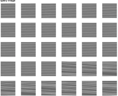
Figure 1 gives a retrieval result from the texture image database. All the 20 simi- lar textures in the database are retrieved in the first 20 images, and the remaining ones are also relevant. Figure 2 shows a retrieval result from a real world image database. As can be seen, most of the retrieved images are images with similar textu- res and colours to that in the query image. It shows us that the proposed technique works well for retrieval of images with homogeneous colour and texture overall.

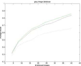
Figures 3 and 4 displays the comparison of the average recalls of the query images taken from texture image database and real world image database respecti- vely, the recall for which is defined as:

images relevant of

number

retrieved images

relevant of

number recall=

5. Conclusion

In this paper we have used the nonlinear monomial kernel function to capture the local structures of image content to find out the colour features. Such a technique does not require any segmentation and therefore works fully automatically [9, 12].

We have also used the Gabor function by applying some of appropriate dilations and rotations to base the texture features of the image on.

The extracted texture and colour features are then used to measure the similariti- es between the query image and the image database by weighting these feature types according to needs or according to image type. The retrieval results have been shown and examined.

Figure 1: Image retrieval results from a texture image database

Figure 3: Comparison of the average recalls by using different features: a solid curve for the combination of colour and texture features, a dashed curve for texture

feature and a dotted curve for the colour feature

Figure 4: Comparison of the average recalls by using different features: a solid curve for the combination of colour and texture features, a dashed curve for texture

feature and a dotted curve for the colour feature

References

[1] H. Burkhardt and S. Siggelkow, “Invariant features in pattern recognition fun- damentals and applications. In I.Pitas and C. Kotropoulos, editors, Non- linear Model Based Image/Video Processing and Analysis, pages 269–

307. John Wiley & Sons, 2001.

[2] George M. Haley and B. S. Manjunath, “Rotation invariant texture classification using a complete space-frequency model,” IEEE transactions on Image Processing, vol. 8, no. 2, pp. 255–269, February 1999.

[3] B. S. Manjunath and W. Y. Ma. “Texture features for browsing and retrieval for large image data” IEEE Transactions on Pattern Analysis and Machine Intelligence, Vol. 18, NO. 8, August 1996, pp. 837–842.

[4] B. S. Manjunath, P. Wu, S. Newsam, H. D. Shin, “A texture descriptor for browsing and similarity retrieval” Signal Processing: Image Commu- nication, 2000.

[5] R. Manthalkar, P. K. Biswas, “Rotation invariant texture classification using Gabor wavelets” Asian Conference on Computer Vision, pp. 493–498, Jan. 23–25, 2002, Melbourne Australia.

[6] R. Manthalkar, P. K. Biswas, “Color Texture Segmentation using multichannel filtering” Conference on Digital Image Computing Techniques and App- lication, pp. 346–351, Jan 21–22, Melbourne, Australia, 2002.

[7] R. Manthalkar, P. K. Biswas, B. N. Chatterji, ”Rotation and scale invariant textu- re classification using Gabor wavelets“ second international workshop on texture analysis and synthesis, 2002 Copenhagen.

[8] H. Schulz-Mirbach, “Invariant features for gray scale images” In G. Sagerer, S.

Posch, and F. Kummert, editors, 17. DAGM-Symposium, pages 1–14, Bielefeld, Germany, September 1995.

[9] S. Siggelkow and H. Burkhardt, “Image retrieval based on colour and nonlinear texture invariants” In S. Marshall, N. Harvey, and D. Shah, editors, Pro- cessings of the Noblesse Workshop on Non-Linear Model Based Image Analysis, pages 217–224, Glasgow, United Kingdom, July 1998.

[10] S. Siggelkow and H. Burkhardt, “Image retrieval based on local invariant featu- res” In IASTED International Conference on Signal and Image Proces- sing (SIP), pages 369–373, Las Vegas, NV, October 1998.

[11] S. Siggelkow, M. Schael, and H. Burkhardt “SIMBA- Search IMages By Appe- rance” In the B. Radig and S. Florczyk, editors, Pattern Recognition, DAGM, LNCS 2191, pages 9–16, München, Germany, September 2001.

[12] Sven Siggelkow. “Feature Histograms for Content-based Image Retrieval”

Ph.D thesis, Albert-Ludwigs-Universität Freiburg, Germany, 2002.