Detection of physical activity using machine learning methods
Lehel D´enes-Fazakas, L´aszl´o Szil´agyi, Jelena Tasic, Levente Kov´acs, Gy¨orgy Eigner Physiological Controls Research Center
Obuda University, Budapest, Hungary´
{denes-fazakas.lehel, szilagyi.laszlo}@nik.uni-obuda.hu,{jelena.tasic, kovacs, eigner.gyorgy}@uni-obuda.hu
Abstract—In the case of diabetes mellitus physical activity does have a high effect on the glycemic state of the patients.
This is especially regarding the patients with Type 1 diabetes mellitus, who need external insulin administration in their daily life. Nevertheless, physical activity – as one source of stress – is underrepresented in the decisions of patients and medical staff and in the decisions of the available automated glucose regulatory devices. The goal of the study was to build up a simulation framework for data generation and to assess which machine learning solution can be the most accurate in the identification of physical activity.
Index Terms—Machine Learning, Diabetes Mellitus, Physical Activity
I. INTRODUCTION
Diabetes mellitus (DM) is a chronic metabolic disease affecting millions of people worldwide. DM is connected to the insulin hormone. Insulin is the key protein which facilitates the entering of glucose molecules from blood plasma into several types of body cells. Hence, the blood glucose level decreases while the cells are able to use glucose as source of energy. In case of Type 1 DM (T1DM) the body is not able to produce insulin internally and the patients have to have external insulin administration. In case of Type 2 (T2DM) the body produces insulin, but often the effect of the hormone is not sufficient in terms of decreasing the blood glucose level [1].
One of the key components of the treatment for diabetics with T1DM is doing physical activity on a daily regimen which completes the external insulin administration and diabetic diet [2]. The stress caused by physical activity opens specific non- insulin dependent pathways in the cell-wall through which glucose is able to enter into the cells [3]. Thus, planned physical activity – beside its many positive effects – can help to regulate the blood glucose level and to increase the activity and effectiveness of the metabolic system. Due to this, the amount of externally administered insulin can be decreased if the physical activity is the organic part of the treatment [4].
This project has received funding from the European Research Council (ERC) under the European Union’s Horizon 2020 research and innovation programme (grant agreement No 679681). Project no. 2019-1.3.1-KK-2019- 00007 has been implemented with the support provided from the National Research, Development and Innovation Fund of Hungary, financed under the 2019-1.3.1-KK funding scheme. L. Szil´agyi is J´anos Bolyai Research Fellow of the Hungarian Academy of Sciences. L. D´enes-Fazakas was supported by the ´UNKP-20-2 New National Excellence Program of the Ministry for Innovation and Technology.
Nevertheless, not scheduled physical activity can be dan- gerous as well. If it is not considered by the diabetic patient during the calculation of necessary insulin amount, it can lead to overdosing of insulin which may lead to hypoglycemia [5].
Hypoglycemia is a dangerous condition for healthy people and even more risky for diabetics. The long-term hypoglycemic condition may cause cetoacidic conditions and lead to even coma or death over time. Thus, there is unquestionable need to consider the effect of physical activity in the daily life and especially if the treatment is semi-automatic, for example in case of insulin pump usage [6]. In the latter situation, the regulatory algorithms ought to take the scheduled and not scheduled physical activity into account. It is generally known that the physical activity causes the drop of the blood glucose level and increase of metabolic activity, with a certain time delay [7]. Namely, after the recognition of some sort of sports we still have time to intervene in to changing glycemic state.
Still, after the recognition of the activity the algorithms should be prepared for the appearance of the already mentioned consequences. This is one of the biggest unsolved challenge in the research community, namely, to find ways which are satisfyingly capable to recognize and consider the unscheduled physical activity.
The capability of machine learning based models to recog- nize patterns is not questionable and it has proven in many applications related to biomedical engineering [8]–[11]. In case of diabetes treatment their also proven their usefulness [12]–[15].
In this study, we aimed to develop a machine learning application which is able to recognize physical activity using only available information about the patient. We did not categorize the type of the activity, only the recognition of its presence was the goal, however. Due to the lack of massive patient data we developed a platform by using the extended Jacobs T1DM simulator [16] for massive data generation. Our goal was to make our solution as realistic as possible in this proof-of-concept phase in order to be easily implementable and testable in case of real patient data.
The paper is structured as follows. First, we introduce the data generation platform, the determining properties of the generated data and the selected features. After, we detail the applied machine learning resources and methods. That comes the introduction and interpretation of our results which is followed by our conclusions and the directions of our future
work.
II. MATERIALS AND METHODS
A. Applied dataset
The primary goal of the study was to identify what machine learning algorithms are the most beneficial to be used for the detection of physical activity using only blood glucose measurements. In this study, we apply synthetic data gener- ated by an extended version of the Jacobs T1DM simulator [17]. The simulator employs the Cambridge-model, however, it contains embedded physical activity submodel, which is an extension compared to the one presented in [18]. We applied the single hormone virtual patient population, where the simulator expects the insulin as control input only. The simulator provides 20 virtual patients with T1DM identified and validated based on a 3.5-day outpatient Artificial Pancreas (AP) study [17]. The simulator is open source, originally pub- lished on Github (https://github.com/petejacobs/T1D VPP). In order to make the data generation part more realistic, we completed the simulator with Continuous Glucose Monitoring System (CGMS) model from [19].
The simulator is easy to parametrize with respect to carbo- hydrate (CHO) and insulin intake. We applied the following regimens by using randomization regarding time instances and amounts of CHO intake:
• The times of meal consumption randomly varied between -30 minutes and +90 minutes with respect to prescribed times. The default time instances in the simulator were:
breakfast at 6 am, lunch at 12 pm and dinner at 6 pm.
• The amount of breakfast was set 35 ±10 [g].
• The amount at lunch varied between 79 ±10 [g]
• The amount at dinner varied between 117±10 [g].
• The duration of physical activity varied between 30 minutes to 90 minutes.
• The blood glucose level at the beginning of the day varied between 160 ±20 [mg/dL].
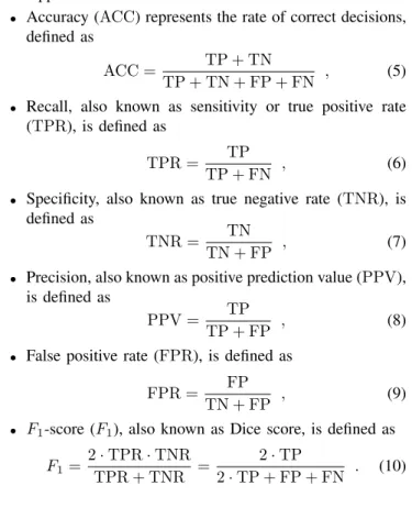
0 200 400 600 800 1000 1200 1400
0 100 200 300
0 200 400 600 800 1000 1200 1400
0 100 200 300
Fig. 1. Jacobs simulator model output indicating the physical activity with the red section on figure, without CGMS (top) and with CGMS (bottom)
The application of the CGMS model modifies the ”pure”
BG output value of the simulator - an example is given in Fig 1. We applied a realistic sampling time, namely, the blood glucose level was measured (simulated) by the CGM sensor every five minutes.
The synthetic data generation process were the following.
We have randomly selected 13 virtual patients from the available 20. During the data generation we did not change the parameters of the selected virtual patients.
For each patient, the simulation covered 640 days, not as a single very long simulation, but each day separately as a 24- hour simulation. Every day contained 288 sample points. We used a sliding window of 15 sample points to extract features.
Samples within the sliding window were indexed from 0 to 14. Thus we extracted 274 data rows per day. Each sliding window was divided into three smaller inclusive windows of five consecutive sample in each, having indexes 0 to 4, 5 to 9, and 10 to 14, respectively. From each sliding window we extracted 32 features. The ground truth of the dataset are listed in the following:
• The patient’s body weightw;
• End-to-end blood glucose level changeddefined as
d=bg(14)−bg(0) (1)
• The blood glucose level variation between consecutive sampled points, or in other words the first order differ- ences of blood glucose levels, defined as
dp(i) =bg(i+ 1)−bg(i) (2) for anyi= 0. . .13;
• End-to-end blood glucose level change in all inclusive sliding windows, defined as
dpp(i) =bg(5i+ 4)−bg(5i) (3) for anyi= 0. . .2;
• Second order changes of the blood glucose level, com- puted from 3 consecutive samples with the formula
ap(i) = dp(i+ 1)−dp(i)
= bg(i+ 2)−2×bg(i+ 1) +bg(i) (4) for anyi= 0. . .12;
• The decisiondc, which is used as ground truth throughout this study.
The whole data set contains 2,279,680 entities. 95% of these represent measurements with no activity (0) and 5% with activity (1). Because of this strong imbalance we can say this is a so-called anomaly detection problem in machine learning.
B. Outcome of the prediction
The goal of this study is to evaluate the accuracy and effectiveness of various machine learning algorithms, when they are applied to predict the physical activity of patients.
The outcome if the classification for each feature vector is binary, with the following two possibilities:
• 0 – No physical activity is currently performed by the patient.
• 1 – Physical activity is currently performed by the patient.
Some of the machine learning models (e.g. multi-layer perceptrons) involved in this study to predict the probability of physical activity (p∈[0,1]). In these cases a threshold is applied to the predicted probability, so that it can be interpreted in binary mode. Other models (e.g. decision tree) provide binary output directly. Such models do not need threshold, as their output is either 0 or 1.
C. Tested machnie learning models
This study involves eight different machine learning algo- rithms, some of them in multiple versions due to their param- eter settings, totally resulting in 13 models. These models and their descriptions, together with their unique ID are presented below.
• Logistic Regression[20], with maximum 1000 iterations, and L2-type penalty (LogReg);
• AdaBoost Classifier (Ada) [21] with maximum 50 trees;
• DecisionTree Classifier (DecTree) [22], [23] with unlim- ited tree depth and all decisions allowed to use any one of the features;
• Gaussian Naive Bayes (Gauss) [24];
• K-Nearest Neighbors Classifier (KNN) [25] using k−d tree implementation [26] and k= 5;
• Support Vector Machines [27] with 1000 iterations in five kernel variants: radial basis function kernel (SVM1), sigmoid kernel (SVM2), 3rd degree polynomial kernel (SVM3), 5th degree polynomial kernel (SMV4) and 10th degree polynomial kernel (SVM5);
• Random Forest [28], [29] with 100 trees (RF);
• Multi-Layer Perceptron Networks [30] with four hidden layers of sizes 100, 150, 100, and 50, respectively, maximum 1000 iterations, and three variants of activation functions: logistic (MLP1), ReLU (MLP2), and tanh (MLP3).
To implement these classification models, we used Python v2.7 programming language [31] and the Scikit package [32].
The total amount of available data was split into two sets, as follows: 75% of the feature vectors were randomly selected into the train data set, while the remaining 25% were assigned as evaluation (test) data. Feature vectors in the train data set were shuffled, so that two consecutive vectors are not likely to come from the same patient and simulation day.
For those classification algorithm, which are able to predict probabilities, the best threshold was established at the end of the training. The trained classifiers were applied to predict the presence or absence of physical activity for all feature vectors of the test data set. Statistical benchmarks, those presented in the next subsection, were established for each algorithm.
Further on, the ROC curve were drawn and the AUC values computed to evaluate the overall accuracy of the algorithms.
D. Performance evaluation
The performance evaluation of each model relies on the count of true positives (TP), true negatives (TN), false pos- itives (FP) and false negatives (FN). The following metrics were applied:
• Accuracy (ACC) represents the rate of correct decisions, defined as
ACC = TP + TN
TP + TN + FP + FN , (5)
• Recall, also known as sensitivity or true positive rate (TPR), is defined as
TPR = TP
TP + FN , (6)
• Specificity, also known as true negative rate (TNR), is defined as
TNR = TN
TN + FP , (7)
• Precision, also known as positive prediction value (PPV), is defined as
PPV = TP
TP + FP , (8)
• False positive rate (FPR), is defined as FPR = FP
TN + FP , (9)
• F1-score (F1), also known as Dice score, is defined as F1= 2·TPR·TNR
TPR + TNR = 2·TP
2·TP + FP + FN . (10)
III. RESULTS AND DISCUSSION
Table I presents the confusion matrix for all tested classi- fication models. Values presented in this table are normalized in each row. The classification can be called successful if the rate of both true positives and true negatives are high, typically above 0.8. Only the RF model achieved higher rate than 0.9 of both TP and TN, while KNN, AdaBoost, Decision Tree and all tested multi-layer perceptron models scored at both normalized indicators above 0.8. The three SVM models that used polynomial kernel apparently predicted the opposite.
Figure 2 presents the ROC curves of all classification models, while Figure 3 indicates the Area Under Curve (AUC) metric values, all values except those below 0.75. These two figures suggest that the Random Forest model performed the best, having AUC value of 0.98. However, knowing that an AUC above 0.8 can be considered as an excellent classification [33], KNN and all three MLP models, AdaBoost, and Decision Tree also produced acceptable classification.
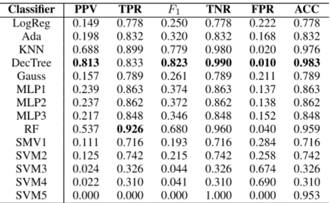
Table II presents the accuracy indicator metrics values for all tested classification models, highlighting the best value in each column. The better the classification the higher the indicator value in all cases except FPR. Although SVM5 apparently achieved perfect TNR and FPR, it cannot be highlighted as best achieved value because it predicted negative for every
TABLE I
NORMALIZED CONFUSION MATRIX OBTAINED BY THE USE OF VARIOUS CLASSIFICATION METHODS
Predicted value
0 1
Truevalue
0
LogReg : 0.779 LogReg : 0.221
Ada : 0.833 Ada : 0.167
KNN : 0.980 KNN : 0.020
DecTree : 0.991 DecTree : 0.009
Gauss : 0.789 Gauss : 0.211
SVM1 : 0.717 SVM1 : 0.283
SVM2 : 0.743 SVM2 : 0.257
SVM3 : 0.327 SVM3 : 0.673
SVM4 : 0.311 SVM4 : 0.689
SVM5 : 1.000 SVM5 : 0.000
RF : 0.961 RF : 0.039
MLP1 : 0.864 MLP1 : 0.136
MLP2 : 0.863 MLP2 : 0.137
MLP3 : 0.848 MLP3 : 0.152
1
LogReg : 0.221 LogReg : 0.779
Ada : 0.167 Ada : 0.833
KNN : 0.101 KNN : 0.898
DecTree : 0.166 DecTree : 0.834
Gauss : 0.211 Gauss : 0.789
SVM1 : 0.284 SVM1 : 0.716
SVM2 : 0.257 SVM2 : 0.743
SVM3 : 0.673 SVM3 : 0.327
SVM4 : 0.689 SVM4 : 0.311
SVM5 : 1.000 SVM5 : 0.000
RF : 0.073 RF : 0.927
MLP1 : 0.136 MLP1 : 0.864
MLP2 : 0.137 MLP2 : 0.863
MLP3 : 0.152 MLP3 : 0.848
Fig. 2. ROC curve of models
tested feature vector. According to the results, DecTree has the most highlighted best values, while Random Forest has the highest Recall value. KNN is the model that also has acceptable values at all indicators. All others predicted too many false positives, which is best visible in the column of PPV values that penalizes false positives. Classifiers with finest outcome are those which have high values in both recall
Fig. 3. AUC values obtained by various classification models
TABLE II
OBTAINED ACCURACY INDICATOR METRICS VALUES FOR ALL CLASSIFICATION MODELS
Classifier PPV TPR F1 TNR FPR ACC
LogReg 0.149 0.778 0.250 0.778 0.222 0.778 Ada 0.198 0.832 0.320 0.832 0.168 0.832 KNN 0.688 0.899 0.779 0.980 0.020 0.976 DecTree 0.813 0.833 0.823 0.990 0.010 0.983 Gauss 0.157 0.789 0.261 0.789 0.211 0.789 MLP1 0.239 0.863 0.374 0.863 0.137 0.863 MLP2 0.237 0.862 0.372 0.862 0.138 0.862 MLP3 0.217 0.848 0.346 0.848 0.152 0.848 RF 0.537 0.926 0.680 0.960 0.040 0.959 SMV1 0.111 0.716 0.193 0.716 0.284 0.716 SVM2 0.125 0.742 0.215 0.742 0.258 0.742 SVM3 0.024 0.326 0.044 0.326 0.674 0.326 SVM4 0.022 0.310 0.041 0.310 0.690 0.310 SVM5 0.000 0.000 0.000 1.000 0.000 0.953
(TPR) and positive PPV, namely, the Decision Tree, KNN, and Random Forest. The same benchmark is indicated by the F1-score column, which equally penalizes false positives and false negatives, and gives the highest values to the same three classification models.
To establish a unique ranking of the employed classification models, it is necessary to inspect those benchmark values, which penalize both kinds of mistaken decisions, namely false positives and false negatives. Recall (TPR) and speci- ficity (TNR) together are able to characterize the accuracy of the classification performance, while the F1-score, which is the harmonic mean of TPR and TNR, unifies these two benchmarks into a single score. Having a high recall value is necessary for an accurate classification, because the rare positive cases need to be identified with a high probability.
In case of a serious imbalance between actual positive and negative cases, it is good to have a TNR value very close to 1 (e.g. like DecTree and KNN in Table II), otherwise the number of false positives is too high. The high number of false positives in Table II is best reflected by the PPV benchmarks, which penalize true positives but discriminates more strongly than the TNR value. The last column of Table II reflects the rate of correct decisions also called overall accuracy (ACC), which in case of such imbalanced data (approx. 95%
negatives and 5% positives), may lead to anomaly or mistaken conclusions. In this order, the ACC value is quite high for the
SVM5 classifier, which in fact predicts negative for all test data.
Based on the above criteria, we can assert that the three best classifiers for the given problem are the Decision Tree, K-Nearest Neighbors andRandom Forest, which scored high at those benchmarks that penalize all mistaken decisions.
IV. CONCLUSIONS AND FUTURE WORK
This paper introduced a machine learning based framework for the detection of physical activity, using features extracted from blood glucose samples taken at five minutes intervals.
Several classification models were involved in the study using various parameter settings. The statistical evaluation revealed that three of the tested models, namely the KNN, the Decision Tree and the Random Forest are the most suitable for the given problem, while several others can be made suitable but they need an extra mechanism to avoid the most part of the false positives. This sort of difficulty is quite common in classification problems where the amount of positives and negatives is imbalanced.
Future work will include collecting data from real patients and using them to validate classification algorithms that would detect physical activity. Further on, the developed model will be integrated into Apple watch and android mobile application, which will receive data from sensors, transmit the data to a database, and will make predictions, having the possibility to notify the doctor if the patient seems to be in bad condition.
REFERENCES
[1] R. I. Holt, C. Cockram, A. Flyvbjerg, and B. J. Goldstein,Textbook of diabetes. Chichester, UK: John Wiley & Sons, 2017.
[2] S. R. Bird and J. A. Hawley, “Update on the effects of physical activity on insulin sensitivity in humans,”BMJ Open Sport Exerc Med, vol. 2, no. 1, p. e000143, 2017.
[3] C. Zhao, C. F. Yang, S. Tang, C. Wai, Y. Zhang, M. P. Portillo, P. Paoli, Y. J. Wu, W. S. Cheang, B. Liu, C. Carp´en´e, J. B. Xiao, and H. Cao,
“Regulation of glucose metabolism by bioactive phytochemicals for the management of type 2 diabetes mellitus,” Critical Reviews in Food Science and Nutrition, vol. 59, no. 6, pp. 830–847, 2019.
[4] S. R. Colberg, R. J. Sigal, J. E. Yardley, M. C. Riddell, D. W. Dunstan, P. C. Dempsey, E. S. Horton, K. Castorino, and D. F. Tate, “Physical activity/exercise and diabetes: A position statement of the american diabetes association,”Diabetes Care, vol. 39, no. 11, pp. 2065–2079, 2016.
[5] P. Martyn-Nemeth, L. Quinn, S. Penckofer, C. Park, V. Hofer, and L. Burke, “Fear of hypoglycemia: Influence on glycemic variability and self-management behavior in young adults with type 1 diabetes,”Journal of Diabetes and its Complications, vol. 31, no. 4, pp. 735–741, 2017.
[6] N. Jeandidier, J. P. Riveline, N. Tubiana-Rufi, A. Vambergue, B. Catargi, V. Melki, G. Charpentier, and B. Guerci, “Treatment of diabetes mel- litus using an external insulin pump in clinical practice,”Diabetes &
Metabolism, vol. 34, no. 4, pp. 425–438, 2008.
[7] P. O. Adams, “The impact of brief high-intensity exercise on blood glucose levels,”Diabetes Metab. Syndr. Obes., vol. 6, pp. 113–122, 2013.
[8] L. Liang, F. W. Kong, C. Martin, T. Pham, Q. Wang, J. Duncan, and W. Sun, “Machine learning–based 3-d geometry reconstruction and modeling of aortic valve deformation using 3-d computed tomography images,”Int J Numer Meth Biomed Engng, vol. 33, p. e2827, 2017.
[9] S. M. Lundberg, B. Nair, M. S. Vavilala, M. Horibe, M. J. Eisses, T. Adams, D. E. Liston, D. K.-W. Low, S.-F. Newman, J. Kim, and S.-I. Lee, “Explainable machine-learning predictions for the prevention of hypoxaemia during surgery,”Int J Numer Meth Biomed Engng, vol. 2, no. 10, pp. 749–760, 2018.
[10] S. Ostrogonac, E. Pakoci, M. Seˇcujski, and D. Miˇskovi´c, “Morphology- based vs unsupervised word clustering for training language models for serbian,” Acta Polytechnica Hungarica: Journal of Applied Sciences, 2019.
[11] K. Machov´a, M. Mach, and M. Hreˇskov´a, “Classification of special web reviewers based on various regression methods,”Acta Polytechnica Hungarica, vol. 17, no. 3, 2020.
[12] A. Hayeri, “Predicting future glucose fluctuations using machine learn- ing and wearable sensor data,”Diabetes, vol. 67, no. Suppl. 1, p. A193, 2018.
[13] E. Daskalaki, P. Diem, and S. G. Mougiakakou, “Model-free machine learning in biomedicine: Feasibility study in type 1 diabetes,”PloS one, vol. 11, no. 7, p. e0158722, 2016.
[14] A. Z. Woldaregay, E. ˚Arsand, T. Botsis, D. Albers, L. Mamykina, and G. Hartvigsen, “Data-driven blood glucose pattern classification and anomalies detection: Machine-learning applications in type 1 diabetes,”
Journal of medical Internet research, vol. 21, no. 5, p. e11030, 2019.
[15] I. Contreras and J. Vehi, “Artificial intelligence for diabetes management and decision support: literature review,” Journal of Medical Internet Research, vol. 20, no. 5, p. e10775, 2018.
[16] P. G. Jacobs, J. El Youssef, J. R. Castle, J. R. Engle, D. L. Branigan, P. Johnson, R. Massoud, A. Kamath, and W. K. Ward, “Development of a fully automated closed loop artificial pancreas control system with dual pump delivery of insulin and glucagon,” in2011 Annual International Conference of IEEE EMBS. IEEE, 2011, pp. 397–400.
[17] N. Resalat, J. El Youssef, N. Tyler, J. Castle, and P. G. Jacobs, “A statistical virtual patient population for the glucoregulatory system in type 1 diabetes with integrated exercise model,”PloS One, vol. 14, no. 7, 2019.
[18] M. M. N. Nærum, “Model predictive control for insulin administration in people with type 1 diabetes,” BSc Thesis, Kongens Lyngby, 2010.
[19] D. Boiroux and J. B. Jørgensen, “A nonlinear model predictive control strategy for glucose control in people with type 1 diabetes,” IFAC- PapersOnline, vol. 51-27, pp. 192–197, 2018.
[20] D. R. Cox, “The regression analysis of binary sequences (with discus- sion),”J R Stat Soc B, vol. 20, no. 2, pp. 215–242, 1958.
[21] Y. Freund and R. E. Schapire, “Experiments with a new boosting algorithm,” in 13th International Conference on Machine Learning, 1996, pp. 148–157.
[22] S. B. Akers, “Binary decision diagrams,”IEEE Transactions on Com- puters, vol. C-27, no. 6, pp. 509–516, 1978.
[23] L. Szil´agyi, D. Icl˘anzan, Z. Kap´as, Z. Szab´o, Gy˝orfi, and L. Lefkovits,
“Low and high grade glioma segmentation in multispectral brain mri data,” Acta Universitatis Sapientiae – Informatica, vol. 10, no. 1, pp.
110–132, 2018.
[24] C. K. Chow, “An optimum character recognition system using decision functions,” IRE Transactions on Computers, vol. EC-6, pp. 247–254, 1957.
[25] T. M. Cover and P. E. Hart, “Nearest neighbor pattern classification,”
IEEE Transactions on Information Theory, vol. IT-13, pp. 21–27, 1967.
[26] J. L. Bentley, “Multidimensional binary search trees used for associative searching,”Communications of the ACM, vol. 18, no. 9, pp. 509–517, 1975.
[27] C. Cortes and V. Vapnik, “Support-vector networks,”Machine Learning, vol. 20, pp. 273–297, 1995.
[28] L. Breiman, “Random forests,”Machine Learning, vol. 45, no. 1, pp.
5–32, 2001.
[29] E. Alfaro-Cort´es, J.-L. Alfaro-Navarro, M. G´amez, and N. Garc´ıa,
“Using random forest to interpret out-of-control signals,”Acta Polytech.
Hung., vol. 17, no. 6, pp. 115–130, 2020.
[30] D. E. Rumelhart, G. E. Hinton, and R. J. Williams, “Learning repre- sentations by back-propagating errors,”Nature, vol. 323, no. 6088, pp.
533–536, 1986.
[31] Python Language Reference, Python Software Foundation, Version 2.7, 2020, available at http://www.python.org.
[32] F. Pedregosa, G. Varoquaux, A. Gramfort, V. Michel, B. Thirion, O. Grisel, M. Blondel, P. Prettenhofer, R. Weiss, V. Dubourg, J. Vander- plas, A. Passos, D. Cournapeau, M. Brucher, M. Perrot, and E. Duch- esnay, “Scikit-learn: Machine learning in Python,”Journal of Machine Learning Research, vol. 12, pp. 2825–2830, 2011.
[33] O. P. Trifonova, P. G. Lokhov, and A. I. Archakov, “Metabolic profiling of human blood,”Biochem. Moscow Suppl. Ser. B, vol. 7, pp. 179–186, 2013.