2. SIR model

(1)

Replacing the SIR epidemic model with a neural network and training it further to

increase prediction accuracy ^∗†

Gergő Bogacsovics, András Hajdu, Róbert Lakatos, Marcell Beregi-Kovács, Attila Tiba, Henrietta Tomán

University of Debrecen bogacsovics.gergo@inf.unideb.hu

hajdu.andras@inf.unideb.hu robert.lakatos@it.unideb.hu beregi.kovacs.marcell@science.unideb.hu

tiba.attila@inf.unideb.hu toman.henrietta@inf.unideb.hu

Submitted: December 21, 2020 Accepted: February 17, 2021 Published online: May 18, 2021

Abstract

Researchers often use theoretical models which provide a relatively simple, yet concise and effective way of modelling various phenomena. However, it is a well-known fact that the more complex the model, the more complex the mathematical description is. For this reason, theoretical models generally avoid large complexity and aim for the simplest possible definition, which al- though makes models mathematically more manageable, in practice it also often leads to sub-optimal performance. Furthermore, the data collected during the observations usually contain confounding factors, for which a simple theoretical model can not be prepared. Overall, mathematical models are usually too rigid and sophisticated, and therefore cannot really deal with

∗The research was partly supported by the 1st Cloud Funding for Research Open Call of Open Clouds for Research Environments (OCRE), by the ÚNKP-20-4-I New National Excellence Program of the Ministry for Innovation and Technology from the Source of the National Research, Development and Innovation Fund and by the project EFOP-3.6.2-16-2017-00015 supported by the European Union, co-financed by the European Social Fund.

†Equal contribution.

doi: https://doi.org/10.33039/ami.2021.02.003 url: https://ami.uni-eszterhazy.hu

73

(2)

sudden changes in the environment. The application of artificial intelligence, however, provides a good opportunity to develop complex models that can combine the basic capabilities of the theoretical models with the ability to learn more complex relationships. It has been shown [16] that with neural networks, we can build such models that can approximate mathematical functions. Trained artificial neural networks are thus able to behave like theoretical models developed for different fields, while still retaining their overall flexibility, which guarantees an overall better performance in a complex real- world environment.

The aim of our study is to show our notion that we can create an architecture using neural networks, which is able to approximate a given theoretical model, and then further improve it with the help of real data to suit the real world and its various aspects better. In order to validate the functionality of the architecture developed by us, we have selected a simple theoretical model, namely the Kermack-McKendrick one [4] as the base of our research. This is an SIR [2] model, which is a relatively simple compartmental epidemic model, based on differential equations that can be used well for infections that spread very similarly to influenza or COVID. However, on one hand, the SIR model relies too heavily on its parameters, with slight changes in them leading to drastic overall changes of the S, I and R curves, and on the other hand, the simplicity of the SIR model distorts its accuracy in many cases. In our paper, by using the SIR model, we will show that the architecture described above can be a valid approach to modeling the spread of a given disease (such as influenza or COVID-19). To this end, we detail the accuracy of our models with different settings and configurations and show that it performs better than both a simple mathematical model and a plain neural network with randomly initialized weights.

Keywords: Deep learning, neural networks, mathematical models, approximation, parameter optimization, SIR model

1. Introduction

The appearance of COVID-19 made 2020 a very memorable year. It affected nearly all of the countries in the world, leading to quarantines and regulations that the people of the 21st century have never experienced before, while also delivering a heavy blow to the global economy, thus resulting in people losing their jobs. Not only that, the number of people dying due to this disease has also reached heights that was previously unimaginable. Therefore, it goes without saying that examining and researching this disease is of utmost importance to better understand its mechanics and driving forces.

Pure mathematical models have been very frequently used for modeling the spread of diseases like influenza [9, 12], measles [17] and so on. This is mainly due to their simplicity and mathematical foundations, which guarantees a compact, yet concise, effective and simple-to-explain model. However, the accuracy of pure mathematical models, such as SIR [4], SIS [1], SEIR [7], SEIRS [5], is often sub- optimal, which is precisely due to this simplicity. The prediction curve of an SIR

(3)

model for example is a simple bell-shaped curve, which means that a single SIR model cannot perform well when examining diseases like COVID-19, that have multiple waves. One possible solution to that problem is to fit multiple SIR models to the data. However, that is not optimal either, because we need to manually group the data into segments first, and then fit the SIR models to these groups.

Selecting these groups manually however is not a trivial task, as the grouping affects the fitting phase, meaning that a bad grouping results in worse fitting and therefore yields worse results. This can easily be solved by using neural networks, since they can generalize well and achieve state-of-the-art accuracy in just about every field of science. One problem with using pure neural network models is the lack of quality data. For example, even though almost a year has passed since the initial outbreak of COVID-19, there are only around 200-300 data points per country to learn from, since data was usually gathered on a daily basis. Another problem is that COVID data often have huge amounts of noise due to how the recording of the daily cases took place and other factors. These can however heavily affect both the training phase (since the network will be much likely have a higher bias) and the performance of the network (since it will not be able to generalize well).

The goal of our research is to show that mathematical models, which are used frequently in investigating disease spread, epidemiology and even COVID-19 [15], can be applied to the training of neural network models as a pretraining step, resulting in a more accurate model. In our paper we show that if we train a neural network first on an SIR model, then train it further on real data, this method outperforms not only the original mathematical model, but also a neural network trained only on real data. This is because this way the neural network not only has access to more data (SIR data and real data), but the initial training phase (approximating the SIR model) is mathematically well-defined and the data points are not noisy, unlike the real data. This way, the neural network will have a solid set of weights before being trained on real data, that are roughly equivalent to a mathematical SIR model, making the second part of the training much smoother and easier. We also show that a neural network trained in this way can easily overcome the biggest obstacle of SIR models described above, which is not being able to forecast multiple waves by making predictions regarding the second wave of COVID-19 by training the models only on the first wave and evaluated on the second wave.

In this paper we outline a simple architectural solution regarding the model by using a simple neural network as the base. The data that the models operate on contain the daily number of newly infected patients and all the models were trained on data constructed from the original data by using a sliding window approach.

This means that the models receive the number of infected people in the last𝑡days, and predict that for the next 𝑇 days. In other words, inputs were of length𝑡, and the outputs were of length𝑇, where each element was the number of newly infected people on a given day. We have used different values for 𝑡 and 𝑇, respectively to achieve even better performances. Since due to the nature of the model, there will be multiple predictions for a given day, we also outline an aggregated solution

(4)

that combines the outputs of a single model for a given day by taking the mean of the predicted values. It is important to note that while in this paper we focus on deterministic models, due to its simple nature our proposed architecture can be used for stochastic models as well without any further restrictions.

The rest of the paper is organized as follows. In section 2 we present the SIR model and talk about its parameters and their effects on the performance of the model. In section 3 we briefly describe how the data used in the research was gathered. In section 4 we present our proposed two-step architecture and how it can be applied in practice. In section 5 we show how this architecture can be used on a simple and easier Influenza dataset, then in section 6 we show how these models achieve better results than normal neural networks whose weights have been initialized randomly for COVID-19 data. Finally, in the last section we summarize the results of our research.

2. SIR model

SIR is a general virus spread model that can be interpreted easily. The model can be described with an ordinary differential equation and has only a few parameters. Furthermore, in terms of behaviour it is a non-linear system. It is primarily recommended to be used for viruses where infected individuals cannot develop long-lasting immunity after recovery. This theoretical approach with regard to the spread of viruses was first described by William Ogilvy Kermack and Anderson Gray McKendrick and became generally known as the Kermack – McKendrick theory. We used this model in our research because currently, for both influenza and COVID-19, the scientific consensus is that, based on the behavioral characteristics of the virus, individuals cannot get sustained immunity after recovering.

The classic SIR model can be considered as a system of the following differential equations:

𝑑𝑆 𝑑𝑡 = 𝛽𝐼𝑆

𝑁 𝑑𝐼

𝑑𝑡 = 𝛽𝐼𝑆 𝑁 −𝛾𝐼 𝑑𝑅

𝑑𝑡 =𝛾𝐼 with the following notation of the parameters:

• 𝑆: Number of susceptible individuals.

• 𝐼: Number of infectious individuals.

• 𝑅: Number of recovered individuals.

• 𝑁: Total population.

• 𝑡: A given moment in time.

(5)

• 𝛽: Potential exposure rate per capita. Namely, it describes how many addi- tional individuals a particular infected can infect at a given point in time.

• 𝛾: Rate of recovery, which is practically the recovery/death rate and 1/𝛾 is the infectious period.

We only need to study the equations for two of the three variables𝑆,𝐼and𝑅, because

𝑑𝑆 𝑑𝑡 +𝑑𝐼

𝑑𝑡 +𝑑𝑅 𝑑𝑡 = 0, which follows from the fact that

𝑆(𝑡) +𝐼(𝑡) +𝑅(𝑡) =𝑁.

For the basic reproduction number, we have 𝑅(0) = 𝛽

𝛾.

3. Countries and data

For our research, we used infection data regarding influenza and COVID-19 viruses.

For influenza-related studies, we examined the data published by the World Health Organization (WHO) between 2018 and 2019. WHO makes the data FluNet¹[14]

available by year and every record in the dataset consists of weekly values.

For COVID-19, we were working on data for new cases published by the Johns Hopkins Coronavirus Research Center [3]. Johns Hopkins University actualizes the data every day and makes it available on the open humanitarian data sharing platform (HDX). On the provided HDX platform, the start date of public dataset² [11] is 22 January, 2020.

Furthermore, for both COVID-19 and influenza we tested our proposed architecture on data for several different countries, like Austria, China, Croatia, Germany, Hungary, Japan, Romania. The full list of countries considered can be seen in the corresponding sections of the paper (Section 5 and 6). Our experimental results first focus on Hungary by comparing the Hungarian data with the ones of its neighbors. Then we extend our study to developed, leading countries providing presumably the most accurate data.

In case of the SIR model, one of the most important parameters is the population of the studied area. The knowledge of the population is essential for the SIR model because one of the starting conditions for calculating the theoretical model is the number of infectious individuals. Population data for the countries were collected from a public (total population) database³ [13] which is currently main- tained by the World Bank. In the analysis, we used the most recent and available population data for 2019 for both viruses.

1https://www.who.int/influenza/gisrs_laboratory/flunet/en/

2https://data.humdata.org/dataset/novel-coronavirus-2019-ncov-cases

3https://data.worldbank.org/indicator/SP.POP.TOTL?name_desc=false

(6)

4. Two-step architecture

In this section, we describe the mechanism of our proposed two-step architecture.

First, we detail how we used the SIR model and how we extracted the optimal 𝛾 and𝛽 parameters for the model. Then, we present how we applied this fitted SIR model for training a more robust neural network model.

4.1. Determining the optimal parameters

A properly parameterized SIR model already has an acceptable prediction capability by itself. So when we approximate a theoretical model with a neural network, primarily this capability of the theoretical model is needed to be learnt. Namely, we would like to keep all information in the machine-learned model that can be extracted from the theoretical model. Furthermore, with the neural network, we aim to further improve such parameterized SIR models that best describe the real data. Accordingly, the first step in creating our own models was to find the𝛾and𝛽 parameters that generate such theoretical models which fit the real data the best.

Figure 1. A slice from the big solution space (left) and a SIR curve fitted to the German data (right).

In the case of SIR, we have a non-linear least-squares minimization problem with a large solution space due to the peculiarities of the SIR model, as it can be seen on Figure 1. There are several methods for solving such problems, like gradient descent, Gauss-Newton algorithm, Levenberg-Marquardt algorithm [6, 8], or differential evolution [10]. In the experimental phase, we compared several solution methods (BFGS, Newton, brute force, etc.) out of which the Levenberg- Marquardt algorithm (LMA) and differential evolution algorithms (DEA) proved to be the most efficient ones. LMA is a fast and effective algorithm finding an ideal solution even if started from initial values relatively far from the optimum.

Because of this property, it is applicable to determine proper starting parameters and their associated parameter range. DEA is proved to be slower than LMA, but starting with the same initial parameters, it generally finds a better solution than LMA. Because of its construction, DEA works more efficiently in the case of large solution spaces, like those occurring in optimization of SIR models.

(7)

Overall, our experience shows that both methods are well applicable to the curve fitting problem and can be used to find the optimal SIR model fitting best to real data (see Figure 1). Levenberg-Marquardt algorithm is especially advantageous because of its speed and the differential evolution algorithm is effective in further refining the existing near-optimal parameters.

4.2. Approximation

For approximating the spread of infectious disease, we apply a two-step architecture. First, we fit a SIR model to the given data (e.g. by searching for the optimal 𝛽 and 𝛾 values). Then, we fit a neural network to the (infected) curve 𝐼 of this SIR model, following the mechanism (concentrating only on curve 𝐼) of most of the methods applied in this field. This approach, of course, led to shorter training times and easier convergence. After the neural network obtained a set of weights that was roughly equivalent to the given SIR model (the predictions were close to the curve 𝐼 of the SIR model), we decreased the learning rate and trained the neural network on real data. This step is applied to make sure that the weights of the neural network do not change substantially, which could have resulted in a model that no longer resembles the original SIR model. Another advantage of the decreased learning rate is that the impact of the noise present in real data can be reduced in this way.

Figure 2. The basic workflow of the two-step architecture.

This approach (see Figure 2) has quite a few benefits compared to training a neural network directly on real data. First of all, the amount of noise generated throughout the training phase is considerably reduced, thanks to the model being taught on a much smoother and mathematically well-defined function, which is the output of the SIR model. The shape of the infected curve (𝐼) for a given SIR model is bell-shaped, with no irregularities and noise, hence it is easier for neural networks to be trained on. Moreover, since the network has a solid set of weights after the first phase is finished and the learning rate is smaller during the second phase, the irregularities present in real data do not affect the training as much as they would normally. This fact, along with the ability of an SIR model to approximate the original data fairly well, leads to a more controlled training, during which the network can first extract meaningful information about the nature of the disease, and then it has access to a more irregular dataset for further training. Another huge advantage of this architecture is the increased amount of data available during the learning phase. It is beneficial when the available dataset contains only a handful of records (as in case of the Influenza dataset in our study). However, by pretraining on a mathematical model that behaves roughly the same, we can generate the necessary data points to obtain such a starting set of weights that only needs

(8)

to be further refined on real data, hence leading to a smoother and more controlled training process.

During the experiments, we used a simple dense network with three hidden layers of 20, 40, 20 neurons and ReLU activation function in each layer. We focused on this simpler architecture instead of using more sophisticated ones like RNNs, LSTMs or GRUs to show that the proposed architecture can be used for a variety of problems. This time, we made the model function similar to a simple RNN by feeding it data containing several timesteps as input but this is not required; the architecture itself can be used for non-time step series data as well. Additionally, for handling time series data, we have considered using a neural network that does not only receive the data for the previous day and predicts the next day, but receives a sequence of 𝑡 days as input, and makes predictions regarding a sequence of 𝑇 days. We hand-picked the potential values for 𝑡 and𝑇, respectively, according to recent public forecasts that focus on the recent past and near future and kept 𝑇 smaller than 𝑡, since predicting more days than what the network has information on would be impractical.

5. Influenza

To demonstrate the basic idea behind the architecture, we decided to start by showing how it can be used for known diseases, like Influenza. For these diseases, there are already some mathematically defined models, which are used heavily in practice due to their simplicity and good overall performances. Therefore, we will show how one such model, the SIR model performs on data for a few selected countries and how we can further improve the performance by using our proposed two-step architecture.

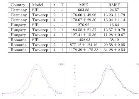
To measure the efficiency of these models, we used the available data of Ger- many, Hungary and Romania for the influenza season 2019 (starting from the winter of 2018 and ending in the spring of 2019). We chose these countries specifically from a bigger pool of countries by selecting those that had a data roughly resem- bling an SIR curve (see Figure 3). Our aim is to show that we can improve the overall performance of the original mathematical model even in cases where they perform relatively well.

Figure 3. A comparison between real influenza data and the fitted SIR curves for Germany, Hungary and Romania.

(9)

The dataset we used contained the weekly number of newly infected people for any given time step. Since the data was aggregated at a weekly level, we used the configuration 𝑡 ∈ {2,4}, 𝑇 = 1 for the neural network model. This way, it could process some relatively recent information (the last 2 or 4 weeks) without relying too much on older information (where 𝑡 > 4), while keeping the model relatively simple (𝑇 = 1) and suitable for showcasing the potential of the architecture.

The predictions were evaluated by calculating the mean square error (MSE) and root mean square error (RMSE) metrics. Furthermore, for every country and configuration, we trained five different neural networks to calculate the spread of the errors. Table 1 shows the summarized results of both the SIR and the two- step architecture considering a confidence level of 95% (𝑝 = 0.05, 𝑛 = 5, using 𝑡-statistics).

Table 1. The results of the SIR and the two-step architecture on the influenza dataset.

Country Model t T MSE RMSE

Germany SIR - - 603.88 24.57

Germany Two-step 2 1 176.66±49.96 13.23±1.79 Germany Two-step 4 1 170.67±29.50 13.04±1.14

Hungary SIR - - 276.92 16.64

Hungary Two-step 2 1 184.58±21.57 13.57±0.79 Hungary Two-step 4 1 127.41±15.36 11.28±0.67

Romania SIR - - 1452.93 38.12

Romania Two-step 2 1 877.12±124.16 29.58±2.05 Romania Two-step 4 1 1178.39±175.33 34.28±2.54

Figure 4. A comparison between the original SIR model (left) and one of the𝑡= 4, 𝑇 = 1models (right) for Germany.

It can be seen that by using our proposed two-step neural network architecture, we were able to drastically decrease the overall error in our predictions. The im- provements were the most drastic for the German and Romanian data, since while the SIR model fit relatively well to the real data, there were still a number of data points that were far away from the curves 𝐼 of the models (see Figure 4). This shows that using our proposed architecture can further increase the overall performance even in cases where the original mathematical model performs well and thus can be a plausible solution for tackling the spread of some diseases to achieve

(10)

state-of-the-art results. In the next section, we will show how this approach can be used for predicting the spread of COVID-19.

6. Covid-19

To fully demonstrate the capabilities of the proposed architecture, we ran some experiments on COVID-19 data. We think that choosing this disease can better showcase the performance and reliability of our architecture, since at the time of writing this paper there are no mathematical models that can perform really well on COVID-19 data. As outlined previously, there are several factors, such as the numerous waves, noise in the data, regulations that make predicting COVID-19 hard or impossible for a single simple mathematical model and our architecture aims to overcome these hardships. Moreover, these factors make training a neural network harder, too, since the noise present in the dataset may mislead the networks during the training phase.

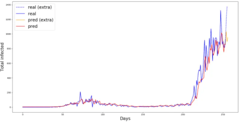
Figure 5. A model with the configuration 𝑡= 7, 𝑇 = 3 and its predictions (red & orange) for Hungary.

During the experiments, we used different values for 𝑇 and 𝑡, respectively to find out how many days’ worth of data can better describe the disease as well as to improve the overall performance. Namely, we used the configurations {(𝑡, 𝑇)|𝑡 ∈ {14,7,3}and𝑇 ∈ {7,3,1} and𝑇 < 𝑡}, since the available data was aggregated at a daily level. This way, we experimented with how many days the model should take into account when making predictions and find out whether increasing the size of the input resulted in any substantial performance gains. We also tried changing the output size to experiment with whether doing so could make the model more reliable by having it constantly focus on a series of next days. The dataset that we used contained the number of newly infected people for any given time step.

We found that using𝑡 >14 made the training of the model much harder and resulted in models that performed worse due to making the model more complex and it focuses too much on days too far away and therefore does not contribute to

(11)

the current number of infected people. For a similar reason, we observed that when 𝑇 was closer to𝑡, the overall performance plummeted, since the model simply did not have enough information to make accurate long-term predictions. Moreover, we found that when𝑇 >3, the quality of the predictions regarding the future started to deteriorate, suggesting that predictions with a larger output window size for the COVID-19 dataset are not yet feasible. Instead, we suggest that it is better to use smaller𝑇 values instead of trying to make long-term predictions (see Figure 5).

We trained all the models on the first wave of COVID-19 for any given country.

This means that we first fit a SIR model to the data of the first wave, then approx- imated the curve 𝐼with a neural network, then trained it further on the real data of the first wave. Then, we tested the models on the second wave of COVID-19 for the given country. To test the overall reliability and performance of our proposed architecture, we compared its results with a plain neural network that was not initialized with weights similar to an SIR model but simply trained on the available COVID-19 data. These plain neural networks were also trained in the exact same way: first fit to the first wave of the real data and then tested on the second wave.

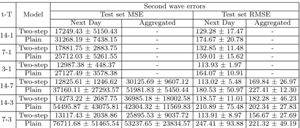
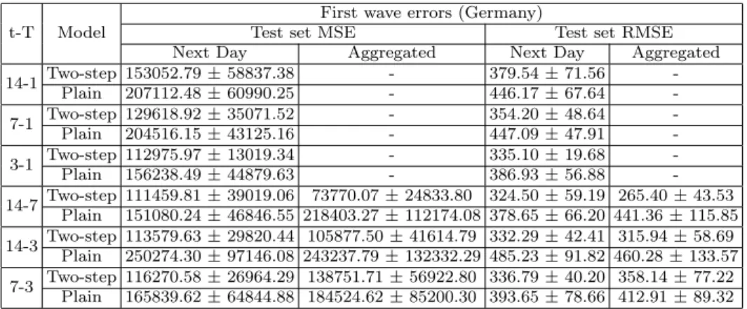
We repeated each experiment for a given(𝑡, 𝑇)pair a total of𝑛times to measure how the results fluctuated. During our research, we found the number 10 to be the best for this purpose: the samples gathered proved to be representative enough to reliably calculate the overall error while the time required to train the models was still manageable. Tables 2, 3, 4 and 5 show the summarized results of both the two-step architecture (denoted as “Two-step”) and the plain neural network models (denoted as “Plain”), calculated with a confidence level of 95% (𝑝= 0.05, 𝑛= 10, using t-statistics) for Hungary and Germany. We deliberately put more focus on these two countries since we wanted to examine how the spread of the disease can be modelled for Hungary and for a more developed country, like Germany. The results regarding the other countries can be found in Appendix, calculated with a confidence level of 95% but with a lower sample size of 3 (𝑝= 0.05, 𝑛= 3,using t-statistics).

It can easily be seen that the results of the proposed architecture are generally way better than that of a simple, randomly initialized neural network. It shows that having the model learn a less complex and mathematically better defined function that roughly resembles the target data may be a beneficial pre-training step and could yield potentially better results when trained further on real data compared to models that are trained only on the latter. Another important note is that the target mathematical function does not need to match precisely with the real data, as it was the case for our research regarding COVID-19: the only important part is that it should contain some key information (in this case the bell-shape curve hinting that the number of diseases should keep increasing until a certain point and then start decreasing from then on) that can provide a strong foundation for the network to build upon in the second phase of the training. This approach also makes it harder for the model to focus on dispensable features due to the first step containing the differential equations in its loss function. Another interesting point is that training the network on a SIR model for the first wave is proved to

(12)

Table 2. Hungary - first wave errors.

t-T Model First wave errors

Test set MSE Test set RMSE

Next Day Aggregated Next Day Aggregated

14-1 Two-step 86.84±20.39 - 9.21±1.05 -

Plain 271.51±52.64 - 16.35±1.54 -

7-1 Two-step 107.55±19.33 - 10.29±0.99 -

Plain 186.41±31.68 - 13.57±1.16 -

3-1 Two-step 98.51±11.96 - 9.89±0.59 -

Plain 141.14±16.04 - 11.85±0.68 -

14-7 Two-step 99.04±31.11 78.53±25.20 9.75±1.49 8.66±1.40 Plain 301.53±70.00 210.27±57.76 17.19±1.87 14.30±1.79 14-3 Two-step 84.98±12.25 66.66±15.06 9.18±0.63 8.07±0.92

Plain 290.72±40.98 272.25±104.48 16.98±1.18 15.93±3.24 7-3 Two-step 92.60±20.33 81.15±24.65 9.53±1.01 8.82±1.39

Plain 214.27±70.07 168.69±73.63 14.30±2.34 12.40±2.92

Table 3. Hungary - second wave errors.

t-T Model Second wave errors

14-1 Two-step 17249.43±5150.43 - 129.28±17.47 -

Plain 31268.19±7438.15 - 174.67±20.78 -

7-1 Two-step 17881.75±2883.75 - 132.85±11.48 -

Plain 25712.03±5261.55 - 159.01±15.62 -

3-1 Two-step 12987.38±448.37 - 113.93±1.97 -

Plain 27127.49±3578.38 - 164.07±10.91 -

14-7 Two-step 12825.61±1246.62 30125.69±9607.12 113.02±5.48 169.84±26.97 Plain 37160.11±27293.57 51981.83±5450.44 180.53±50.97 227.41±12.30 14-3 Two-step 14273.22±2687.75 36985.18±18002.58 118.57±11.01 182.28±46.23 Plain 54495.87±43075.81 42304.32±11569.83 210.89±75.48 202.34±27.83 7-3 Two-step 13117.43±2038.86 25895.53±9037.72 113.91±8.97 156.67±27.69 Plain 76711.68±51465.54 53237.65±23834.57 247.41±93.88 221.32±49.19

be really beneficial for predicting even the second wave, not only surpassing the original mathematical model but also proving that the network can learn important features present in the mathematical model which it can use to recognize similar patterns in future data and remarkably surpass the performance of plain neural networks.

Overall, this two-step approach made the training of the model easier and more manageable, since it is always easier to fine-tune a network to fit to a mathematically well-defined function. This also reduced the amount of noise the networks faced during training thanks to first being trained on a mathematical model and then switching to the real data with a smaller learning rate and an already robust set of weights instead of random ones. Moreover, we did not need any pre-configured network even though we basically pre-train the model, since the

(13)

Table 4. Germany - first wave errors.

t-T Model First wave errors (Germany)

14-1 Two-step 153052.79±58837.38 - 379.54±71.56 -

Plain 207112.48±60990.25 - 446.17±67.64 -

7-1 Two-step 129618.92±35071.52 - 354.20±48.64 -

Plain 204516.15±43125.16 - 447.09±47.91 -

3-1 Two-step 112975.97±13019.34 - 335.10±19.68 -

Plain 156238.49±44879.63 - 386.93±56.88 -

Plain 250274.30±97146.08 243237.79±132332.29 485.23±91.82 460.28±133.57 7-3 Two-step 116270.58±26964.29 138751.71±56922.80 336.79±40.20 358.14±77.22

Plain 165839.62±64844.88 184524.62±85200.30 393.65±78.66 412.91±89.32 Table 5. Germany - second wave errors.

t-T Model Second wave errors (Germany)

14-1 Two-step 386211.34±55594.07 - 618.70±44.12 -

Plain 350296.40±59203.48 - 588.17±49.78 -

7-1 Two-step 373297.62±40519.73 - 609.47±32.37 -

Plain 378415.93±36600.51 - 613.73±29.51 -

3-1 Two-step 396793.00±23700.56 - 629.43±18.60 -

Plain 538979.60±393800.78 - 684.51±83.92 -

mathematical model can be relatively easily defined. This in turn provided a fast and cheap, yet effective way of using transfer learning.

7. Conclusion

In this paper we outlined a new two-step approach for training more accurate and reliable neural networks. The key idea we used was to let the model first train on a simplified version of the real data, which was a mathematical model adjusted to a part of the real data (i.e. the first wave in the case of COVID-19) and was defined by differential equations. This way, the models could first grasp the most important aspects of the data (i.e. spread, nature, bell-like shape etc.) without being affected by the outliers and noise being present in the real data, and then learn further on real data once their set of weights was already solid enough.

(14)

First, we showed how this approach performs on one simpler problem, which was predicting the weekly number of influenza patients and how it delivered better results than mathematical models that are currently used for this problem. Then we went one step further and showed how this approach fares with much noisier COVID-19 data, which currently no mathematical models can predict reliably. We summarized the results of the architecture for a number of countries and various configurations by changing the input and output size of the model and showed how it performs better than simple neural networks that are only trained on real data.

We also showed how this approach can combine the benefits of the two main pillars which were the mathematical models and the neural networks. For this, we showed how one model trained using this architecture can not only surpass plain neural networks that are initialized randomly but how the features regarding the spread of the disease extracted from the first wave can help with making predictions for the second wave, surpassing the original mathematical model, too, which could only predict a single wave.

Lastly, we presented how this method could be used as an easier type of transfer learning, where we do not need to download large pretrained neural networks, but can instead choose a mathematical model that roughly resembles the real data and have the neural network learn on that function. It is important to note that there are no restrictions regarding this mathematical model as it can be any kind of model as long as its outputs can be compared to a neural network’s outputs. Therefore this architecture can be used in a number of disciplines and can be applied to solving a variety of problems. We also showed how this mathematical model does not need to perfectly fit the real data and how it is enough if the key features of the real data (spread, nature, etc.) are encoded in the mathematical model. This can save a lot of time during the training process while also giving the model a better mathematical foundation.

References

[1] F. Brauer,P. d. Driessche,J. Wu:Lecture Notes in Mathematical Epidemiology, Berlin, Germany: Springer, 2008,

doi:https://doi.org/10.1007/978-3-540-78911-6.

[2] T. Harko,F. S. Lobo,M. Mak:Exact analytical solutions of the Susceptible-Infected- Recovered (SIR) epidemic model and of the SIR model with equal death and birth rates, Applied Mathematics and Computation 236 (2014), pp. 184–194,

doi:https://doi.org/10.1016/j.amc.2014.03.030.

[3] Johns Hopkins Coronavirus Resource Center, url:https://coronavirus.jhu.edu/.

[4] W. O. Kermack, A. G. McKendrick: A contribution to the mathematical theory of epidemics, Proceedings of the Royal Society of London. Series A, Containing papers of a mathematical and physical character 115.772 (1927), pp. 700–721,

doi:https://doi.org/10.1098/rspa.1927.0118.

[5] M. Langlais,C. Suppo:A remark on a generic seirs model and application to cat retro- viruses and fox rabies, Mathematical and Computer Modelling 31.4-5 (2000), pp. 117–124, doi:https://doi.org/10.1016/S0895-7177(00)00029-7.

(15)

[6] K. Levenberg:A method for the solution of certain non-linear problems in least squares, Quarterly of Applied Mathematics 2.2 (1944), pp. 164–168,

doi:https://doi.org/10.1090/qam/10666.

[7] M. Y. Li,J. R. Graef,L. Wang,J. Karsai:Global dynamics of a SEIR model with varying total population size, Mathematical Biosciences 160.2 (1999), pp. 191–213, doi:https://doi.org/10.1016/S0025-5564(99)00030-9.

[8] D. W. Marquardt:An algorithm for least-squares estimation of nonlinear parameters, Journal of the Society for Industrial and Applied Mathematics 11.2 (1963), pp. 431–441, doi:https://doi.org/10.1137/0111030.

[9] D. Osthus,K. S. Hickmann,P. C. Caragea,D. Higdon,S. Y. Del Valle:Forecast- ing seasonal influenza with a state-space SIR model, The Annals of Applied Statistics 11.1 (2017), p. 202,

doi:https://doi.org/10.1214/16-AOAS1000.

[10] R. Storn:On the usage of differential evolution for function optimization, in: Proceedings of North American Fuzzy Information Processing, IEEE, 1996, pp. 519–523.

[11] The Humanitarian Data Exchange Novel Coronavirus (COVID-19) Cases Data, url:https://data.humdata.org/dataset/novel-coronavirus-2019-ncov-cases.

[12] S. Towers,K. V. Geisse,Y. Zheng,Z. Feng:Antiviral treatment for pandemic influenza:

Assessing potential repercussions using a seasonally forced SIR model, Journal of Theoretical Biology 289 (2011), pp. 259–268,

doi:https://doi.org/10.1016/j.jtbi.2011.08.011.

[13] World bank total population data,

url:https://data.worldbank.org/indicator/SP.POP.TOTL?name_desc=false.

[14] World Health Organization, FluNet,

url:https://www.who.int/influenza/gisrs_laboratory/flunet/en/.

[15] R. S. Yadav:Mathematical Modeling and Simulation of SIR Model for COVID- 2019 Epi- demic Outbreak: A Case Study of India, medRxiv (2020),

doi:https://doi.org/10.1101/2020.05.15.20103077.

[16] Z. Zainuddin,O. Pauline:Function approximation using artificial neural networks, WSEAS Transactions on Mathematics 7.6 (2008), pp. 333–338.

[17] L. Zhou, Y. Wang,Y. Xiao,M. Y. Li: Global dynamics of a discrete age-structured SIR epidemic model with applications to measles vaccination strategies, Mathematical Bio- sciences 308 (2019), pp. 27–37,

doi:https://doi.org/10.1016/j.mbs.2018.12.003.

(16)

Appendix

This chapter contains the results for the COVID-19 data for all countries except for Germany and Hungary, which were both shown previously. For these tables, we used𝑛= 3, meaning that we ran the experiments a total of 3 times, unlike for Germany and Hungary, where 𝑛was 10. This is because while we mainly focused on those countries, we still experimented with others. The summarized results were calculated with a confidence level of 95% (𝑝= 0.05, 𝑛= 3,using t-statistics).

t-T Model First wave errors (Austria)

14-1 Two-step 1515.32±1319.10 - 38.52±17.00 -

Plain 12725.54±11505.19 - 111.64±49.19 -

7-1 Two-step 2295.17±1322.18 - 47.68±14.21 -

Plain 8658.42±11595.28 - 90.89±60.53 -

3-1 Two-step 1598.95±760.34 - 39.87±9.28 -

Plain 2745.88±2389.63 - 51.90±21.95 -

Plain 11627.03±8161.38 12458.17±8198.15 107.07±38.76 110.97±36.35 7-3 Two-step 1320.84±1098.38 2026.87±1669.98 36.03±14.56 44.64±17.87 Plain 3612.96±1323.07 3141.33±8950.15 59.99±11.23 49.56±79.61

t-T Model Second wave errors (Austria)

14-1 Two-step 18278.89±20982.18 - 132.27±85.15 -

Plain 24284.74±13589.91 - 155.20±42.67 -

7-1 Two-step 12566.70±5288.75 - 111.82±23.95 -

Plain 19281.21±14584.62 - 137.85±50.74 -

3-1 Two-step 8440.83±1662.04 - 91.82±9.00 -

Plain 9971.46±1728.25 - 99.82±8.61 -

t-T Model First wave errors (Croatia)

14-1 Two-step 220.89±106.47 - 14.81±3.67 -

Plain 393.09±242.98 - 19.71±6.34 -

7-1 Two-step 224.54±49.53 - 14.97±1.68 -

Plain 473.41±435.75 - 21.51±10.02 -

3-1 Two-step 190.21±30.08 - 13.79±1.09 -

Plain 342.16±210.90 - 18.41±5.54 -

Plain 686.58±475.52 392.85±341.94 26.01±9.55 19.61±8.69 7-3 Two-step 197.37±120.24 186.21±54.89 13.98±4.21 13.63±2.00 Plain 654.83±521.17 288.30±173.74 25.34±10.80 16.89±5.31