Proof of the Tojaaldi sequence conjectures
Russell Jay Hendel
a, Thomas J. Barrale
b, Michael Sluys
caTowson University RHendel@Towson.Edu
bThe Kenjya Group Tom.Barrale@Kenjya.Com
cThe Kenjya Group Michael.Sluys@Kenjya.Com
Abstract
Heuristically, the baseb,sizeaTojaaldi sequence of sizek,Tk(a,b),is the sequence of initial digits of the(k+1)−digit Generalized Fibonaaci numbers, defined by F0(a) = 0, F1(a) = 1, Fn(a) = aFn(a)−1+Fn(a)−2, n ≥2. For example, T2(1,10) = h1,2,3,6,9i corresponding to the initial digits of the three-digit Fibonacci numbers, 144, 233, 377, 610, 987. In [1] we showed that (eventually) there are at mostbTojaaldi sequences and conjectured that there are exactly bTojaaldi sequences. Based on computer studies we also conjectued that the Tojaaldi sequences are Benford distributed. We prove these two conjectures Keywords: Tojaaldi, Fibonacci, initial digits, Benford
MSC: 11B37 11B39
1. Introduction and goals
The goal of this paper is to prove the two conjectures presented in [1]. For purposes of completeness we will repeat the necessary definitions, conventions and theorems from [1]. For pedagogic purposes we will also repeat key illustrative examples.
However, the reader should consult [1] for details on proofs and the well-definedness of definitions.
An outline of this paper is as follows: In this section we present all necessary definitions and propositions. In the next section we state the main Theorems of [1]
as well as the two conjectures. In the final section we prove the conjectures.
Proceedings of the
15thInternational Conference on Fibonacci Numbers and Their Applications Institute of Mathematics and Informatics, Eszterházy Károly College
Eger, Hungary, June 25–30, 2012
63
Notational Conventions. Throughout this paper if {n ∈ N : P(n)} is the set of integers with propertyP then we notationally indicate the sequence of such integers (with the natural order inherited from the integers) by hn ∈ N: P(n)i. Throughout this paper discrete sequences and sets will be notationally indicated with angle brackets and braces respectively.
Definition 1.1. For integersa≥1, n≥0, thegeneralized Fibonacci numbers are defined by
F0(a)= 0, F1(a)= 1, Fn(a)=aFn(a)−1+Fn(a)−2, n≥2.
The generalized Fibonacci numbers can equivalently be defined by their Binet form Fn(a)= αan−βan
D , D=αa−βa =p
a2+ 4, αa =a+D
2 , βa =a−D
2 . (1.1) When speaking about the generalized Fibonacci numbers, if we wish to explicitly note the dependence ona, we will use the phrasethea-Fibonacci numbers.
The following identity is useful when making estimates.
Lemma 1.2. For integers k≥1, m≥1,
Fm+k(a) =αkaFm(a)+Fk(a)βam. (1.2) Definition 1.3. The base b,a-Tojaaldi sequenceof sizekis defined and notation- ally indicated by
Tk(a,b)=
Fn(a)
bk
:n≥1, bk ≤Fn(a)< bk+1
, k≥0. (1.3)
The baseb, a-Tojaaldi set (of thea-Fibonacci numbers) is defined and notationally indicated by
T(a,b)={Tk(a,b): 0≤k <∞}.
Example 1.4. Heuristically, a Tojaaldi sequence is the sequence of initial digits of all basebsizeaFibonacci numbers, with a fixed number of digits. So, for example, T2(1,10) =h1,2,3,6,9i, corresponding to the initial digits of the 3-digit Fibonacci numbers: 144,233,377,610,987.
Remark 1.5. The theorems of this paper carry over to the generalized Lucas num- bers with extremely minor modifications.
The Tojaaldi sequences were initially studied by Tom Barrale who manually compiled tables of them from 1997-2007. Michael Sluys then contributed computing resources enabling computation of Tojaaldi sequences for the first (approximately) half million Fibonacci numbers. This computer study was replicated by Hendel using alternate algorithms. This computer study contains important information
about the distribution of Tojaaldi sequences which is the basis of the conjecture that the Tojaaldi sequences are Benford distributed.
The name Tojaaldi is an acronym formed from the initial two letters of Barrale’s family: Thomas, Jared, Allison, and Dianne, his eldest, second eldest son, daughter and wife respectively. (The third letter of "Thomas" was used rather than the second because it is a vowel.)
Definition 1.6. For integersb≥2, a≥1, n0(a, b)is the smallest positive integer such that
Fn(a)=i·bj, is not solvable for integers1≤i≤b−1, n≥n0(a, b). (1.4) Example 1.7. Clearly,n0(1,10) = 1, n0(2,10) = 1andn0(1,12) = 13.
Definition 1.8. For integerk,n(k)=n(k,a,b)is the unique integer defined by the equation
Fn(k)(a) < bk ≤Fn(k)+1(a) , k≥1. (1.5) Definition 1.9. For fixed integers a ≥ 1 and b ≥ 2, j(a,b) is the unique non- negative integer satisfying the inequality,
αj(a,b)a < b < αj(a,b)+1a . (1.6) Definition 1.10. Let k1(a, b) be the smallest positive integer such that for all k≥k1(a, b),(i)n(k)≥n0(a, b),and (ii)n(k)≥j(a, b).An integerk≥k1(a, b)will be callednon-trivial while other positive integers will be calledtrivial. Similarly, a Tojaaldi sequenceTk(a,b)will be callednon-trivialifkis non-trivial. We notationally indicate the set of all non-trivial, baseb, a-Tojaaldi sequences, byT(a,b).
Lemma 1.11. For non-trivialk,
#Tk(a,b)∈ {j(a, b), j(a, b) + 1}. (1.7) Proof. [1, Proposition 2.5].
Example 1.12. j(1,10) = 4, n0(1,10) = 1, andn(1,1,10) = 6. Hence, by (1.7), T0(1,10)is the only base 10, 1-Tojaaldi sequence with 6 elements.
Lemma 1.13. Ifkis non-trivial then (i)Fn(k)(a) ≤i·bk,1≤i≤b−1⇒Fn(k)(a) < i·bk (ii) #Tk(a,b) ∈ {j(a, b), j(a, b) + 1}, (iii) Fn(k)+p(a) > bk ⇔ αpaFn(k)(a) > bk,1 ≤ p≤ j(a, b) + 1.
Proof. [1, Proposition 2.8].
Remark 1.14. Non-triviality was introduced to avoid only a few aberrent Tojaaldi sequences such asT0(1,10). In general, restricting ourselves to non-trivial sequences is not that restrictive. For example,k1(1,10) = 1andk1(1,12) = 3.
Definition 1.15. For fixed a, b, and x ∈ [α−1a ,1), the base b, real, a-Tojaaldi sequence ofxis defined by
Tx(a,b)=hbαkaxc: 1≤k≤m, withmdefined byαmax < b≤αm+1a xi. Remark 1.16. Tz(a) has different definitions depending on whetherz is an integer or non-integer. This should cause no confusion in the sequel since the meaning will always be clear from the context.
Definition 1.17. For integer k, a≥1, andb≥2,
x=x(k) =x(k, a, b) = Fn(k)(a)
bk , k≥1. (1.8)
Lemma 1.18. For integerk, a≥1,andb≥2,
Tx(k)(a,b)=Tk(a,b), (1.9)
and
x(k)∈(α−a1,1). (1.10)
Proof. [1, Proposition 2.14]
Definition 1.19. For each integer, 1 ≤i ≤b,e(i) =e(i,a) is the unique integer satisfying. αe(i)a −1≤i < αe(i)a .
Definition 1.20. The(a, b)-partition refers to hBi: 1≤i≤b+ 1i=h1, i
αe(i)a
: 1≤i≤bi. (1.11) Remark 1.21. By our notational convention on the use of angle brackets, the Bi
simply sequentially order the {αe(j)j
a }1≤j≤b. Consequently, the Bi,1 ≤ i ≤ b+ 1, partition the interval[α1
a,1),intobsemi-open intervals withB1=α−a1andBb+1= 1.
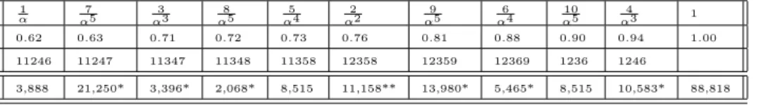
Example 1.22. Table 1 presents the (1,10)-parition and other useful information.
Lemma 1.23. For a fixed a≥1, b≥2,(a, b)−partition,hBi : 1≤i≤b+ 1i,and a realy∈[Bm, Bm+1),1≤m≤b,
TB(a,b)m =Ty(a,b). (1.12)
Proof. [1, Proposition 2.15].
Example 1.24. x=x(1,1,10) = 0.8.Inspecting Table 1, x∈[B6, B7) = [0.76,0.81).
It is then straightforward to verify, as shown in Table 1, that
T0.8(1,10)=h1,2,3,5,8i=T1(1,10). (1.13)
1
α 7
α5 3
α3 8
α5 5
α4 2
α2 9
α5 6
α4 10
α5 4
α3 1
0.62 0.63 0.71 0.72 0.73 0.76 0.81 0.88 0.90 0.94 1.00
11246 11247 11347 11348 11358 12358 12359 12369 1236 1246
3,888 21,250* 3,396* 2,068* 8,515 11,158** 13,980* 5,465* 8,515 10,583* 88,818
Table 1: Row 3 of this table contains the ten base 10, 1- Tojaaldi sequences of size at least 1. Row 4 presents the nu- merical frequencies of Tojaaldi sequences. Row 1 contains the (1,10)-partition of [α−1,1) by Bi,1 ≤ i ≤ b, defined in Defini- tion 1.17. Row 2 contains two digit numerical approximations of the Bi. In row 4, the number of asterisks indicate the differ- ence between (actual) observed and Benford (predicted) frequen- cies, 88818· log(Blog(1)−log(αi+1)−log(B−1)i).To illustrate our notation, there are 11158 occurrences of the Tojaaldi sequenceh1,2,3,5,8iamong the Tojaaldi sequences of sizes 1 to 88818. The Benford densities de- scribed in Definition 1.28 and Proposition 1.29, predict there should be88818· log(9)−log(α
5)
− log(2)−log(α2)
log(α) ≈11156occurrences, and
hence we have placed two asterisks on the 11158 entry to indicate a difference of two between the observed and predicted frequencies.
In the sequel we will assume integers a, bare fixed. This will allow us to ease notation and drop the functional dependency ona, b.So for example we will speak aboutk1instead ofk1(a, b).
In the sequel we will speak about an integer K≥k1(a, b).In several proofs we will speak about the effect ofK growing arbitrarily large.
Definition 1.25. The sequence{y(k)}k≥K, is recursively defined by
y(K) =x(K) = Fn(K)(a) bK , y(k) =y(k−1)
(αj+1
a
b , ify(k−1)αj+1ab <1,
αja
b , ify(k−1)αj+1ab >1, fork > K. (1.14) Definition 1.26. The sequence{ny(k)}k≥K,is defined byny(k) = 0,for k < K, and
ny(k) =ny = #{K≤i≤k:y(i)αj+1a
b >1}, k≥K. (1.15) Lemma 1.27.
y(k) = Fn(K)(a) bK
αja b
k−K
αnay(k−1), fork≥K. (1.16) Proof. A straightforward induction.
Definition 1.28. The sequence{nx(k)}k≥K, is defind by nx(k) = 0, fork < K, and
nx(k) = #{K≤i≤k:x(i)αj+1a
b >1}, k≥K. (1.17) Remark 1.29. The definitions and propositions we have just presented are almost identical to those in [1, Section 3]. The sole difference is that [1] restricts these definitions and propositions to the caseK=k1while here, we have allowedK > k1. It is this small subtlety which will allow us to prove that mostx(k)are arbitrarily close toy(k)for large enoughk > K.
Example 1.30. Leta= 1, b= 10.Thenk1(a, b) = 1.By (1.14) and (1.8),
{y(1), . . . , y(4)}={F6
10 = 0.8,0.8872,0.9839,0.6744} ≈ {x(1), . . . , x(4)}={ 8
10, 89 100, 987
1000, 6765 10000}. Note thatx(i)−y(i)≈0.003.
Definition 1.31. An integer k≥K will be calledexceptional relative to(a, b)if nx(k−1)6=ny(k−1).Otherwise,kwill be called non-exceptional.
Example 1.32. leta= 1, b= 10.Thenj(a, b) = 4andn(1, a, b) = 6.
By Definition 1.14,x(44) = F1021244 = 0.9034,to four decimal places. By Definition 1.21,y(44) = 0.9006.Buty(44)α105a = 0.9988<1,whilex(44)α105a = 1.0019>1, and consequentlyx(44)6=y(44),implying by Definition 1.26 that 45 is exceptional.
Note, that by Definition 1.21,y(45) = 0.9988.while by Definition 1.14,x(45) = 0.6192.
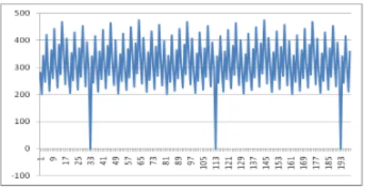
Hence, for the exceptional value of 45, x(45)and y(45)are not close. In fact, y(45)−x(45)>0.37.The "spikes" in Figures 1 and 2 correspond to the exceptional integers and show that they are rare.
Figure 1: Distribution ofbx(n)−y(n)1 + 0.5cfor2≤n≤200,for the 1-Fibonacci numbers and base 10. Thex(n) andy(n) are defined
in Definitions 1.14 and 1.21 respectively.
Figure 2: Distribution ofbx(n)−1y(n)+ 0.5cfor2≤n≤200,for the 2-Fibonacci numbers and base 10. Thex(n) andy(n) are defined
in Definitions 1.14 and 1.21 respectively.
Definition 1.33. Let[a, b)be an interval on the real line and let
X∼U nif orm([a, b))be a random variable uniformly distributed over this space.
If for some constant c >1, the random variable Y satisfies Y = cX, c >1, over the space[ca, cb),then we say thatYis Benford distributed over[ca, cb), and we notationally indicate this byY∼Benf ord([ca, cb).
Lemma 1.34. If Y∼Benf ord([ca, cb),then for ca ≤c1≤c2≤cb,
P rob(c1<Y< c2) =logc(cc2
1) b−a .
Remark 1.35. For a proof see [1, Proposition 4.3]. For general references on the Benford distribution see the bibliography in [1]. Notice that the restriction of the spaces and random variablesYandXto spaces of countable dense subsets of[a, b) does not change the proposition conclusion.
Example 1.36. Table 1, which presents 88,818 Tojaaldi sequences, allows illus- tration of the Benford sequence (and Conjecture 2).
Each of these 88,818 Tojaaldi sequences involve 4 or 5 Fibonacci numbers. Thus the 88,818 Tojaaldi sequences involve3888×5+21250×5+. . .+10583×4 = 424992 Fibonacci numbers. Since the Fibonacci numbers are Benford distributed, weexpect log10(109)×88818 = 19446.6Fibonacci numbers beginning with 9. Buth1,2,3,5,9i andh1,2,3,6,9iare the only Tojaaldi sequences having Fibonacci numbers begin- ning with 9; so we observe 13980 + 5465 = 19445 Fibonacci numbers beginning with 9.
We can repeat this numerical exercise for each digit (besides 9). We can then compute the χ−square statistic, χ2 = P9
i=1
(Oi−Pi)2
Pi = 0.0004 showing a very strong agreement between theory and observed frequency for the Fibonacci-number frequencies.
Similarly, as outlined in the caption to Table 1, we may computeobserved and expectedTojaaldi-sequence frequencies; the associatedχ−square statistic is 0.0013, suggesting that the Tojaaldi sequences are Benford distributed. This numerical
study motivates Conjecture 2 which will be formally stated in the next section and proven in the final section of this paper.
Definition 1.37. The uniform discrete measure used when making statements about frequency of Tojaaldi sequences on initial segments of integers, is given by the following discrete probablity measure.
PL(Tk(a,b)0 ) = #{k:Tk(a,b)=Tk(a,b)0 ,1≤k≤L}
#{Tk(a,b): 1≤k≤L} , L≥1, (1.18) with#indicating cardinality andk0, k, Lare integers.
2. Main theorems and conjectures
Conjecture 1. For allb≥2, a≥1,#T(a,b)=b.
Theorem 2.1. Forb >1, and arbitrarya≥1,
#T(a,b)≤b.
Proof. [1, Theorem 2.9]
Lemma 2.2. For given (a, b) let hBi : 1≤ i≤ b+ 1i be an (a, b)-partition, and letz0 be an arbitrary point in the real space[α−a1,1) with the continuous uniform measure. Then
P rob(Tz=Tz0) = µ([Bi, Bi+1)) µ([α−a1,1)) , wherei is picked so that[Bi, Bi+1) containsz0.
Proof. [1, Theorem 4.1]
Theorem 2.3. For any integerK≥k1, {y(i) :i≥K} is Benford distributed over the space[α−1,1).
Proof. [1, Theorem 4.5] (withK replacingk1 throughout the proof.) Conjecture 2. The{x(i)}i≥k1 are Benford distributed.
3. Proof of the two conjectures
In this section we prove the two main conjectures which we restate as theorems.
Prior to doing so we will need some preliminary propositions.
Lemma 3.1. {ny(k)}k≥K is non-decreasing and unbounded ask goes to infinity.
Proof. By Definition 1.22,ny(k)is non-decreasing. Suppose contrary to the propo- sition there is ak0 such that for allk≥k0, ny(k) =ny(k0).We proceed to derive a contradiction, proving thatny(k)is unbounded askgoes to infinity.
First, we show, using an inductive argument, thaty(k)∈(α−1a ,1), fork > K.
The base case, whenk=K is established by Definition 1.21 and equation (1.10).
The induction step is established by Definitions 1.21 and 1.8.
Returning to the proof of Proposition 3.1, note that according to Definition 1.21, there are two cases to consider, according to whether y(k0)αj+1ab < 1, or y(k0)αj+1ab > 1. We assume y(k0)αj+1ab < 1, the treatment of the other case be- ing almost identical. Then since we assumed ny(k) = ny(k0), k ≥ k0, we have y(k0)αj+1
a
b
n
<1, for all integern≥0, a contradiction, since by Definition 1.8, αj+1
a
b
n
goes to infinity as ngets arbitrary large. This contradiction shows that our original assumption thaty(k)is bounded is false. This completes the proof.
Lemma 3.2. For non-exceptional k > K
|x(k)−y(k)| ∈
α−2n(K)−1a , α−2n(K)a
. (3.1)
Proof. [1, Proposition 3.6] withK replacing k1 in both the proposition statement and throughout the proof.
Remark 3.3. As noted in the previous section, because we replaced k1 by K, the lower bound estimate of the difference in (3.1) is going to 0. Consequently {x(i)}i≥K is asymptotically approaching {y(i)}i≥K.Formally, we have the follow- ing Corollary.
Corollary 3.4. As kvaries over non-exceptional k,
klim→∞|x(k)−y(k)|= 0.
Proof. Immediate, by combining Propositions 3.1 and 3.2.
Lemma 3.5. Using Definition 1.17, lethBi: 1≤i≤b+ 1i=h1, i
αe(i)a
: 1≤i≤bi be an(a, b)-partition. Then the#{TBi,1≤i≤b}=b,that is, theTBi are distinct.
Proof. Following [1, Proposition 2.15], define a b×j(a, b) + 1 matrix, A(k, l) = Bkαla,1≤k≤b,1≤l≤j(a, b) + 1,so that by Definition 1.13
TBk =hbA(k,1)c, . . . ,bA(k, m)ci, and by Definitions 1.16, 1.17 and 1.8, m equals j(a, b)orj(a, b) + 1. Recall the following facts about the matrixA:
(I) A(k, e(i(k))) = i(k); (II) no other cell entries (besides (k, e(i(k)))) can have exact integer values; (III)A is strictly increasing as one goes from top to bottom and left to right, that is,A(k, l)< A(k0, l0)if either (i)l < l0 or (ii)l=l0, k < k0.
Using these three facts we see that bA(k0, e(i(k))c< A(k, e(i(k)), for k0 < k, 1≤k≤b, i(k)6=b.Hence,TBk0 6=TBk,for k0 < k.An almost identical argument applies wheni(k) =b.Hence theTBi are distinct as was to be shown.
Example 3.6. We can illustrate the proof using Table 1. By Table 1, B4 = α85, implying that the 5th member of the sequenceTB4 equals 8 and the 5th member of the previous sequences,TBk,1≤k <4,are strictly less than 8 as confirmed by Table 1.
Note also the special case B9 = α105, implying that the 5th member of the sequenceTB9 is empty while the 5th member of the previous sequences, TBk,1≤ k≤8,are non-empty, as confirmed by Table 1.
The next three propositions show that exceptional k (as defined in Definition 1.26) are rare. First we prove the following proposition, which provides an alternate recursive definition tox(k),defined in Definition 1.14.
Lemma 3.7. The sequence {x(k)}k≥K,is recursively defined by
x(K) = Fn(K)(a) bK ,
x(k) =
x(k−1)α
j+1 a
b +Fj+1(a)β
n(k−1) a
bk , ifx(k−1)α
j+1 a
b <1, x(k−1)α
j a b +Fj(a)β
n(k−1) a
bk , ifx(k−1)α
j+1 a
b >1, fork > K.
(3.2)
Proof. If k = K the proposition is true by Definition 1.14. If k > K, then by Definitions 1.3, 1.7 and Proposition 1.10
n(k)−n(k−1) = #Tk(a,b)−1 ∈ {j, j+ 1}.
Consequently, there are two cases to consider. We treat the casen(k) =n(k− 1) +j, the treatment of the other case,n(k) =n(k−1) +j+ 1,being similar.
But then, by Proposition 1.12,
Fn(k)(a) =αjaFn(k−1)(a) +Fj(a)βn(ka −1).
Equation (3.2), follows by dividing both sides of this last equation bybk and ap- plying Defintion 1.14.
Prior to stating the next two propositions, it may be useful to numerically illustrate the proof method. The following example continues Example 1.27.
Example 3.8. Leta= 1, b= 10.Then by Definition 1.8,j(a, b) = 4.By Definitions 1.22 and 1.24,
ny(43) =nx(43),
implying by Definition 1.26, that 44 is not exceptional. By Definition 1.21,y(44) = 0.9006;by Definition 1.14,x(44) = 0.9034.Application of Defintions 1.22 and 1.24 require use of α105a = 0.9017.Observe that
y(44) = 0.9006<0.9017<0.9034 =x(44).
Consequently,
y(44)α5a
10 <1;x(44)α5a 10 >1.
Therefore, by Definitions 1.22 and 1.24
ny(44) =ny(43) + 1;nx(44) =nx(43).
Hence, by Definition 1.26, k= 45 is an exceptional value. Notice that y(44)and x(44) are close in value as predicted by Proposition 3.2. The values ofx(45)and y(45)may now be computed using Definition 1.22 and Proposition 3.6,
y(45) = 0.9988;x(45) = 0.6192.
Here,y(45)andx(45)are not close. More precisely,y(45)is close to 1 whilex(45) is close toα−1a .
But by applying Definitions 1.22 and 1.24 we see that ny(45) =ny(44);nx(45) =nx(44) + 1, implying that
ny(45) =nx(45),
in other words, 46 is not exceptional. We in fact confirm thaty(46)andx(46)are indeed close as required.
y(46) = 0.6846<0.6867 =x(46).
We may summarize this numerical example as follows: (I) Most k are non- exceptional. (II) For an exceptionalk to occur, one ofx(k−1), y(k−1) must be greater than αj+1ab while the other is less. (III) This occurs rarely because most k are non-exceptional and hence, by Proposition 3.2, x(k) and y(k) are usually numerically close. (IV) If k is exceptional then x(k) will be close to α−1a while y(k)will be close to 1. (V) Consequentlyk+ 1will not be exceptional and in fact x(k+ 1)andy(k+ 1)will again be close to each other.
The next proposition formalizes this example.
Lemma 3.9. If k is exceptional thenk−1andk+ 1 are non-exceptional.
Proof. Assume thatkis exceptional andk−1is not exceptional. This assumption is allowable, since by Definitions 1.21, 1.22 and 1.24,KandK+1are not exceptional and therefore the "first" exceptionalkmust be preceded by a non-exceptional value.
We proceed to show thatk+ 1is not exceptional. Therefore, the "2nd" exceptional k is preceded by a non-exceptional k. Proceeding in this manner we will always be justified if we assume the predecessor of an exceptional k is not exceptional.
Consequently, we have left to prove thatk+ 1 is not exceptional.
By Definitions 1.26, 1.22 and 1.24, forkto be exceptional we must have one of x(k−1)αj+1ab and y(k−1)αj+1ab greater than one while the other is less than one.
We treat one of these cases, the treatment of the other case being similar.
Accordingly, we assume
ny(k−2) =nx(k−2)−→ k−1is not exceptional, (3.3)
and we further assume y(k−1)< αj+1a
b −1
< x(k−1)−→y(k−1)αj+1a
b <1, x(k−1)αj+1a
b >1. (3.4) Combining Proposition 3.2 with (3.4) we obtain
y(k−1)> αj+1a b
−1
− 1 α2n(K)a
, x(k−1)< αaj+1 b
−1
+ 1
α2n(K)a
. (3.5)
Hence, by Definition 1.21 and Proposition 3.6, y(k) =y(k−1)αj+1a
b , x(k) =x(k−1)αja
b +Fj(a)βan(k−1)
bk . (3.6)
Using equation (3.4), Definitions 1.26, 1.22 and 1.24, we confirm that
ny(k−1) =ny(k−2), nx(k−1) =nx(k−2) + 1−→kis exceptional. (3.7) Again, by Definition 1.26, to decide whether k+ 1 is exceptional we need to computeny(k)andnx(k).We first compute ny(k).
Appplying equations (3.6) and (3.5) to Definition 1.22, we have y(k)αj+1a
b =y(k−1) αj+1a b
2
> αaj+1
b − α2j+2a b2α2n(K)a
. (3.8)
j and b are O(1) (relative to the choice of K) while we may chose K arbitrarily large. It follows that asKgoes to infinity,
y(k)αj+1a
b >αj+1a
b − α2j+2a
b2α2n(K) ≈αj+1a
b >1. (3.9)
Consequently by (3.9), Definition 1.22, and (3.7)
ny(k) =ny(k−1) + 1 =ny(k−2) + 1. (3.10) . We now carry out a similar analysis on x(k).By Proposition 3.6 we have
x(k)αj+1a
b = x(k−1)αaj
b +Fj(a)βan(k−1)
bk
αj+1a
b (3.11)
Applying the upper bound for x(k−1) presented in (3.5) we obtain after some straightforward manipulations
x(k)αj+1a b <αja
b +α2j+1−2n(K)a 1
b2 +Fj(a)α(j+1)a βan(k−1)
bk+1 ≈ αja
b <1. (3.12) Hence, by Definition 1.24 and equation (3.7),
nx(k) =nx(k−1) =nx(k−2) + 1. (3.13) Equations (3.10) and (3.13) together imply that nx(k) = ny(k), and hence, by Definition 1.26,k+ 1is not exceptinoal as was to be shown.
This completes the proof.
Lemma 3.10. P rob({k:k is exceptional}) = 0.
Proof. By Proposition 3.8, exceptionalk occur as singletons (that is, two consec- utive integers cannot be exceptional). Furthermore, by Proposition 3.2, if k is exceptionalk−1 is non-exceptional and
x(k−1), y(k−1)∈ αj+1a b
−1
− α2n(K)a −1
, αj+1a b
−1
+ α2n(K)a −1 . By Theorem 2.3 the{y(i)}i≥K are Benford distributed and hence the probability ofy(k−1)being in an open interval whose width is going to 0, may be made as small as we please.
But by Proposition 3.8 every exceptionalk is uniquely associated with a non- exceptionalk.
This completes the proof.
We can now prove the two conjectures.
Theorem 3.11. The {x(n)}n≥1 are Benford distributed.
Proof. Consider an arbitrary set (of reals), B ⊂ (α−a1,1). To prove the theorem, we must show that P rob(B∩ {x(n)}n≥1) equals the desired Benford-distribution probability.
By Definition 1.28 and Proposition 1.29 we know thatP rob(B∩ {y(n)}n≥1) =
log(My)−log(my)
log(1)−log(α−a1) , with My = sup (B∩ {y(n)}n≥1) and my = inf (B∩ {y(n)}n≥1). Define Mx = sup (B∩ {x(n)}n≥1) and mx = inf (B∩ {x(n)}n≥1). By Corollary 3.3,|My−Mx|and|my−mx|can be made arbitrarily small. The result immediately follows.
Theorem 3.12. For allb≥2, a≥1, #T(a,b)=b.
Proof. By Theorem 2.1, #T(a,b) ≤ b. It therefore suffices to prove #T(a,b) ≥ b.
The proof is constructive.
Using Definition 1.17, let hBi : 1 ≤i ≤ b+ 1i = h1, i
αe(i)a : 1≤ i ≤bi be an (a, b)-partition. For1≤i≤b,pick a non-exceptionalx(ni)∈(Bi, Bi+1),for some integerni. x(ni) exists since by Theorem 3.7, {x(n)}n≥1} is Benford distributed and hence dense in(α−a1,1).
But then by Proposition 1.19, Tx(ni) = TBi; by Proposition 3.4, the TBi are distinct; and by Proposition 1.15,Tx(ni)=Tni.Hence, we have produced at least bdistinct Tojaaldi sequences as was to be shown.
References
[1] Tom Barrale, Russell Hendel, and Michael Sluys Sequences of the Initial Digits of Fibonacci Numbers, Proceedings of the 14th International Conference on Fibonacci Number, (2011), 25-43.