State-space Analysis of the Interval Merging Bi- nary Tree
Istv´an Finta
Nokia, Bell Labs
H-1083, Budapest, B´okay street 36-42 istvan.finta@nokia-bell-labs.com
S´andor Sz´en´asi
Obuda University´
H-1034, Budapest, B´ecsi street 96/b szenasi.sandor@nik.uni-obuda.hu
Abstract: In the course of transmission through networks a particular packet, like a Storm tuple or a performance/fault management (PM/FM) report in XML format of an Operation Support System (OSS) application, data loss/out of order arrival/duplication phenomena may cause the packet not to arrive at the destination, arrive exactly once or to arrive in several copies. These anomalies have to be handled both on the lower and higher level network or application layers to an extent depending on the later usage. The efficiency of handling de- pends on the applied data structures.
To detect packet loss and duplication, a special, tree-like data structure was proposed earlier, the Interval Merging Binary Tree (IMBT). We analyzed IMBT from several perspectives and we compared its performance with other well-known tree variants, under various circum- stances. However, in contrast to a completely balanced binary search tree, it is impossible to associate to the newly developed data structure a one dimensional function, dependent on the number of input keys, to determine for instance the average cost of an operation. Never- theless, for further development, it is essential in case of any data structure, to determine the actual boundaries of its applicability.
In this contribution we explore the state space of IMBT in order to be able to classify the data structure regarding the input pattern during the later performance analysis. We used in the modeling Fibonacci sequences, bipartite multi-graphs and combination tables.
Keywords: data structure; balanced binary tree; bipartite graph; fibonacci sequence; state space; combination table;
Introduction
Performance management is an OSS application in which performance measure- ment records, generated periodically by network elements, are processed in order to assess the performance of the network. Each record consists of performance-related counters (key + value) each describing a specific aspect of the performance within a period. The periodicity of records makes it possible to associate incremental keys to the individual counters from the records, where the value is the content of the counter itself. The percentage of lost records is typically very low, therefore rela- tively few counters are lost in the transmission. Counters are converted into Key Performance Indicators (KPI-s) via Extract Transform Load (ETL) functionality for which we used Storm [2], a stream processing engine. Because of the at-least-once processing pattern of Storm, duplicated and out-of-order keys might occur. Packet loss and duplication of raw measurement data will lead to errors when aggregat- ing counters into KPI-s, conveying a wrong perspective about the performance of the network, therefore loss and duplication cannot be tolerated in this particular use case.
In order to decide in real time whether a counter is identified by a key has al- ready arrived or not and to insert it if not, we need a space-efficient data structure which is fast searchable and allows fast insertion of keys. After careful consid- erations, we ruled out a number of alternatives. The examined alternatives were external databases, Bloom filter [3], Balanced BSTs[4] [5], hash tables [4]. Ex- ternal databases turned out to be too slow. We ruled out Bloom filters because it allows false positives: for a key reported to be present we know only with certain probability its true presence in the data structure. This uncertainty is not allowed in our case. Balanced BSTs were ruled out due to their linearly increasing space need, which is proportional with the number of handled keys by them so far. The proportionally increasing space need was a drawback regarding hash tables as well.
Additionally the need for periodical ’re-hashing’ in an upper-unbound environment would also significantly decrease the computation performance. Finally we arrived to proposing an efficient data structure and associated algorithms that we called In- terval Merging Binary Tree (IMBT)[1].
In the unpublished [6] we have examined several tree layout instances and extreme scenarios for the arrival pattern of keys. Additionally we have deducted the formu- las regarding the cost of SEARCH operation, as the basis of other operations, like INSERT or REMOVE. We have examined both theoretically and experimentally the performance of IMBT for an exponential distribution of the key arrival pattern [7]. Until now if onlyN, the number of IMBT handled keys, was given, we could not estimate nor even model accurately the state space of IMBT. State space mod- elling can facilitate the mapping of the statistical distribution-based input patterns into the IMBT state classes, if these exists at all. In the more general interpreta- tion of state space we mean anN-dependent numerical value that characterizes the BST, and with normalization by Na statement can be made regarding the cost of operations. In case of traditional BSTs if the tree arrangement is given, then we can easily determine thatN-dependent value which is the base of metrics like aver- age time complexity of SEARCH operation etc. However, in contrast to traditional
BSTs, the IMBT state space is a multivalued function ofN.
Therefore the analysis is divided into the following sections, through which we will unveil the aspects affecting theNmultivalued dependency.
In sectionBasics of the Interval Merging Binary Treewe briefly introduce the IMBT data structure. From the description it will be clear that the analysis of the tree can be split into two independent aspects. In sectionInterval State Spacewe will show the relation between the possible number of arrangements of intervals across the tree and the Integer Partitions [8]. This is the first aspect.
The second aspect will be introduced in section Traversal Strategy Based Weight Classes. In this section we will describe the relationship between IMBT and a priv- ileged tree arrangement, the completely balanced binary search tree. Here we will highlight the relationship between the Fibonacci sequences [9] and the number of comparisons required to reach a set of intervals within IMBT. In case of not limiting the examination to the completely balanced trees, according to Caylay’s theorem [10]nn−2different tree arrangements should be considered, wherenis the number of nodes in a tree, which is impractical and turns out not to be needed.
In sectionBipartite Graphs and Combination Tableswe combine the two approaches into one model. During the combination we would like to determine the possible number of different values, which represents in fact the state space. In case when we just simply multiply the number of integer partitions ofN with the different num- ber of ”step classes”, then we get many duplicate values. That is, the state space would be highly overestimated. To mitigate this, we will introduceG(I,W)bipar- tite graphs as a representation. In the course of matrix representation of the graphs we will apply a simplification and we can show that the result is nothing else than a combination table. The degrees of freedom of a combination table is a huge number.
Regarding the enumeration of non-conform combination tables, orG(I,W) graphs in our case, there are available results like [11], or [12], but as will be shown in our case both sides of the table increase deterministically, according to integer partitions and Fibonacci sequences. In our work we will also apply an additional equal trans- formation, like in the previous two references, to be able to formulate the criterion to get such sum of two members multiplications where the duplicates are minimized or zero. Therefore our result can be considered as an upper bound of the state space of IMBT in case whenNis given.
Basics of the Interval Merging Binary Tree
IMBT is a data structure of disjoint sets, organized into a tree. The speciality of the sets is that each must contain all the keys between the greatest and the lowest value of a particular set. Sometimes these type of sets are called integer interval, hence we named the data structure interval merging binary tree, where merging refers to the operation of immediate merging 2 disjoint sets that become joint as a result of an incoming key.
As stated in theIntroduction, we assume an input stream of keys where the key is a sequence number. Keys are arriving mostly ordered respective to the sequence num- ber. The task is to filter out those entries that arrived already once, meaning that the
sequence number has had already this value in an earlier key instance. Additional boundary conditions regarding the arrival pattern apply:
1. upper unbounded range: there is no upper bound of the sequence numbers apart from the limit of the binary representation of this field,
2. lower unbounded range: at any point in time a new key can arrive to the system with a sequence number lower than any sequence number encountered so far,
3. there are long, contiguous intervals of keys with relatively few ’gaps’ (missing keys) in between,
4. after a while almost all keys arrive,
5. key duplication (i.e. same key arrived at least twice) on the arrival side is possible due to some reason.
Let’s suppose that keys arrive to IMBT in the following order:
...k0,k−1,k2,k3,k7,k5,k4,k6,k−2, ...
According to a naive approach all elements should be stored in a hash or in a binary search tree which is easily searchable, but still the binary search tree or the hash remains an upside-downside open system with infinite storage requirements when keys can arrive with infinite delay.
The first tweak to the naive approach is to represent the arrived keys as pairs. So, elements will be stored like the following:
(k0,k0),(k−1,k−1),(k2,k2),(k3,k3),(k7,k7),(k5,k5),(k4,k4),(k6,k6),(k−2,k−2).
At first sight it looks like that we did not win anything, but only doubled the memory footprint. The second tweak is not to automatically put newly arrived elements at the end, but rather to organize the elements in an ordered fashion, filtering at the same time duplicates found during the ordering process. This can be conceptually a sequence of 3 operations: insert at the end, order by key and a filter to skips the entry if it is already found:
(k−2,k−2),(k−1,k−1),(k0,k0),(k2,k2),(k3,k3),(k4,k4),(k5,k5),(k6,k6),(k7,k7).
The third tweak is to add an operation that we call interval merging: every pair of neighbour values is checked and if the values are consecutive, the two pairs are converted into one, where the first value of the resulting pair is the first value of the first pair and the second value of the resulting pair is the second value of the second pair. The skeleton code is available in [1].
In the following we describe the operation of the algorithm for our small data set:
• k0arrives, our data structure will store the following element:
(k0,k0)
• k−1arrives, our data structure will store the following element:
(k−1,k0)
• k2arrives, our data structure will store the following elements:
(k−1,k0),(k2,k2)
• k3arrives, our data structure will store the following elements:
(k−1,k0),(k2,k3)
• k7arrives, our data structure will store the following elements:
(k−1,k0),(k2,k3),(k7,k7)
• k5arrives, our data structure will store the following elements:
(k−1,k0),(k2,k3),(k5,k5),(k7,k7)
• k4arrives, our data structure will store the following elements:
(k−1,k0),(k2,k4),(k5,k5),(k7,k7)
Then
(k−1,k0),(k2,k5),(k7,k7)
• k6arrives, our data structure will store the following elements:
(k−1,k0),(k2,k6),(k7,k7)
Then
(k−1,k0),(k2,k7)
• k−2arrives, our data structure will store the following element:
(k−2,k0),(k2,k7)
So, at the end storing only two intervals are required to represent 9 arrived keys.
In case of we would organize these intervals into a binary tree then, as mentioned in the Introduction, the IMBT search operation state space would be influenced from two different aspects:
– the length of the intervals,
– the steps/comparison required to find that interval, that is the position of the interval within the tree.
In the following section we will examine the role of the intervals in the state space analysis of IMBT.
Interval State Space of IMBT
Fig.1, Fig.2 and Fig.3 indicate various types of evolutions of the tree as a function of the incoming keys, where in all cases we have 4 input packets.
Figure 1
IMBT interval evolving when no direct neighbour exists.
On the figureNrepresents theTtime as well. By looking to the figure from the right side, the remaining axes display a histogram of the intervals in different moments.
Figure 2
IMBT interval evolving when the keys are subsequent
As it is visible in case of four keys (N=4), based on the possible number of neigh- bours, the following scenarios can be distinguished:
– None of the keys are neighbour of each other, like Fig.1, – Two of them are neighbours and the other two are not, – Two of them are neighbours and the remaining ones as well,
Figure 3
IMBT interval evolving when there are both neighbour and stand alone keys
– Three of them are neighbour and one is not, like Fig.3, – All the keys are neighbour of each other, like Fig.2.
Therefore we can say that according to Hardy and Ramanujan [8]:
Theorem1. the number of possible interval states in case of IMBT, atT =Ntime, is equal with the number of waysNcan be written as a sum of positive integers:
N→∞lim p(N)≈ 1 4N√
3eπ
√
2N/3 (1)
We can identify the addends of the sum as the individual interval lengths of the nodes in the IMBT. In this case for the average interval lengthsa, considering the list items above, we get the following values, respectively: 4/1=4, 4/2=2, 4/2=2, 4/3, 4/4=1. As it is visible there are two equivalent values: 2. Therefore it is generally true that the number of integer partitions is a rough upper estimation regarding the possible number different averages for a given input sizeN.
Additionallyp(N)does not say anything about the weight of the intervals based on their position in the tree. Since the same decomposition may led to very differently weighted arrangements it matters if for instance the intervals of 8 is written in e.g..:
1+1+4+1+1 or 4+1+1+1+1 or 1+1+1+1+4 form. Supposing that the intervals are organized into a balanced binary search tree, the cost of the search operation in the first case is the most favourable, and in the last case is the least favourable. To account for these differences, in Traversal Strategy Based Weight Classeswe will factor the transversal strategies in our analysis.
Traversal Strategy Based Weight Classes
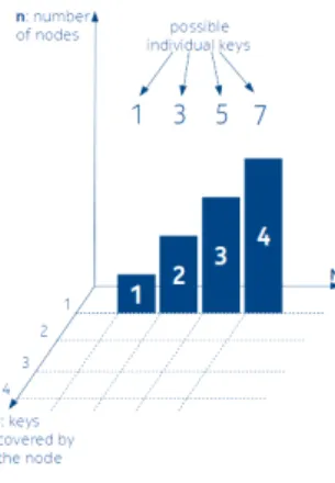
In Fig.4 the arrows with number represent the jthcomparison during the SEARCH operations. Here we would like to mention that, for the sake of simplicity, during the comparisons the less or equal will be considered as one atomic step. The dark
Figure 4
IMBT weight classes caused by the traversal strategy
background of the number expresses that the result of the comparison can be posi- tive (that is, the node covers more than one key). In this figure, instead of boundaries of the intervals, the same information is displayed in the nodes as on the arrows.
As we can see if the key to be searched for is equal with the left hand value of the root node then exactly one comparison will be performed. If the key to be searched for is in between the left and right hand values of the root node or equal with the right hand value then two comparisons will be performed.
If the key is greater than the right hand value of the root node and falls into the interval of the right hand child’s left and right hand values then three or four com- parisons are required, depending on the exact value.
If the key is less than the left hand value of the root node and falls into the interval of the right hand child’s left and right hand values then two or three comparisons are required, depending on the exact value.
By continuing the examination of the distribution of the different classes of inter- vals, based on the required number comparisons, we can recognize the following rules, when the intervals are organized into a completely balanced tree.
Considering the root (first) level there is one such interval where(1,2)compari- son can occur. In the second level there is one interval where(2,3)and one inter- val where(3,4)comparison(s) can occur. Finally, in the third level the cumulated number of intervals where(1,2)and(2,3)comparison(s) can occur is unchanged.
However, the number of(3,4)comparison intervals is increasing from one to two.
Additionally two(4,5)and one(5,6)comparison intervals appear.
By the cumulative number of types, as more and more layers are taken into account, we will get the pattern described in Table-1. Examining carefully the lists we can realize that
Theorem2. the central element of each row composed from cumulative number of weight types is the Fibonacci sequence itself. The numbers in the lists (lines in this case), preceding the central elements, are also the evolving Fibonacci sequences themselves. The rest of the numbers must satisfy the requirement that the sum of the numbers is equal with 2n−1 in everynthline.
However, another rule also can be recognized there:
Theorem3. the numbers in a line from Table-2 are equal to the sum of the two preceding numbers of the previous line.
Table 1
Distribution of weight classes in case of the IMBT is completely balanced.
The Fig.4 snapshot is marked with bold.
Distance from the root
Total number [number of comparisons
of nodes in IMBT regarding the left hand value]
1 2 3 4 5 6 7 8 9 10 11
1 1
3 1 1 1
7 1 1 2 2 1
1515
15 111 111 222 333 444 333 111
31 1 1 2 3 5 7 7 4 1
63 1 1 2 3 5 8 12 14 11 5 1
Table 2
Fibonacci sequences in the cumulated weight classes
111
1 111 1
1 1 222 2 1
1 1 2 333 4 3 1
1 1 2 3 555 7 7 4 1
1 1 2 3 5 888 12 14 11 5 1
Until now we have shown that there are two distinct aspects influencing the state space of IMBT. One is if how many ways the number of keys can be decomposed into integer partitions.
The second aspect is represented by the weight classes. It is based on the number of nodes and depends on the associated traversal strategy.
Now, to be able to determine the combined number of input pattern classes some- how we have to put these components together. InBipartite Graphs and Combina- tion Tables on the modeling of IMBT State Spacewe will present this combination procedure and the resulting mathematical models.
Bipartite Graphs and Combination Tables on the mod- eling of IMBT State Space
To be able to start the combined analysis we will perform the following mappings.
Let’s denote the length of the interval belonging to anninode from the IMBT by li∈L, whereLis a multi-set. Then we map the set of same length of intervals onto i1,i2, ...,ik∈Ielements. This means that by having theL={l1,l2, ...,ln}lengths, where the values oflh=li=...=ljis equal, then this fact results in one new el- ement, ip, in theIset. That is the followinglh→ip,li→ip,lj→ipsurjection is performed in case oflh=li=lj. Thereforek≤n.
Let’s denote the number of comparisons required to achieve the left hand value of an arbitraryni node bysi∈S, whereS is a multi-set. Then let’s map the traver- sal strategy based identical comparison weight types ontow1,w2, ...,wj ∈W ele- ments. This means that by having theS={s1,s2, ...,sn}lengths, where the values ofsh=si=...=sj are equal, then this fact results in one new element,wp, in the W set. That is, the followingsh→wp,si→wp,sj→wpsurjection is performed in case ofsh=si=sj. Thereforek≤n.
Since the newly definedIandW are two disjoint sets we can consider them as the vertices of aG(I,W)bipartite (multi-)graph. We will assign degrees to each vertex in the following manner:
The degree of eachiivertex is equivalent with the number of those particular interval lengths. According to this in case oflh=li=ljthe degree of the associatediivertex isd(ii) =3.
The degree of eachwivertex is equivalent with the number of those particular weight types in the search tree.
Therefore we can write that
Theorem4. ∑i=1j d(wi) =∑ki=1d(ii) =n=|E|, whereE={e1, ...,en}is the set of theeiedges ofG(I,W).
The fact that the above two sets,I andW, are the independently different classifi- cations of the same nodes of the IMBT implies that the sum of the degrees of the vertices in both sets is equal ton.
Let’s consider an IMBT arrangement/configuration wheren=4, and bothIandW sets contain one-one vertex with degree two, and two additional vertices with degree one-one. So,d(i1) =d(w1) =2 andd(i2) =d(i3) =d(w2) =d(w3) =1. At this moment regardingNwe can only say thatN≥n.
It is obvious that to get the aboveIset two of the lengths must be equal, eg.l1=l2, and the other must differ from bothl1=l26=l3,l1=l26=l4andl36=l4.
Definition: ThoseLinterval length multi-sets are calledinterval lengths ratio base classes, denoted byLb, in which
at least one li exists which is co-prime to all the other lj, such thati6= j supposing thatli6=lj, or
ifli=ljfor alli6=j, thanli=lj=...=lk=prime number.
That is,Lis anLbif
∃li∈L|(∀i6= j∧li6=lj⇒gcd(li,lj) =1)∨ (∀i6=j ⇒li=lj=prime number).
(2) IfL={l1,l2,l3,l4} is an interval lengths ratio base class, that isL=Lb, thenLb determines all theN1,N2, ..., which differ from each other by only an integer factor for a given(Lb,n=|Lb|)pair. This representation/decomposition is unique, except
for the order of the factors:
Nx= (d(i1)×l1×x) + (d(i2)×l3×x) + (d(i3)×l4×x)
=x×(d(i1)×l1 + d(i2)×l3 +d(i3)×l4). (3) wherex∈ {1,2,3, ...}. Ifn is given that is the maximum information we can get regardingN.
In Fig.5 all the different possible configurations are shown for the aboveG(I,W), where|I|=|W|=3 and|E|=n=4. That is, there are three-three vertices on both sides of theGgraph.
Figure 5
G(I,W), where|I|=|W|=3 andn=4
At this stage we can claim thatN≥4. If we are aware of thel1,l2,l3,l4∈Lvalues, e.g.:l1=l2=1,l3=2 andl4=3 and thereforeL1=Lbthen we can say thatN1=7.
However,N2=14,N3=21, ...andL2,L36=Lb.
As it is visible from the Fig.5 there are seven different possible configuration. Re- garding the number of possible configurations, in case of a given(L,n)pair, till now we have a mathematical model asG(I,W)is a bipartite graph. We can formulate the following
Theorem5. The simplified adjacency matrix representation of aG(I,W), which is derived from an IMBT according to the above process, corresponds to a contingency table.
Let’s assume anG(I,W)bipartite graph derived from an IMBT. Let’s prepare the adjacency matrix of G(I,W), where parallel edges are allowed, in the following manner. SinceG(I,W)is a bipartite graph there are no edges between the vertices belonging to the same vertex set. Then we will apply the following simplification:
instead of enumerating all the points from both sets on the right side and the top of the adjacency matrix merely the points fromIwill be displayed with the associated d(ii)values on the right side. On the top of the matrix only the points fromW will be displayed with the associatedd(wj)and values.
The edges appear as numerical entries in the cells of the matrix. The value of a
particular cell represents the number of edges between theiiandwjpoints. However thed(ii)andd(wj)values are constraints regarding the sum of a givenirow and j column.
From Theorem 4we know that the sum of cells in a row is equivalent with the degree of that particular vertex. The same is true for all columns. Therefore the sum of sums of every row is equivalent with the sum of sums of every column.
This feature of the simplified adjacency matrix is corresponding to a contingency or combination table, which may contain discrete samples of the same multitude from two different points of view.
In Fig.6 the simplified adjacency matrix representation of theG(I,W)graphs from the Fig.5 is shown. Since the edges do not appear directly, the simplified adjacency
Figure 6
Simplified adjacency matrix of G(I,W)
matrix remains unchanged in case when two different,ekandel edges that are not sharing on any vertices on any of their ends, are mutually replaced with each other.
This holds also for the case when neighbours edges, sharing on a multi-degree ver- tex, replace their non-sharing ends with each other.
Therefore from this simplified adjacency matrix like it is still hard to establish the formal condition of states being different, that is the total weight of the IMBT. The number of states for a given (I,W) is the different number of total weights of the IMBT.
Nevertheless, we can apply the following transformation without violating the va- lidity of the transformed model. During the transformation we are composing so called domains in the matrix in a way that every row(or column) with valued(ii)(or d(wj)) will be substituted withd(ii)(ord(wj)) rows(or columns), where the con- straint value of each row is ’1’. Therefore the 1×1 cells, which are in the cross of thed(ii)row and thed(wj)column, will be replaced by such a domain that consists ofd(ii)×d(wj)cells.
In Fig.7 the domain composition of the aboveG(I,W)is visible, where the domains are marked/surrounded by dotted lines.
Figure 7
G(I,W) simplified adjacency matrix transformation to domain representation
In Fig.8 the domain transformed matrix representation of the Fig.5 examples are shown. The numbers with blue background mark the relatedG(I,W)from the ex- amples. Let’s denote the set of all theG(I,W)graphs belonging to the same partition
Figure 8
G(I,W) examples with domain representation.
The numbers with blue background marks the related G(I,W) from the above examples.
ofNbyPN,Li. From theInterval State Space Sectionwe know thati∈ {1...p(N)}. A particularGk(I,W)∈PN,Li expresses thenmembers sum of two members products, where the members of the products are from theLiandW sets respectively. There- fore theGk(I,W)∈PN,Lidetermined sum of products can be mapped onto the IMBT state space. Now we will define the subset ofPN,Li, denoted byPN,Ls
i, according to the following.
PN,Ls
i is the subset of thePN,Li set that contains the maximum number ofGi(I,W) graphs fromPN,Li, so that in theG(I,W)associated transformed matrices the sum of cells are different for all the(Gi,Gj)i6=jpairs in at least 4 domains.
Theorem6. |PN,Ls
i|is an upper bound regarding the possible number of IMBT states belonging to anN→Lipartition.
Let’s consider in the following lengthsl1,l2, ...lnand stepss1,s2, ...sn. Let’s addi- tionally assume that there are ielements from both the l’s and s’s where the as- sociated lengths and steps are equivalent with each other. Additionally there are two additional jandkelements from bothLandSwhere the associated values are the same andi+j+k≤n. Let the associated value of theielements be vi=2, vj=3 and vk=4. Then there will be such a G1(I,W)and G2(I,W) bipartite graphs that are identical in every other pairings regarding the member of the prod- ucts except theG1→r1=...+li,i×si,i+lj,1×sj,1+...+lj,j×sk,1+lk,1×sj,jand G2→r2=...+lj,1×si,i+li,i×sj,1+...+lk,1×sj,j+lj,j×sk,1. In this case(G1,G1) pair satisfies the above condition regarding the sum of domains, however the associ- atedr1andr1results are identical, therefore this represents the same state of IMBT.
From the above we can formulate the following
Theorem7. The upper bound of the IMBT state-space in case of knowing onlyN, and the samennumber of lengths are always sorted into the same tree structure no matter whatever it is:
IMBTStates(N) =|PN,Ls
1∪PN,Ls
2∪...∪PN,Ls
p(N)| ≤
p(N) i=1
∑
|PN,Ls
i|. (4)
In case of a completely balanced IMBT the degrees belonging to a particularwiare equivalent with the corresponding number from the corresponding line of Table-2.
For instance in case ofn=7 we can identify the third line of Table-2. Therefore we know that the number of different weights is 5. And the seven nodes are sorted into five classes according to the followingsd(w1) =1,d(w2) =1,d(w3) =2,d(w4) = 2,d(w5) =1.
Conclusions
In this contribution we have introduced a special tree structure, the IMBT. Then we have pointed out the aspects contributing to the state space of this data structure and we provided an upper bound for the cardinality of this state space.
Now we have a mathematical model through we can perform measurements and an assessment of a concreteG(I,W)representation to which a series of keys tends. This might be a possible classifier regarding the statistical distribution of the key arrival process. In the following we plan to determine some correlation/combination tables for different distributions.
References
[1] Finta, I., Farkas, L., Sergy´an, Sz., Sz´en´asi, S.: Interval Merging Binary Tree, ICA3PP 2017, Helsinki, Finland, August 21-23, 2017
DOI:10.1007/978-3-319-65482-9
[2] STORM - A distributed real-time computation system, http://storm.
apache.org/documentation/Home.html, last visited 2019-01-02
[3] Bloom, B. H.: Space/time trade-offs in hash coding with allowable errors, Communications of the ACM, Volume 13 Issue 7, pp 422-426, New York, NY, USA, July 1970.
[4] Cormen, T. H., Leiserson, C. E., Rivest, R. L., Stein, C.: Introduction to Algo- rithms (3rd ed.). MIT Press and McGraw-Hill, 2009.
ISBN:0-262-03384-4
[5] Bayer, R.: Symmetric binary B-Trees: Data structure and maintenance algo- rithms, Acta Informatica, Volume 1, Issue 4, pp. 290-306, 1972.
DOI:10.1007/BF00289509
[6] Finta, I., Farkas, L., Sz´en´asi, S.: Parametric Analysis of Interval Merging Bi- nary Tree, Digital Communications and Networks, Initial submission: October
25th, 2017 ISSN: 23528648
[7] Finta, I., ´Elias, G., Ill´es, J.: Packet Loss and Duplication Handling in Stream Processing Environment, CINTI 2018, Budapest, Hungary, November 21-22, 2018
DOI:10.1007/978-3-319-65482-9
[8] Hardy, G.H., Ramanujan, S.: Asymptotic Formulae in Combinatory Analysis, Proceedings of the London Mathematical Society, 1918
[9] B´ona, M.: A Walk Through Combinatorics: An Introduction to Enumeration and Graph Theory. pp. 145-164, World Scientific Publishing, 2002
ISBN 981-02-4900-4.
[10] Cayley, A.: A Theorem on Trees. Quarterly Journal of Pure and Applied Mathematics 23, pp. 376-378, 1889
[11] Barvionk, A.: Enumerating Contingency Tables via Random Permanents, Combinatorics, Probability and Computing, Volume 17, pp. 1-19, 2008 DOI:10.1017/S0963548307008668
[12] Barvinok, A., Luria, A., Samorodnitsky, A., Yong, A.: An approximation al- gorithm for counting contingency tables, Random Structures Algorithms 37 (2010), no. 1, pp. 25-66, 2010
DOI:10.1002/rsa.20301 arXiv:0803.3948