Thesis on
Kálecz-Simon András
Strategy and Behavior in Oligopolistic Markets
Ph.D. Dissertation
Supervisor:
Dr. Éva Berde
associate professor
Budapest, 2015
Thesis on
Kálecz-Simon András
Strategy and Behavior in Oligopolistic Markets
Ph.D. Dissertation
Supervisor:
Dr. Éva Berde
associate professor
c
Kálecz-Simon András
1 Price discrimination in asymmetric Cournot oligopoly 5 2 Progressive bonuses in a spatial
Bertrand duopoly 7
3 On the equivalence of quota bonuses and quantity bonuses 9
3.1 Introduction . . . 9
3.2 The model . . . 10
3.3 Results . . . 11
3.3.1 Cases not involving quota bonuses . . . 11
3.3.2 Pure prot vs quota . . . 13
3.3.3 Sales bonus vs quota . . . 14
3.3.4 Quota vs quota . . . 18
3.4 Discussion . . . 20
4 Strategic segmentation 23 4.1 Introduction . . . 23
4.2 The model . . . 24
4.2.1 Competition for the low valuation segment . . . . 25
4.3 Strategic de-marketing . . . 27
4.4 Conclusion . . . 30
5 Anchoring in an oligopolistic market 31 5.1 Introduction . . . 31
5.2 The model . . . 34
5.2.1 The nite duopoly case . . . 35
5.2.2 The general case . . . 38
5.3 Conclusion . . . 41
Bibliography 41
Price discrimination in asymmetric Cournot oligopoly
Bakó, B Kálecz-Simon, A., 2012, Price discrimination in asymmetric Cournot oligopoly. Economics Letters, Elsevier, vol. 116(3), pp.
301-303
Progressive bonuses in a spatial Bertrand duopoly
Bakó, B. Kálecz-Simon, A. (2013), Progressive managerial bonuses in a spatial Bertrand duopoly, Society and Economy, 35(4), 531-538.
On the equivalence of quota bonuses and quantity bonuses
3.1 Introduction
Even though a wide variety of bonuses were analysed in recent years, quota bonuses though often applied in practice were usually ignored as a nonlinear scheme. We try to demonstrate that this bonus system is closest to sales bonuses; in some sense, they could be understood as local sales bonuses. Since they are more focused, the expected cost of this scheme is lower than that of sales bonuses, assuming risk neutral managers.
In practice, nonlinear elements, e.g. quota bonuses are not uncom- mon. According to an empirical study by Joseph and Kalwani (1998), 5 percent of the rms participating in the survey used xed salaries for their salespeople, 24 percent used only commissions, while the overwhelming majority included some kind of bonus payment in their compensation packages. By far the most important factor in determining bonus pay- ments was the comparison of actual sales and a predetermined quota.
As Oyer (1998) remarks, executive contracts also often include quota- like features. The behavior of salespeople eg. their attitudes toward risk, as demonstrated by Ross (1991) is strongly inuenced by how quotas are set.
Oyer (1998) also points out a potential dynamic problem with the use of quotas. This could lead to uneven eort during the year, since agents increase their eort when the deadline for determining quota bonus is
near. Executives or salespeople could behave in an opportunistic man- ner and engage in "timing games", ie. rushing sales or using creative accounting to ensure the quota bonus. However, the ndings of Steen- burgh (2008), based on analysing individual-level salesforce data, seem to indicate that timing games are less common in practice and the main eect of quotas are to increase the eorts of the agents.
3.2 The model
Our model features a Cournot duopoly. Each rm has an owner, max- imizing their1 prot, and a manager, maximizing their salary. For sim- plicity we assume away costs for either rm.
Products are homogenous, thus inverse demand is: P= 1−Q, where Pis price andQis industry output. We further assume that there is some uncertainty regarding actual sales within the period. This could be due to involuntary timing issues, such as delays in contracts, or last-minute sales. This quantity shock is drawn from a normal distribution with with zero mean and σ2 variance. The shocks to the rms are independent.
Thus if the manager of rmichooses to sellqiunits and the manager of rmjchooses to sell qj units, then the realized sales within the period are qi+εi and qj+εj respectively, whereεi∼N(0, σ2),εj∼N(0, σ2) andCov(εi, εj) = 0.
We assume both owners and managers to be risk neutral2. In sec- tion 3.4, we discuss the possible implications of risk averse actors.
We investigate three possible bonus systems.
• Pure prot evaluation: in this case, the variable part of the man- ager's salary is proportional to the prot of the rm. Thus the manager maximizes the expected prot, ie. the manager of rmi maximizes
E[(1−(qi+εi)−(qj+εj))(qi+εi)] = (1−qi−qj)qi−σ2 .
• Sales bonus: here the variable part of the manager's salary depends both on the prot of the rm and the quantity sold. The manager
1From here on in I am using the singular they when referring to actors in order to maintain gender neutrality.
2Similarly to Ferstmann and Judd(1987).
of rmitherefore maximizes
E[(1−(qi+εi)−(qj+εj))(qi+εi) +λi(qi+εi)] =
= (1−qi−qj)qi−σ2+λiqi,
where λi is the bonus coecient as determined by the owner of rmi.
• Quota bonus: in this setup, the variable part of the manager's salary depends on the prot of the rm, but fulfulling the pre- scribed quota means a further lump-sum bonus. Hence the man- ager of rmimaximizes
E[(1−(qi+εi)−(qj+εj))(qi+εi) +λiP[(qi+εi)≥q)] =¯
= (1−qi−qj)qi−σ2+λ 1 2+ 1
√π Z qi√−¯q
2σ
0
e−t2dt
! , whereλi is the bonus coecient andq¯is the quota as determined by the owner of rmiandP[(qi+εi)≥q]¯ is the probability that actual sales exceed the quota, given that the manager intends to sellqiunits.
We posit the following game. In period0owners announce the re- spective managers' share of prot and hire the managers3. In period1 the owners x the bonus system they are going to use. In period2the owners choos the size of the bonus, as well as its conditions, if necessary.
In period 3managers choose their planned output respectively, shocks are realized and markets clear.
We assume that managers maximize their salary. We also assume in line with the existing literature that owners maximize their gross prot, ie. their prot before paying bonuses. However, we posit that if two methods achieve the same gross prot, the owner would prefer the one with lower expected cost of implementation.
3.3 Results
3.3.1 Cases not involving quota bonuses
The following results are well-known and repeated here for later compar- ison.
3Note that due to uncertainty and symmetry all rms oer the same prot share.
Lemma 3.1 If both owners apply pure prot evaluation, then we have a classical Cournot duopoly, thus the respective outputs and prots are:
q1 = 1 3 q2 = 1 3 π1 = 1 9 π2 = 1 9
Lemma 3.2 If the owner of rm 1 applies pure prot evaluation, while the owner of rm 2 applies sales bonus, then the bonus coecient, re- spective outputs and prots are corresponding to those of a Stackelberg duopoly4:
q1 = 1 4 q2 = 1 2 π1 = 1
16 π2 = 1
8 λ2 = 1 4
Lemma 3.3 If both owner applies sales bonuses, then the respective out- puts, prots and bonus coecients are5:
q1 = 2 5 q2 = 2 5 π1 = 2
25 π2 = 2
25
4See Basu (1995).
5See eg. Vickers (1985).
λ1 = 1 5 λ2 = 1 5
3.3.2 Pure prot vs quota
Let us now consider the case, when the owner of rm 1 applies pure prot evaluation, whilst the owner of rm 2 applies quota bonus.
Since there is no strategic decision on the behalf of Owner 2, we can guess that just like in the case of the sales bonus6, owner 1 is able to set incentives in order to commit their manager to produce the Stackelberg leader output.
The manager of rm 1 maximizes7:
S(q1) =q1(1−q1−q2),
thus chooses quantity according to the rst-order condition:
∂S(q1)
∂q1
= 1−2q1−q2= 0.
The manager of rm 2 maximizes
S(q2) =q2(1−q1−q2) +λ2
1 2+ 1
√π Z q√2−¯q
2σ
0
e−t2dt
!
thus chooses quantity according to the rst-order condition:
∂S(q2)
∂q2
= 1−q1−2q2+λ2
e−
( ¯q−q2 )2 2σ2
√2πσ = 0.
We could obtain the outputs and thus the prots by solving the sys- tem of equations consisting of the above equations, but that is by no means trivial. So we rst guess the incentives set by the owner of rm
6As well as the case of market share bonus (see Jansen et al.(2007)) or the case of relative prots performance bonus (see van Witteloostuijn et al.(2007).
7Henceforth I omit the variance terms, since they do not eect the rst- order conditions
2, then we verify, that they are indeed optimal.
It is easy to check that if Owner 2 chooses the following incentive system:
¯
q = 1
2 λ2 = 1 2
rπ 2σ then the respective outputs are:
q1 = 1 4 q2 = 1 2
Since these are the Stackelberg output levels, rstly the respective prots are:
π1 = 1 16 π2 = 1
8
and secondly, we have shown that the above incentive system is op- timal.
Proposition 3.1 If the other rm chooses pure prot evaluation, then choosing sales bonus or quota bonus leads to the same outcome. However, since
qs∗λs=1 2∗1
4 >1 2∗1
2 rπ
2σ=P[(qq+εq)≥q)]λ¯ q
if σ < σ∗≈0.398942, for suciently lowσs, the system of quota bonus is less costly to implement.
3.3.3 Sales bonus vs quota
Now let us investigate the case when the owner of rm 1 applies sales bonus and the owner of rm 2 applies quota bonus.
The manager of rm 1 maximizes:
S(q1) =q1(1−q1−q2) +λ1q1,
thus chooses quantity according to the rst-order condition:
∂S(q1)
∂q1
= 1−2q1−q2+λ1= 0.
The manager of rm 2 maximizes
S(q2) =q2(1−q1−q2) +λ2
1 2+ 1
√π Z q√2−¯q
2σ
0
e−t2dt
!
thus chooses quantity according to the rst-order condition:
∂S(q2)
∂q2
= 1−q1−2q2+λ2
e−
( ¯q−q2 )2 2σ2
√2πσ = 0.
We see that in the latter case we cannot express the best-response function of Manager 2 in a closed form. However, under certain condi- tions, we can invoke the Implicit Function Theorem.
We can apply the theorem if the Jacobian of the partial derivatives of the rst-order conditions with respect to the quantities is not zero, ie.8:
|J|=
∂F1 q1
∂F1 q2
∂F2 q1
∂F2 q2
=
−2 −1
−1 −2−λ2e− (q2−¯q)2
2σ2
√ 2πσ
q2−¯q σ2
6= 0
The rst-order condition of Owner 1 is:
∂Π1
∂λ1
= (1−2q1−q2)∂q1
∂λ1
−q1
∂q2
∂λ1
= 0 and that of Owner 2:
8From now on, we will refer to the above two rst-order conditions as (3.1) and (3.1) asF1andF2, respectively.
∂Π2
∂λ2
= (1−q1−2q2)∂q2
∂λ2
−q2
∂q1
∂λ2
= 0
Assuming that previous inequality holds, the partial derivatives can be found using the Implicit Function Theorem.
∂q1
λ1
=
∂F1 λ1
∂F1 q2
∂F2 λ1
∂F2 q2
|J| = λ2e− (q2−¯q)2
2σ2
√ 2πσ
q2−¯q σ2 −2
|J|
∂q2
λ1
=
∂F1 q1
∂F1 λ1
∂F2 q1
∂F2 λ1
|J| = 1
|J|
∂q1
λ2
=
∂F1 λ2
∂F1 q2
∂F2 λ2
∂F2 q2
|J| =
e− ( ¯q−q2 )2
2σ2
√ 2πσ
|J|
∂q2
λ2
=
∂F1 q1
∂F1 λ2
∂F2 q1
∂F2 λ2
|J| =−2e
−(q2−¯q)2 2σ2
√ 2πσ
|J|
Substituting the partial derivatives into owners' rst-order consitions, we get the following equations:
∂Π1
∂λ1
= 3q1+ 2q2−2 + (1−2q1+q2)λ2
e−
(q2−¯q)2 2σ2
√2πσ
¯ q−q2
σ2 = 0
∂Π2
∂λ2
= 2q1+ 3q2−2 = 0
However, notice that from a previous rst-order condition:
λ2
e−
(q2−¯q)2 2σ2
√2πσ =q1+ 2q2−1
so the rst-order-condition for Owner 1 can be expressed as:
∂Π1
∂λ1
= 3q1+ 2q2−2 + (1−2q1+q2)(q1+ 2q2−1)q¯−q2
σ2 = 0 Letk be equal to ¯q−qσ22. Optimalkcannot be negative, since in that case choosing −k provides the same incentives to the manager, while decreasing the expected cost of the bonus system.
Assuming positivek, solving the above equations simultaneously yields9:
q1 =
5k−3
5−p
25−(6−k)k 8k
q2 = 5 +k−p
25−(6−k)k 4k
Thus Owner 2 maximizes
5+k−√
25−(6−k)k2
32k2 .
However, the rst derivative of the above expression is negative for all positiveks, thus the optimalkis zero. Hence
q1 = 2 5 q2 = 2 5 and thus
¯ q= 2
5 This implies
λ1 = 1 5 λ2 = 1 5
√ 2πσ
9We ignore the solutions that would imply negative output and/or negative sales bonus.
Proposition 3.2 If the other rm chooses sales bonus, then choosing sales bonus or quota bonus leads to the same outcome. However, since:
qs∗λs=2 5∗1
5 = 2 25 >1
2∗1 5
√
2πσ=P[(qq+εq)≥q)]¯ ∗λq
if σ < σ∗ ≈ 0.319154, the expected cost of implementing a quota bonus is lower for the owner of rm 2, for suciently lowσs.
3.3.4 Quota vs quota
Finally let us discuss the case when both owners rely on quota bonuses.
The manager of rm 1 maximizes:
S(q1) =q1(1−q1−q2) +λ1
1 2+ 1
√π Z q1√−¯q1
2σ
0
e−t2dt
!
thus chooses quantity according to the rst-order condition:
∂S(q1)
∂q1
= 1−2q1−q2+λ1
e−
( ¯q1−q1 )2 2σ2
√2πσ = 0.
The manager of rm 2 maximizes:
S(q2) =q2(1−q1−q2) +λ2
1 2+ 1
√π Z q2√−¯q2
2σ
0
e−t2dt
!
thus chooses quantity according to the rst-order condition:
∂S(q2)
∂q2
= 1−q1−2q2+λ2
e−
( ¯q2−q2 )2 2σ2
√2πσ = 0.
Invoking the Implicit Function Theorem yields10:
∂q1
λ1
= e−( ¯q1
−q1 )2 +(¯q2−q2 )2
2σ2 (λ2(¯q2−q2)−2e( ¯q2
−q2 )2
2σ2 √
2πσ3) 2πσ4
10To simplify things, we are not giving the actual partial derivatives here, but the right hand sides are multiplied by|J|
∂q2
λ1
= e−
( ¯q1−q1 )2 2σ2
√2πσ
∂q1
λ2
= e−
( ¯q2−q2 )2 2σ2
√2πσ
∂q2
λ2
= e−
( ¯q2−q2 )2 +(¯q1−q1 )2
2σ2 (λ1(¯q1−q1)−2e
( ¯q1−q1 )2
2σ2 √
2πσ3) 2πσ4
Using the partial derivatives and some simplication leads to the following rst-order conditions:
∂Π1
∂λ1
=λ2(2q1+q2−1)(q2−q¯2) + e
( ¯q2−q2 )2
2σ2 √
2π(3q1+ 2q2−2)σ3= 0
∂Π2
∂λ2
=λ1(2q2+q1−1)(q1−q¯1) + e
( ¯q1−q1 )2
2σ2 √
2π(3q2+ 2q1−2)σ3= 0 Next, notice that from the rst-order condition we can conclude that
λ1 = √
2πσ(2q1+q2−1)e( ¯q1
−q1 )2 2σ2
λ2 = √
2πσ(q1+ 2q2−1)e
( ¯q2−q2 )2 2σ2
Using these equations we can rewrite the owners' rst-order condi- tions as:
∂Π1
∂λ1
= (1−q1−2q2)(2q1+q2−1)q¯2−q2
σ2 + (3q1+ 2q2−2) = 0
∂Π2
∂λ2
= (1−2q1−q2)(2q2+q1−1)q¯1−q1
σ2 + (3q2+ 2q1−2) = 0 Let k1 be q¯1σ−q21 and let k2 be q¯2σ−q22 Firstly, realize that if rmi chooseskito be 0, then we are back to the previous case (equivalent to
sales bonus vs. quota bonus) and the best response of the other rm is going to be setting k−i equal to zero. Limiting our solution set to the symmetric solutions, it is easy to see that this is going to be the case.
If one of the rms would choose a positive k, then choosing a similar k would lead to individual output levels higher than 25, thus choosingkto be equal to zero is preferable.
Therefore
q1 = 2 5 q2 = 2 5
¯
q1 = 2 5
¯
q2 = 2 5 λ1 = 1 5
√2πσ
λ2 = 1 5
√ 2πσ Thus we can state:
Proposition 3.3 If the other rm chooses quota bonus, then choosing sales bonus or quota bonus leads to the same outcome. However, since:
qs∗λs=2 5∗1
5 = 2 25 >1
2∗1 5
√
2πσ=P[(qq+εq)≥q)]¯ ∗λq
if σ < σ∗ ≈ 0.319154, the expected cost of implementing a quota bonus is lower for the owner of rm 2, for suciently lowσs.
3.4 Discussion
We have seen that quota bonus is going to lead to the same outcome as sales bonuses, however, at a lower expected cost. So we can con- clude that assuming risk neutral actors quota bonus is preferable to sales bonuses. However, one can speculate that in the case of risk averse ac- tors the advantage provided by quota bonuses can diminish or become a disadvantage. This can further explain the coexistence of sales bonuses
and quota bonuses. Firms with less risk averse actors are going to choose quota bonus systems, while rms with more risk averse actors can choose sales bonuses.
Strategic segmentation
4.1 Introduction
Picture an industry where consumers who dier in their quality valuation and price elasticity. Will the rm producing high quality good leave the low valuation segment? If yes, how will this demarketing aect prices and welfare?
We consider the following set-up: there are two segments of con- sumers diering in their valuation of quality and price-elasticity. We show that as the price-sensitive segment decreases the equilibrium prices increase. Hence, the high quality rm may benet from excluding some of its most price-sensitive consumers. Our main nding suggests that a high-quality rm quits the low-end market entirely if the quality valu- ation is high enough and the price-sensitive segment size is suciently low.Rodrigues et al. (2014) present a model with vertical and horizontal dierentiation to explain the phenomenon of pseudo-generics in the phar- maceutical industry. Our model answers a similar question, however with a dierent approach and somewhat dierent conclusions1. While the au- thors focus on the competitive aspect of introducing pseudo-generics, we show that segmentation might play an even more important role. Our results do not contradict their proposition that introduction of generics
1Regarding this paper, a technical question might arise regarding assump- tions about costs and locations; linear transportation costs would not be con- sistent with locations chosen at endpoints. To avoid this problem, we used quadratic costs.
and pseudo-generics lead to price increases2, however we show that due to re-positioning, it could increase social welfare. We aim to contribute to this literature, believing that studies of the pharmaceutical industry (e.g. Grabowski and Vernon (1992)) support the emphasis on our focus on the segmentation of the markets.
4.2 The model
Consider a mass of consumers with a high-end (H) and a low-end (L) seg- ment. Each consumer group is uniformly distributed on the[0,1]interval.
The mass of high-end market is normalized to 1and the total number of consumers in the low-end market is µ. In order to consume, each consumer has to travel to a manufacturer where the desired product can be purchased, and we assume that transportation costs are quadratic in distance. The two groups dier fundamentally in (a) their travel cost and (b) their valuation for the quality of service they receive while shopping.
The high-end segment has a transportation cost oftH, and the low-end group oftL, and consistent with the above mentionedtH> tL>0. That is, the low-end consumer group is more price sensitive than the high- end group. Furthermore, we assume that consumers from the high-end group value the service assHwhile the price-sensitive group assL, where sH> sL. Consumers inH demand only a product with complementary service, while consumers from the low-end group are indierent between a product with or without service. Both consumer groups have a reser- vation utility ofvfor the product and each consumer demands at most one unit. We assume thatvis high enough to ensure that all consumers buy one product in equilibrium.3 To simplify our calculation we normal- ize the value of tH to 1 and setsL to zero. Morover, we assume that sH−sL> tH−tL, hence consumers are more dierentiated in the way they value the services as they are in travel costs.
We consider the following game. First rm choose their location, then set a price subject to market regulations, nally the market clears.
We solve the game for its subgame perfect equilibrium using backward induction.
2Consistent with the ndings of Ward et al. (2002) in the food industries.
3In the subsequent analysis we give the exact lower bound of such av.
4.2.1 Competition for the low valuation segment
Suppose, there is a rm located at a∈ [0,1]producing a product and selling it by providing a complementary service to it without being able to price discriminate between the consumers. Also consider that a low- quality rm, l, with no marginal cost is also present in the market and oers a product without any additional service. In the further analysis we refer to the product without any complementary service as low-quality product, and to the product with complementary service as high-quality product.
In this duopoly game, the two rms make their decision on both location and pricing. Tackling the rst question, we make use of Lemma 4.1 In location games with quadratic transportation costs the equilibrium locations are the two extremes.
Proof: See d'Aspremont et al. (1979).
Without loss of generality we assume that rm l is located at 1, while the incumbent rm (from now on denoted as rmh) is located at 0. Notice that unlike in the monopoly case, we see maximum product dierentiation here.
Since consumers inH demand only the product with an additional service they keep purchasing the product from rmh, and the surplus of a consumer located atxobtained from consumption is
CSH=
v+sH−x2−ph if she buys from rm h
0 if she buys from rm l
wherephis the price of the product with complementary service.
Consumers in L value both products similarly, and for that reason they are indierent which product to consume as far as their price is equal. Denoting the price of the low-quality product bypl, the utility of a consumer inLatxcan be given as
CSL=
v−tLx2−ph if she buys from rm h v−tL(1−x)2−pl if she buys from rm l
Consumers purchase the product which yields them to the highest surplus. Thus, the consumer i from the low-end market located at x
buys from rm h if xi ≤ 12 − ph2t−pl
L , otherwise she buys from rm l. Hence, the demand functions of the rms are as follows
DH(ph, pl) = 1 +µ 1
2−ph−pl
2tL
!
and
DL(ph, pl) =µ
"
1− 1
2−ph−pl
2tL
!#
Using the above demand equations, the prot functions of the rms can be given as
πh=
"
1 +µ 1
2−ph−pl
2tL
!#
(ph−c)
πl=µ 1
2+ph−pl
2tL
! pl
Solving the rst-order conditions, leads to Lemma 4.2 In equilibrium rms charge
pDh = 1 3
"
3tL+ 2c+4tL
µ
#
and pDl = 1 3
"
3tL+c+2tL
µ
# . These are equilibrium prices only if the market is fully covered. For that we need the surplus of the consumer from group H located at 1 to be non-negative with the given prices. By evaluating this we set the lower bound ofvconsistent with the model. Thus, we need, that
v+sH−1−1 3
"
3tL+ 2c+4tL
µ
#
≥0 Simplifying the above expression yields
v≥v≡1 +tL+2 3c+4
3 tL
µ −sH
That is, if the above condition is satised, the market is fully covered in equilibrium and prices given by our previous lemma are indeed the equilibrium prices.
Corollary 1 More dierentiation results in higher equilibrium prices.
Proof:
∂pDj
∂tL
>0 for every j=h, l.
Corollary 2 If the price sensitive segment is increasing the equilibrium prices are decreasing.
Proof:
∂pDj
∂µ <0 for every j=h, l.
The intuition behind these corollaries is that as the dierentiation between products increases the substitution is becoming more dicult which softens the competition in the market. This gives the rms the incentives and the possibilities to increase their prices. However, as the more elastic group is becoming more dominant relative to the less price sensitive segment the equilibrium prices drop.
Substituting the equilibrium prices into the prot functions yields Lemma 4.3 In equilibrium rms prots are
πhD= µ 18tL
3tL−c+4tL
µ
!2
and πDl = µ 18tL
3tL+s−c+2tL
µ
!2
4.3 Strategic de-marketing
In fact, under certain conditions the high quality rm has the incentive to deviate from the equilibrium given in our previous lemma. To illustrate this consider the following. From out previous lemma on the equilibrium prots we have
Corollary 3 The high-quality rm benets from excluding some con- sumer of the most price sensitive segment if the size of this segment is less than moderate.
Proof:
∂πhD
∂µ = 1 18tL
"
(3tL−c)2− 4tL
µ
!2#
This is negative wheneverµ < µS≡3t4tL
L−c.
This corollary suggests that the high-quality producer might be bet- ter o by quitting the more elastic segment. In this case prices and prots can be easily calculated, since in both segments only a specic rm operates and therefore it will charge a price which binds consumers reservation utility.
Formally, the rms prots can be given as follows πh= (ph−c)DH(ph) and πl=plDL(pl)
where DH(ph)and DL(pl) stands for the demands faced by rmhand l, respectively. Since consumers' reservation utilities are high enough to provide non-negative surplus even for the consumer farthest away from the company she buys from, in equilibrium rms charge prices that consumers with the biggest distance from the company can still aord.
Notice that instead of a duopoly, we have in fact two separate mo- nopolies in two separate markets. The choices of location therefore will aim to minimize the distance from the farthest consumer of the respec- tive customer, each rm setting product characteristics to cater to the median customer.
Formally, we can state the following
Lemma 4.4 Suppose rm hquits the low-end segment. In equilibrium rms will locate at the middle of the unit interval and equilibrium prices and prots are as follows:
pSh=v+sH−1
4 pSl =v−tL
4 and
πSh=v+sH−1
4−c πlS=µ
v−tL
4
Comparing the prots in the two cases we can determine conditions under which strategic demarketing is indeed an equilibrium. For this we need
µ 18tL
3tL−c+4tL
µ
!2
< v+sH−1
4−c (4.1)
A dierent way to write this is
sH > sSH≡ µ 18tL
3tL−c+4tL
µ
!2
−v+1
4+c (4.2)
Hence, we have the following result
Proposition 4.1 The high-quality rm stops serving the low-end seg- ment if the consumers dier fundamentally in their complementary ser- vice valuation and if the more price-sensitive segment size is suciently low.
The intuition behind this statement is the following. To serve any of the consumers fromLrmhhas to lower its price below the reservation utility of the least valuable consumer from H. The price decrease is more signicant if the service provided by the rm is more valuable to the consumers. Hence, there is a signicant consumer surplus what the high-end consumers obtain because of the low prices. By quitting the low- end segment, rmhis not facing any competition from the low-quality rm and therefore can set its price higher. However, if the low-segment is remarkable is size quitting the price-sensitive group can hurt the rm`s prot, since the price increase cannot oset the loss caused by the major demand loss. Actually, the same happens when consumers reservation utility is high enough. Softening the competition by leaving a segment and operating only on one segment, drives prices higher. As the demand loss is not signicant, the prot rises as well.
Notice that when strategic de-marketing is protable it always leads to higher average prices as well. This is because the low-end prices are not decreasing after the demarketing and the high-end consumers pay more for their products.
Additionally, choosing de-marketing has essentially dierent impli- cations regarding product characteristics. The entry of a low quality provider would most likely lead to maximum product dierentiation. In the case of de-marketing, however, both rms will cater to the tastes of
the median consumers of their respective segments. Notice that due to convex costs, in this case we end up with lower aggregate transportation costs.
This latter result also has consequences regarding social welfare. In our model, lower aggregate transportation costs necessarily mean higher aggregate welfare. Hence de-marketing could lead to higher social welfare than just competition for the low valuation segment.
Proposition 4.2 If the high-quality rm stops serving the low-end seg- ment average prices are going to increase, however, due to the reposi- tioning of the products, social welfare will increase.
4.4 Conclusion
If the price sensitive segment is not signicant in size the manufacturer is better of by quitting the low-end market entirely. To achieve this goal the incumbent could (1) forbid the price-sensitive consumers to purchase its product, (2) pursue a negative de-marketing campaign or (3) launch a low quality product by itself and segment its consumers eectively.
Thus the high quality rm should not necessarily get involved in price competition but rather focus on (de-)marketing strategies.
Even though this demarketing will lead to higher prices, this is coun- tered by the eects of product repositioning and thus social welfare can increase. Our ndings therefore carry a caveat that in certain cases de- marketing could be considered desirable by regulators.
Anchoring in an oligopolistic market
5.1 Introduction
Even though economic models usually posit rational actors, behavioral economics have established the existence of quite a handful of well- researched decision-making biases. One of these is anchoring, which refers to the phenomenon that original guesses for a certain question could act as anchors and could inuence our nal answers. For example if we are asked rst whether we would be willing to pay $10 for a watch, our valuation for it could be lower then if we are rst asked a similar question but with $1000. Of course, this is clearly not consistent with our model of the rational consumers who derive their valuations from their system of preferences.
Many studies tried to deepen our understanding of this regular quirk of consumer behavior. Tversky and Kahneman (1974) asked subjects about the percentage of African nations in the United Nations. However, rstly a wheel of fortune (with numbers between 0 and 100) was used to obtain an initial guess and before giving their own guess, the subjects had to answer whether the percentage is higher or lower than the one drawn. This chance number has clearly inuenced the nal guess given by the subject. Early research on anchoring and reference points and the connection of these phenomena with prospect theory is presented by Kahneman (1992).
Northcraft and Neale (1987) have shown that experts are also sus- ceptible to this phenomenon. Students and real estate agents had to make pricing choices about properties they were shown. According to
the results of the experiment, subjects in both groups were inuenced by the other listings provided before the decision.
Kalyanaram and Winer (1995) have found three general conclusions based on the previous empirical literature. Reference prices do have a non-neglectable eect on consumer valuations, past prices play an im- portant role in shaping this reference price and in a way not inconsistent with loss aversion, there is an asymmetrical reaction to price increases and price decreases.
Ariely et al. (2003) carried out ground-breaking experiments on how anchoring aects consumer valuation. They have found that the last dig- its of the social security numbers used in a similar fashion as the wheel of fortune in the experiment by Tversky and Kahneman could be used to inuence the subjects' willingness to pay. At the same time, the valu- ation of related products is also inuenced in a consistent fashion. To use the example of one of the experiments detailed in the article: recalling the last two digits of the Social Security Number in a priming question inuences how much someone is willing to pay for a bottle of average wine, but everyone is willing to pay more for a bottle of "rare" wine than for the "average" one. Subjects acted in a somewhat similar way when their willingness-to-accept was tested. The originally provided anchor inuenced how much they accepted to endure a 30-second high-pitched voice, however the sums accepted for a 10-second or a 60-second voice were consistent with this. The authors thus nd that valuations are orig- inally resilient. After the encounter with an anchor however, they have been "imprinted", and they create a system of valuations that is inter- nally consistent, even though its foundation (the anchor) was arbitrary.
Simonson and Drolet (2004) investigated whether there is an asym- metric anchoring eect on willingness-to-pay and willingness-to-accept.
They have found that although smaller dierences might exist, the im- pacts of anchoring are very similar in these cases. In the experiment some subjects set selling prices under the assumption that they want to sell their item, while others were instructed to assume that they are not sure whether they want to sell. The experiment has shown that anchor- ing eects are the strongest if there is an uncertainty in the desire to trade. Nunes and Boatwright (2004) argued that anchors can eect the willingness-to-pay in case of unrelated goods as well. In their experi- ment they have found that displaying a T-shirt with an expensive ($80) or a cheap ($10) price tag at their stand aected how much visitors are willing to pay for the CD they were selling. They used the term "inciden- tal prices" for the advertised or observed prices of completely unrelated
products which were still able to inuence consumer decisions.
Amir et al. (2008) asked the question whether there is a strong relationship between predicted pleasure (utility) and reservation prices.
Subjects had to answer survey questions about a hypothetical concert where dierent cues where given about the details of the event. They have found that there is no such relationship: some cues (like the pro- duction costs) would aect the reservation price, other factors (like the details about the temperature in the auditorium) would aect predicted pleasure. This further hints towards the fact that numerical data which does not aect utility (such as past prices) can aect consumers' willing- nesses to pay and thus demand. Beggs and Grady (2009) have shown that data from art auctions strongly supports the existence of the an- choring eect amongst buyers in this market.
Baucells et al. (2011) based on their laboratory experiment tried to estimate how subjects create reference prices. According to their model, early and most recent data gets a larger weight, while intermediate data gets a lower weight. Adaval and Wyer (2011) found that extreme prices can serve as anchors not only for related goods, but unrelated products as well if anchoring occurs unconsciously, when consumers encounter prices by chance. On the other hand, if the consumer consciously seeks out information on prices, the anchors will only inuence the valuations of similar products.
However, Fudenberg et al. (2012) raised questions regarding the robustness of anchoring results. Their laboratory experiments regarding common market goods and lotteries have found only very weak eect on the subjects' willingness to pay. Mazar et al. (2013) on the other hand argue that market dependent valuations1 support the hypothesis that consumers focus on other factors then the utility obtained from consuming the product and thus could hint at the signicance of an- choring. In their experiments, they exposed potential buyers of mugs and gift vouchers to dierent a priori price distributions before soliciting their valuations. They have found that the exposure to dierent price distributions had signicant eect on the subjects' willingnesses-to-pay.
As seen above, the study of price anchoring as a phenomenon has a very expansive literature, however, the logical follow-up of behavioral economics ndings (as seen for example in K®szegi and Rabin (2006), Schipper (2009), or in Jansen et al. (2009)) would be to extend our previous models of consumer behavior and markets using these results.
1I.e. the phenomenon that the valuation of the consumer is inuenced by the prices encountered in the market.
The rst step in this direction was taken by Nasiry and Popescu (2011), who have investigated the eect of anchoring on the dynamic pricing problem of the monopoly and found that ignoring the behavioral eects can lead to under- or overpricing. Under the peak-end rule they applied (ie. the reference price is a combination of the lowest price and the last price), they have shown that optimal price path will always be monotone;
thus the monopoly will employ skimming or penetration pricing.
In this paper we continue this direction by incorporating the eects of anchoring into oligopoly models. Even though one might expect that rms can exploit anchoring to increase their revenues, as they are able to do in other cases of consumer bias2, we nd that in our nite-horizon Bertrand game, anchoring can lead to lower prices on average. Further- more, we nd stronger price-decreasing eect in less competitive markets, thus the existence of anchoring in some sense protects the consumers from rms taking advantage of product dierentiation.
In the following section, we briey introduce our model and consider two versions. Firstly, we show a two-period game that focuses on the dynamic price changes due to anchoring. Then we analyze the steady state of an innite-horizon game, directing our attention to the long-term incentives created by anchoring. We end our paper with concluding our results.
5.2 The model
Suppose thatnrms produce dierentiated products with zero marginal costs.3 Demands are given by (i= 1,2, . . . , n)4:
Di,t(pt, rt) =di,t(pt) +ht(rt, pi,t)
where pt = (p1,t, p2,t, . . . , pn,t), di,t(pt) = 1−pi,t+P
j6=iβpj,t and 0< β <1, whilet= 1,2, . . .. Furthermore,ht(rt, pi,t)captures the price anchoring eect, withrtrepresenting the reference price in periodt. We assume, that ht(rt, pi,t) = λ(P
ipi,t−1/n−pi,t), where λ ∈ (0,1) and h1(·,·) = 0.5 That is, we assume that the eective reference price in
2See e.g. Heidhues et al. (2012) or Wenzel (2014).
3All our results would hold if we assume positive marginal costs, however the expressions would be more complicated. Therefore, for simplicity, we assume symmetric rms with zero marginal costs.
4Our demand function is based on Nasiry and Popescu (2011).
5We restrict our attention to cases when gains and losses have symmetric eects. That is, we use the sameλeven when the actual price is higher or lower
period tis the industry average price of periodt−1.6 Each rm seeks to maximise its sum of discounted protΠi=P∞
t=1δt−1pi,tDi,t(pt, rt), withδ∈(0,1)the common discount factor.7
To give an intuition, rst we solve the game for the nite case of two periods and n = 2 assuming no discounting, and then proceed to the general game described above.
5.2.1 The nite duopoly case
To solve this game we use backward induction. Firms' prot functions in period2can be written as (i= 1,2):
πi,2(p2) = pi,2Di,2(p2, r2)
= pi,2
1−pi,2+βpj,2+λ P
ipi,1
2 −pi,2
Maximizing this expression with respect to pi,2 and imposing sym- metry, we have that:
p∗i,2= λP
ipi,1+ 2
2[2(1 +λ)−β] for i= 1,2. (5.1) Firms' objective functions in the rst period are (i= 1,2):
Πi(p1) = πi,1+πi,2=pi,1di,1(p1) +pi,2Di,2(p2, r2)
= pi,1(1−pi,1+βpj,1) + + pi,2
1−pi,2+βpj,2+λ P
ipi,1
2 −pi,2
Plugging into thispi,2given above and maximizing it with respect to pi,1, yields:
Lemma 5.1 Equilibrium prices and prots are as follows:
p∗i,1= (1 +λ)[4(1−β) + 5λ] +β2 (2−β)3+ 4(2−β)2λ+ (7−4β)λ2−λ3 than the average price of the previous period.
6As pointed out by Biswas et al. (2011), the competitors' prices can also inuence the reference price for a product.
7One may think of this innite horizon game as a nite game where the game continues with a probability ofδafter each period.
p∗i,2= (2−β+λ)[2(1 +λ)−β]
(2−β)3+ 4(2−β)2λ+ (7−4β)λ2−λ3 and
π∗i = β4(2 +λ)−β3(1 +λ)(16 + 5λ) + 8β2(1 +λ)2(6 +λ) [(7−4β)λ2+ 4(2−β)2λ+ (2−β)3−λ3]2
−β(1 +λ)2[λ(68 + 3λ) + 64]−(1 +λ)3[(32−λ)λ+ 32]
[(7−4β)λ2+ 4(2−β)2λ+ (2−β)3−λ3]2 fori= 1,2.
Comparing equilibrium prices we have that rms set higher prices in the rst period than in the second period. The intuition behind this is that in the rst period they give up sales in order to provide a high anchor for the second period, where they can nally reap what they have sown, so to speak. More formally:
Remark 1 p∗i,2 < p∗i,1 fori= 1,2, wheneverβ∈(0,1).
To examine the eect of price anchoring, let us consider the case when there is no price anchoring. In this case rms' per period prots can be given as (i= 1,2):
πi,t(pt) =pi,tdi,t(pt) =pi,t(1−pi,t+βpj,t) (5.2) Maximizing this with respect topi,t(i, t= 1,2), straightforward compu- tation yields to:
Lemma 5.2 With no price anchoring in equilibrium rms choosep∗∗i,t=
1
2−β in each sequence of period and prots can be given by:
πi∗∗=2(1 +β) (2−β)2 fori= 1,2.
This leads to the following result.
Proposition 5.1 If β is suciently small the average price of the two periods is lower compared to the no-anchoring case.
Proof: To show this, we need:
P2 t=1p∗i,t
2 < p∗∗i,t
Plugging into this the equilibrium prices we have that
−2β2+β(7λ+ 8)−(λ+ 1)(7λ+ 8)
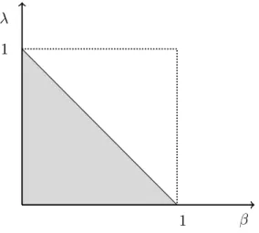
2 [(4β−7)λ2−4(β−2)2λ+ (β−2)3+λ3]< 1 2−β This inequality holds whenever:
λ <1−β
This result is depicted on Figure 5.1. The shaded area corresponds to the cases when anchoring yields lower average prices.
λ 1
1 β
Figure 5.1: Change of average prices.
Remark 2 Notice, that the output-weighted average price is even lower than the average price, since with anchoring the second period equilibrium prices are lower and the equilibrium quantities are greater than in the rst period.
The intuition behind the above result is that in the rst period, rms are increasing prices in order to create a favourable anchor for the sec- ond period where they can make up for the lost sales. However, prices in a Bertrand setup are strategic complements, hence when demands are more interrelated, this leads to a more signicant price increase in the rst period. Of course this implies that the rms are also able to charge a higher price in the second period as well. Therefore the average price in- creases if the products are close substitutes and decreases when demands are relatively independent of each other.
5.2.2 The general case
In this section we consider a more general case withn≥2rms playing an innite horizon game. In this case rms aim to maximise their dis-
counted prots of Πi =
P∞
t=1δt−1pi,tDi,t(pt, rt), withδ∈(0,1). Therefore, the respective Bell- man equations for this problem can be given as:
Vi,t(pi,t−1) = max
pi,t
pi,t
1−pi,t+X
j6=i
βpj,t+λ(pr,t−pi,t)
+ +δVi,t+1(pi,t)
for everyi, j= 1,2, . . . , n(j6=i), wherepr,t=
Pn ipi,t−1
n . Dropping time subscripts from the value function,sVi,t(pi,t−1), these simplify to:
Vi(pi) = max
pi
pi
1−pi+X
j6=i
βpj+λ(pr−pi)
+δVi(pi)
Let us assume thatVi(pi) =A+Bpi+Cp2i. In this case rst-order conditions yield:
1−pi+X
j6=i
βpj+λ P
j6=ipj−(n−1)pi
n
!
+ +pi
−1−(n−1)
n λ
+δB+ 2δCpi= 0
for everyi= 1,2, . . . , n. Imposing symmetry we have that:
p∗i = 1 +δB
2−(n−1)β+(n−1)n λ−2δC
for everyi= 1,2, . . . , n. For thisp∗i the Bellman equation simplies to:
A+Bp∗i +Cp∗i 2=p∗i
1−p∗i +X
j6=i
βp∗i
+δ
A+Bp∗i +Cp∗i 2
or
(1−δ)(A+Bp∗i +Cp∗i
2) =p∗i −[1−(n−1)β]p∗i 2
From this we have that:
A= 0 B= 1
1−δ C=−1−(n−1)β 1−δ Plugging these into our previous equation yields:
p∗i = 1
2−(1 +δ)(n−1)β+ (1−δ)(n−1)n λ
Solving the no-anchoring case fornrms we have that rms choose p∗∗i,t = 2−(n−1)β1 . Comparing this to the prices given by the previous equation we can show that:
Proposition 5.2 Price anchoring yields lower prices ifλ >1−δβδn . Proof: Let us dene∆p≡p∗i−p∗∗i = δ(n−1)β−(1−δ)n−1n λ
[2−(1+δ)(n−1)β+(1−δ)(n−1)
n λ][2−(n−1)β]. We shall prove that∆p<0. Since the denominator in∆pis positive we need that:
δ(n−1)β−(1−δ)n−1 n λ <0 This implies that:
λ > βδn 1−δ
Proposition 5.3 Price anchoring yields lower prots if and only if it yields lower prices.
Proof: Plugging the equilibrium prices into the respective prot func- tions we have that in the case of anchoring prots are:
πi∗= 1−δ(n−1)β+ (1−δ)(n−1)n λ [2−(1 +δ)(n−1)β+ (1−δ)(n−1)n λ]2 and without anchoring they equal to
π∗∗i = 1 [2−(n−1)β]2
for eachi= 1,2, . . . , n. Let∆π≡π∗i −π∗∗i . This is negative if:
[2−(n−1)β]2[1−δ(n−1)β+ (1−δ)(n−1) n λ]<
<[2−(1 +δ)(n−1)β+ (1−δ)(n−1) n λ]2 or
−[(1−δ)λ−βδn][(1−δ)λ+β(2−δ−β(n−1))n]<0 which simplies to:
λ > βδn 1−δ
Notice that this condition is the same as the one derived in the previous
proposition.
It is quite interesting that this time we obtain a lower bound forλ, opposite to our result in the two-period game. The explanation lies in the fact that the steady-state incentives are somewhat dierent than the ones that exist in a dynamic pricing game. The rms are not setting prices in order to exploit the anchor in the future. Rather the existence the anchoring in some sense pushes down the price limit in this Bertrand competition, since a stronger anchoring eect makes it more protable to decrease prices further.
Proposition 5.4 The price decreasing eect of anchoring is more ap- parent if fewer rms are active in the market. The same applies if rms produce highly dierentiated products (i.e. β→0) or if rms value future earnings less (i.e. δ→0)
Proof: The proof follows trivially from the previous proposition since the right-hand side of the inequality condition is increasing inn,β and
δ, respectively.
If there are fewer rms in the market, one rm can inuence the average price more, hence they have a larger incentive to lower their prices. If the products are more dierentiated, the rms own demand is less aected by the price decreases of the other rms, therefore there is more room to decrease prices. If the rms value future earnings less, then they are willing to lower prices more even when this does not lead to future gains.
5.3 Conclusion
Previous literature warns us that in certain cases rms are able to exploit consumer bias to increase their prots, while harming their consumers.
Anchoring is well-known and well-researched bias for psychologists as well as marketing professionals. Little research was done however on the issue how price anchoring aects the conclusions of our market models.
To at least partially answer this question, we investigated these eects within a nite horizon Bertrand game with dierentiated products. We assumed that the average price of the previous period serves as an anchor for the consumers, furthermore we assumed that this fact is common knowledge for the rms. Solving our model, we nd that in the case of anchoring, the consumer bias might lead to lower prices. Somewhat surprisingly, we also nd that this price-lowering eect is more likely in more dierentiated markets, thus rms with higher market power are even less likely to exploit anchoring. In our more general innite-horizon model, we have further found that if there are less rms in an industry, it is more likely that price anchoring will lead to lower prices, also pointing in this direction. Even though the eects of anchoring on equilibrium oligopoly prices is ambiguous, we have shown that it can lead to lower prices, especially in those cases when the rms have higher market power.
Adaval, R. and Wyer Jr, R. S. (2011). Conscious and nonconscious com- parisons with price anchors: Eects on willingness to pay for related and unrelated products, Journal of Marketing Research, 48(2), 355- 365.
Amir, O., Ariely, D. and Carmon, Z. (2008), The dissociation between monetary assessment and predicted utility, Marketing Science, 27(6), 1055-1064.
Ariely, D., Loewenstein, G. and Prelec, D. (2003), "Coherent Arbitrari- ness": Stable Demand Curves Without Stable Preferences, The Quar- terly Journal of Economics, 118(1), 73-105.
Arijit, M. (2010), Price discrimination in oligopoly with asymmetric rms, Economics Bulletin 30, 2668-2670.
Asch, B. (1990), Do incentives matter? The case of Navy recruiters, Industrial & Labor Relations Review, 43(3), 89-106.
d'Aspremont, C., Gabszewicz, J. J. and Thisse, J. F. (1979), On Hotelling's "Stability in Competition", Econometrica, 47(5), 1145- 1150.
Basu, K. (1995), Stackelberg equilibrium in oligopoly: an explanation based on managerial incentives, Economics Letters, 49(4), 459-464.
Basu, K. and Kalyanaram, G. (1990), On the relative performance of linear versus nonlinear compensation plans, International Journal of Research in Marketing, 7(3), 171-178.
Baucells, M., Weber, M. and Welfens, F. (2011), Reference-point forma- tion and updating, Management Science, 57(3), 506-519.