Price vs. Quantity in Oligopoly Games
Attila Tasn´adi
Department of Mathematics, Corvinus University of Budapest, H-1093 Budapest, F˝ov´am t´er 8, Hungary∗
July 29, 2005.
Appeared in theInternational Journal of Industrial Organization†, 24(2006), 541-554, cElsevier Science S.A.
Abstract: Price-setting and quantity-setting oligopoly games lead to extremely different outcomes in the market. One natural way to ad- dress this problem is to formulate a model in which some firms use price while the remaining firms use quantity as their decision variable.
We introduce a mixed oligopoly game of this type and determine its equilibria. In addition, we consider an extension of this mixed oligopoly game through which the choice of the decision variables can be endo- genized. We prove the emergence of the Cournot game.
JEL Classification Number: D43; L13.
Keywords: Cournot, Bertrand-Edgeworth, Oligopoly.
1 Introduction
The literature on oligopoly theory distinguishes between two main classes of models depending on whether price or quantity is regarded as the decision variable. Since these two types of models lead to extremely different outcomes in the market, one would like to consider an intermediate model in which some firms quote prices while others ‘dump’ quantities. Such kinds of models have been formulated in the homogeneous good framework by Allen (1992) and by Qin and Stuart (1997), and in the heterogeneous good framework by Singh and Vives (1984), Klemperer and Meyer (1986), Szidarovszky and Moln´ar (1992) and Tanaka (2001a, 2001b). For economically relevant examples in which the firms are able to choose their decision variables (price or quantity) we refer to Klemperer and Meyer (1986, Section 2).
∗Telephone/fax: (+36 1) 3870834, E-mail: attila.tasnadi@uni-corvinus.hu
†IJIO at sciencedirect
We consider homogeneous good oligopoly markets. Allen (1992) intro- duced a duopoly game in which the decision variable of one firm was its quantity while that of the other firm was its price, and determined the Nash equilibrium under various orders of moves. Qin and Stuart (1997) formulated a mixed oligopoly game in which some firms set their quantities and the re- maining firms set their prices. They showed that if the firms are allowed to choose between price-setting and quantity-setting behavior, then both the Bertrand and the Cournot outcome could emerge.
One can say that the above mentioned previous works crossed the Cournot model with the Bertrand model. Our analysis is of a similar nature, but we regard a Bertrand-Edgeworth price-setting game instead of the simpler Bertrand price-setting game because in many cases we cannot force the price- setting firms to satisfy the entire demand they face, especially, when they are not able to do this due to capacity constraints or when they could earn more profits by serving fewer consumers. The Bertrand-Edgeworth game does not have an equilibrium in pure strategies for many cost functions and therefore, in order to keep our analysis tractable we will assume that the firms have constant and identical unit costs up to a uniform capacity constraint.
We prove that for small capacities our mixed model possesses a Nash equilibrium in pure strategies, which in fact equals both the Bertrand and the Cournot solutions (Proposition 1). In the more intriguing case of larger capacities we demonstrate the non-existence of Nash equilibrium in pure strategies if there are at least two price-setting firms (Corollary 1). For this case we determine the ‘symmetric’ mixed-strategy equilibrium of the game.
Our mixed model turns out to be a ‘consistent’ extension of price-setting and quantity-setting games, since the equilibrium price distribution decreases (in the sense of first order stochastic dominance) if any firm switches from being a quantity player to being a price player (Theorem 2). If we extend our mixed oligopoly model by allowing the firms to select their decision variables, then we find that in any case the Cournot game arises as the equilibrium of the extended game. In this respect our result is always deterministic, in contrast to Qin and Stuart’s (1997) Theorem 1, in which multiple equilibria may arise.
The remainder of the paper is organized as follows. In Section 2 we present our mixed oligopoly model. In Sections 3 and 4 we assume that the firms’
decision variables are predetermined and we calculate in these two Sections the pure-strategy and the ‘symmetric’ mixed-strategy equilibria, respectively.
In Section 5 we endogenize the choice of decision variables and Section 6 concludes our paper. The more technical proof of Proposition 3 can be found in the Appendix.
2 The model
Suppose that there are n firms in the market. We assume that the firms have zero fixed costs and constant marginal costs up to some positive and identical capacity constraint k. In particular, we require that the firms have identical capacity constraints to keep our analysis tractable, since the cal- culation of the non-degenerated mixed-strategy equilibrium of the Bertrand- Edgeworth oligopoly game is a difficult task. Vives (1986) determined the symmetric mixed-strategy equilibrium of the symmetric Bertrand-Edgeworth game with capacity constraints. However, for the case of asymmetric capaci- ties the problem has not yet been solved. A step in this direction was done by Gangopadhyay (1993), who could determine at least the equilibrium profit of the firm with the largest capacity and could also provide boundary values for the equilibrium profits of the other firms.
We impose the commonly applied zero marginal cost assumption.1 The assumptions imposed on the oligopolists’ cost functions and on the demand curve are summarized below.
Assumption 1. There are n oligopolists in the market with zero unit costs and identical capacity constraints k >0.
Assumption 2. D : R+ → R+ is strictly decreasing on [0, b], identically zero on [b,∞), continuous at b, twice continuously differentiable on (0, b) and concave on [0, b].
Clearly, any price-setting firm will not set its price above b. We write a for the horizontal intercept; i.e., D(0) =a. Moreover, let us denote byP the inverse demand function. Thus, P (q) = D−1(q) for 0 < q ≤ a, P (0) = b, and P (q) = 0 for q > a.
We define pc to be the price which clears the firms’ aggregate capacity from the market if such a price exists, and zero otherwise. That is, pc = P (nk). We will refer to this price as the market-clearing price. We shall denote by Dr(p) := (D(p)−(n−1)k)+ the residual demand curve and its inverse by Pr(q). It can be easily verified that Pr(q) =P (q+ (n−1)k).
Assuming efficient rationing, the functionπr(p) :=pDr(p) will equal a firm’s profit whenever it sets the highest price in the pure price-setting game and p ≥ pc. We ensure that every firm will be active in the market by the next assumption.
Assumption 3. (n−1)k < a.
1For a paper focusing on cost asymmetry in a Bertrand-Edgeworth duopoly game we refer to Deneckere and Kovenock (1996).
Let p := arg maxp∈[0,b]πr(p) and π := πr(p). Clearly, pc and p are well defined whenever Assumptions 1-3 are satisfied. Note that Assumption 3 also ensures that p >0 and π >0.
We denote byN ={1, . . . , n} the set of firms, by I ⊂N the set of price- setting firms and byJ =N\I the set of quantity-setting firms. Letpi ∈[0, b]
be the price decision of firm i ∈I and qj ∈[0, k] be the quantity decision of firmj ∈J. Hence, the price decisions and the quantity decisions are contained in vectors p∈[0, b]nand q∈[0, k]n, respectively. Note that the values for pj and qi are without meaning for any quantity-setting firm j ∈ J and for any price-setting firm i∈I, respectively. For fixed decisions (p,q) the aggregate supply of the firms at price p is given by Sp,q(p) := P
j∈Jqj +P
i∈I,pi≤pk.
We have to specify a demand-allocating mechanism and the price of the quantity-setting firms’ product as a function of the price and quantity actions taken by the firms. We define the quantity-setting firms’ sales price, denoted by p∗(p,q), to be the lowest price at which the demand is less or equal to the aggregate supply of the firms. Formally, p∗(p,q) :=
inf{p∈[0, b]|D(p)≤Sp,q(p)}= min{p∈[0, b]|D(p)≤Sp,q(p)}. We can write min instead of inf because D(p)−Sp,q(p) is a decreasing and right-continuous function in p. Observe that p∗(p,q) is even defined for the purely price-setting game.
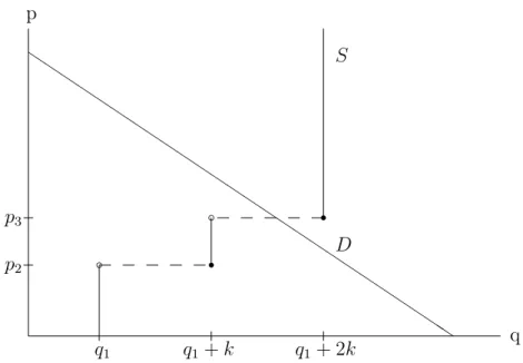
At price levelp∗(p,q) aggregate supply may exceed market demand. This case is illustrated in Figure 1 in which there are two price-setting firms and one quantity-setting firm. In the situation presented in Figure 1 the sales price for the quantity-setting firm’s product equals p3. In case of price ties, we as- sume for simplicity, that the demand is allocated first to the quantity-setting firms and afterwards the remaining demand is shared by the price-setting firms in proportion of their capacities. The first part of this assumption, i.e.
that the demand is allocated first to the quantity-setting firms, expresses our intuition that price setters shall face quantity adjustment, while quantity setters shall face price adjustment. The demand satisfied by firm j ∈ J is given by
∆j(p,q) :=
( qj if p∗(p,q)>0, minn
qj,Pqj
l∈JqlD(0)o
if p∗(p,q) = 0;
and therefore, its profit equalsπj(p,q) = p∗(p,q)qj. We define the demand satisfied by a price-setting firm i∈I by
∆i(p,q) :=
0 if pi > p∗(p,q),
1 v
D(pi)−P
j∈Jqj−uk
if pi =p∗(p,q),
k if pi < p∗(p,q),
p
q
Q Q
Q Q
Q Q
Q Q
Q Q
Q Q
Q Q
Q Q
Q Q
Q Q
Q Q
Q Q
S
D p2
p3
b
q1
r b
q1+k
r
q1+ 2k
Figure 1: Quantity-setting firms product price
where u denotes the number of price-setting firms who set price lower than pi and v denotes the number of price-setting firms who set price pi. Thus, firm i ∈ I makes πi(p,q) := pi∆i(p,q) profit. We shall denote by OI the mixed oligopoly game we have just defined.
3 Equilibrium in pure strategies
Now, we turn to the investigation of the mixed oligopoly game OI. In this Section we determine those conditions under which an equilibrium in pure strategies exists. If such an equilibrium exists, then we show that it is unique.
In two cases the outcome of game OI is well-known: for I = ∅ and I = N. In the first case our mixed model reduces to the Cournot game, while in the second case to the Bertrand-Edgeworth game.
We will proceed step by step in order to obtain a better understanding of the equilibrium behavior of the mixed oligopoly game. The following Lemma states that in a pure-strategy equilibrium the price-setting firms must set the same prices.
Lemma 1. Under Assumptions 1-3, if (p,q) is a pure-strategy equilibrium, then pi =pj for any i, j ∈I.
Proof. The statement is obviously true if |I| ≤ 1. Thus, we have only to consider the case of |I|>1. Let firmj be one of the firms setting the lowest
price; that is, pj ≤ pi for all i ∈ I. Suppose that pj < pi holds for a firm i ∈ I. If ∆i(p,q) > 0, then firm j can increase its profit by setting its price arbitrarily close to but below pi. If ∆i(p,q) = 0, then πi(p,q) = 0.
But firm i can make positive profit, for instance, by switching its price to P 12((n−1)k+a)
so that it faces a demand of at least 12(a−(n−1)k) because of Assumption 3. Thus, firm iwould deviate, and therefore, pj < pi cannot be the case.
Next, we prove that in a pure-strategy equilibrium every price-setting firm’s price must be equal to the sales price of the quantity-setting firms.
Lemma 2. Let |J|>0 and Assumptions 1-3 be satisfied. If(p,q) is a pure- strategy equilibrium, then pi =p∗(p,q) for any i∈I.
Proof. Clearly, the Lemma holds if |I| = 0. Therefore, in what follows we can assume that |I| > 0. Suppose that pi 6=p∗(p,q) for some i ∈ I. Recall that any firmi∈I setting its price belowp∗(p,q) can sell its entire capacity.
Moreover, observe thatp∗(p,q) will not change if prices lower thanp∗(p,q) change as long as they remain lower than p∗(p,q). Thus, if pi < p∗(p,q), firm i can increase its profit by setting a price slightly below p∗(p,q), since it is still selling k but at a higher price. Ifpi > p∗(p,q), then firmi does not sell anything and makes zero profit. But firm ican achieve positive profit by making a sufficiently large price reduction because of Assumption 3.
Furthermore, if there is at least one price-setting firm in the market, then in a pure-strategy equilibrium the quantity-setting firms produce at their capacity limits.
Lemma 3. If |J| > 0, |I| > 0 and Assumptions 1-3 are satisfied, then we must have qj =k for all j ∈J in any pure-strategy equilibrium.
Proof. From Lemma 2 we know that in a pure-strategy equilibrium pi = p∗(p,q) must hold for alli∈I. Moreover, every firm’s profit must be positive because of Assumption 3, which implies ∆i(p,q) > 0. If qj < k, then firm j ∈J can increase its profit by an increase in its output, because this will not lead to a decrease ofp∗(p,q), since the increase in the output of the quantity- setting firm j will just result in a decrease of sales for the price-setting firms;
a contradiction.
Our next lemma establishes that in the presence of at least two price- setting firms a pure-strategy equilibrium requires the price-setting firms to sell at their capacity limits and that the prices all equal the market-clearing price.
Lemma 4. Suppose that |I| ≥ 2 and that Assumptions 1-3 are satisfied.
Then a pure-strategy equilibrium exists if and only if p ≤ pc. In addition, if a pure-strategy equilibrium exists, then it is given by qj =k for all j ∈J and pi =pc for all i∈I.
Proof. First, we show that if a pure-strategy equilibrium exists, then it is given by qj =k for all j ∈J and pi =pc for all i∈I. Suppose that|J|= 0.2 From Lemma 1 we know that in a possible equilibrium every firm sets the same price. But, if that price level exceedspc, then their sales will be less than their capacity level and therefore any of them can gain from undercutting its opponents. Now, we consider case |J| > 0. We have already shown in Lemma 3 that qj =k for all j ∈J. Furthermore, by Lemma 2 we must have pi =p∗(p,q) for any i∈I. Hence, pc ≤p∗(p,q). But if pc < p∗(p,q), then any price-setting firm i will sell less than k. Therefore, by just unilaterally undercutting the price p∗(p,q), any price-setting firm can increase its sales radically and thus increase its profit.
Second, we demonstrate the necessary and sufficient condition for the ex- istence of a pure-strategy equilibrium. If p≤pc, then it can be easily verified that qj = k for all j ∈ J and pi = pc for all i∈ I is an equilibrium in pure strategies. In particular, neither could a quantity-setting firm benefit from producing less thank nor could a price-setting firm benefit from changing its price. Moreover, if p > pc, then qj =k for all j ∈J and pi =pc for alli ∈I cannot be an equilibrium in pure strategies, since a price-setting firm could gain from switching to price p.
We shall denote by qm the unique revenue maximizing output on the inverse residual demand curvePr; i.e.,qm := arg maxq∈[0,a]qPr(q). Of course, qm =Dr(p). If k≤qm, then we will say that the firms havescarce capacity, while otherwise we will say that the firms have sufficient capacity. Note that a firm with scarce capacity will be eager to produce at its capacity limit. It can be verified that condition k ≤qm is equivalent topc≥p.
In the following proposition we establish that if the firms have scarce capacity, then there exists a unique pure-strategy equilibrium in any mixed oligopoly game.
Proposition 1. Under Assumptions 1-3, if the firms have scarce capacity, there exists a unique equilibrium in pure strategies in which the prices equal the market-clearing price and all firms produce at their capacity limits.
Proof. It can be easily verified that pi = pc for all i ∈ I and qj = k for all j ∈J is indeed a pure-strategy equilibrium of OI for any I ⊂N, because of
2This part is standard, since|J|= 0 is the pure price-setting case.
k ≤qm. In case of|I|= 0 uniqueness follows from Vives’s (1999) Theorm 2.8.
ForI ={i}uniqueness can be guaranteed by Lemma 3 and by the definition of p. Finally, if |I| ≥2, then Lemma 4 assures uniqueness.
We have to mention that this proposition and the next corollary is very similar to some results obtained by Kreps and Scheinkman (1983), Deneckere and Kovenock (1992) and Boccard and Wauthy (2000) for the purely price- setting game.
Corollary 1. Under Assumptions 1-3, if |I| ≥2, then OI has an equilibrium in pure strategies if and only if the firms have scarce capacity.
Let us denote by p the price for which pk = pDr(p). Suppose that the firms have sufficient capacity (implying p < p), then any firm is indifferent to satisfying residual demand at price level p or selling its entire capacity at the lower price level p.
Next, we investigate the case of only one price-setting firm. Because of Proposition 1 we can restrict ourselves to the case in which the firms have sufficient capacity.
Proposition 2. Suppose that the firms have sufficient capacity and that there is only one price-setting firm; i.e., I = {i} ⊂ N. Then under Assumptions 1-3 there exists a unique pure-strategy equilibrium, which is given by
∀j ∈J =N\ {i}:qj =k and pi =p= arg max
p∈[0,b]pDr(p). (1) Proof. First, we verify that the strategy profile given by equation (1) is an equilibrium. Clearly, a quantity-setting firm cannot increase its output be- yond its capacity level. A unilateral output decrease of at most k−qm will not change the sales price for the quantity-setting firms’ product, only in- crease the price-setting firm’s sales. If firmj reduces its output by more than k−qm, then the sales price for the quantity-setting firms’ product will equal to Pr(qj + (n−1)k). Thus, a unilateral output decrease by any firm j ∈ J will inevitably lead to a decrease in its own profit level because qj < qm. It is obvious that firm i will not deviate from price p. Hence, equation (1) determines a pure-strategy equilibrium profile, which is even unique because of Lemmas 2 and 3.
We have to emphasize that by Proposition 2 a mixed oligopoly gameO{i}
with a price-setting firm having sufficient capacity yields an implementation of Forcheimer’s dominant firm model of price leadership (see Deneckere and Kovenock, 1992), because the price-setting firm sets its price by maximizing
profit with respect to its residual demand curve and the sales price for the remaining firms’ product equals that price.
We still have to consider the Cournot game; that is, the case in which every firm behaves as a quantity setter. The existence of a pure-strategy equilibrium in the Cournot game has been investigated extensively in the lit- erature (see, for instance, Szidarovszky and Yakowitz, 1977; Novshek, 1985;
Amir, 1996). If every firm behaves as a quantity-setter, then under Assump- tions 1-3 the existence of a unique equilibrium in pure strategies can be easily verified by applying Vives’s (1999) Theorem 2.8. By Vives’s (1999) Remark 17 it follows even that this unique equilibrium has to be a symmetric one.
The next theorem summarizes our results concerning the pure-strategy equilibrium of game OI.
Theorem 1. Under Assumptions 1-3 the following statements hold true con- cerning the mixed oligopoly game OI.
1. If qm ≥k, then there is a unique equilibrium in pure strategies in which the prices equal the market-clearing price and all firms produce at their capacity limits.
2. If qm < k and I ={i}, then the equilibrium in pure strategies results in a model of dominant firm price leadership, with the price-setting firm as leader.
3. If qm < k and I =∅, then the Cournot solution is the unique equilib- rium in pure strategies.
4. In any other case a pure-strategy equilibrium does not exist.
4 Equilibrium in mixed strategies
In this section we consider the case in which we have a non-existence of equilibrium in pure strategies; that is, the case of sufficient capacities. To de- termine the mixed-strategy equilibrium is a difficult task even for the purely price-setting game. Vives (1986) determined the symmetric mixed-strategy equilibrium for the symmetric Bertrand-Edgeworth game. Here we will also restrict ourselves to ‘symmetric’ mixed-strategy equilibria, though we do not have a symmetric game and therefore, we introduce the notion of a quasi- symmetric equilibrium.
Definition 1. We say that a strategy profile (p,q) is a quasi-symmetric equilibrium of the oligopoly game OI if (p,q) is an equilibrium of the game OI, pi =pj for all i, j ∈I and qi =qj for all i, j ∈J.
The notion of quasi-symmetric equilibrium can be defined for pure strate- gies and for mixed strategies as well.
Our first Proposition for the case of sufficient capacities gives us the unique quasi-symmetric equilibrium in mixed strategies.
Proposition 3. Suppose that Assumptions 1-3 are satisfied, the firms in OI have sufficient capacities (qm < k) and there are at least two price-setting firms (|I| ≥ 2). Then there exists a unique quasi-symmetric equilibrium in mixed strategies in which each price-setting firm randomizes according to the following atomless distribution function
F|I|(p) =
0, if p∈[0, p),
k−π/p nk−D(p)
|I|−11
, if p∈[p, p],
1, if p∈(p, b],
(2)
and each quantity-setting firm produces k with probability one. In addition, the quantity-setting firms’ sales prices are distributed according to the distri- bution function
G|I|(p) =
0, if p∈[0, p),
k−π/p
nk−D(p)
|I|−1|I|
, if p∈[p, p],
1, if p∈(p, b].
(3)
The proof of Proposition 3 is provided in the Appendix.
Our intuition suggests that given a fixed numbernof oligopolists the more price-setting firms we have the lower should be the prices in the market. The following theorem establishes that our extension of purely quantity-setting games and purely price-setting games is consistent with our intuition.
Theorem 2. Suppose that Assumptions 1-3 are satisfied, the firms have suffi- cient capacities (qm < k) and that the quasi-symmetric equilibrium is played.
Then in the sense of first-order stochastic dominance we have lower prices in OI than in OI0 whenever |I|>|I0|.
Proof. We can assume without loss of generality thatI0 ={1, . . . , i}andI = {1, . . . , i, i+ 1} because the firms are playing their quasi-symmetric mixed- strategy equilibrium strategies. We separate our proof into three subcases.
First, suppose that I0 =∅ and I ={1}. In this case we have to compare the equilibrium price of the Cournot game with the equilibrium price of the price leadership game (Proposition 2). Both games possess a deterministic
outcome. Taking Assumption 2 and qm < k into consideration the price leadership price has to be lower than the Cournot price, since
D(p)−(n−1)k < D(p)−(n−1)qc, where qc stands for the unique Cournot outcome of game OI0.3
Second, suppose that i = 1. Thus, we will compare the price leadership price with the equilibrium price distributions of the game having two price- setting firms. In the price leadership game the equilibrium price equals p with probability one, while in the case of two price-setting firms the highest price set by the two firms could be p. However, the two price-setting firms set prices less than p with probability one.
Third, suppose thati∈ {2, . . . , n−1}. We start with considering a price- setting firm j ∈ {1, . . . , i}. Since
0< i−1 s
k−π/p nk−D(p)
< i s
k−π/p nk−D(p)
<1 for any p ∈ p, p
firm j has to set lower prices with higher probabilities in OI than in OI0. Now we consider a quantity-setting firm j ∈ {i+ 2, . . . , n}
(this case is vacuous if i=n−1). Applying equation (3), we obtain k−π/p
nk−D(p) i−1i
<
k−π/p nk−D(p)
i+1i
for anyp∈ p, p
because of 1< i+1i < i−1i . Finally, we have to consider firm i+ 1, which is a quantity setter in OI0 and a price setter in OI. Comparing equation (3) for i price-setting firms with equation (2) for i+ 1 price-setting firms we get
k−π/p nk−D(p)
i−1i
<
k−π/p nk−D(p)
1i
for any p∈ p, p .
5 Endogenous choice of roles
In the previous sections we investigated the equilibrium behavior of a mixed oligopoly game in which the strategic variables of the firms were predeter- mined and made some comparisons. Now, we turn to the question what
3It can be verified thatqm< kimpliesqc< k.
happens if the firms are able to select whether they behave in a Cournot-like manner or in a Bertrand-Edgeworth-like manner. We tackle this topic in the following way: Consider an extension of game OI in which, first, the firms simultaneously select their decision variables and, second, they determine simultaneously the magnitude of their decision variables.
We shall denote by C and BE whether a firm uses quantity or price as its decision variable. Let V = {C, BE}. Then the decisions of firm i ∈ N is denoted by s = (v, x) ∈ V ×R+, where v describes the selected decision variable and x denotes the selected price or quantity.
Theorem 3. Let Assumptions 1-3 be fulfilled and suppose that in case of sufficient capacities (qm < k) the quasi-symmetric equilibrium is played. Then the above game has the following subgame-perfect Nash equilibria.
1. If qm ≥k, every oligopoly game OI could arise in equilibrium. Particu- larly, each firm is indifferent to whether being a price setter with actions (BE, pc) or being a quantity setter with actions (C, k)regardless of the other firms’ actions.
2. If qm < k, then only the Cournot game could emerge, that is, the equi- librium actions of firm i are(C, qc) for alli∈N, where qc denotes the unique Cournot output.
Proof. Point 1 of Theorem 1 implies point 1. Thus, we have only to establish point 2. We show that choosing quantity as the decision variable strictly dominates choosing price in stage one. Observe that the price-setting firms achieve π =pk profits in any oligopoly game OI.
First, consider the case in which there are at least two price-setting firms.
Now if a price-setting firm unilaterally switches to become a quantity setter, then it can sell with probability one its entire capacity at higher prices than p. Hence, it clearly benefits from choosing C in stage one instead of choosing BE.
Second, consider the case in which we have just one price-setting firm.
Then the price leader’s profit equals π =πr(p) =pk, while if it switches to being a quantity setter, then it will face a more favorable demand D(p)− (n−1)qc, where qc stands for the unique Cournot outcome.4 Hence, it can gain from selecting C instead ofBE.
4See also the second paragraph of the proof of Theorem 2.
6 Concluding remarks
Considering the symmetric Bertrand-Edgeworth game, like in Vives (1986), scarce capacity is usually referred to as small capacity, while sufficient ca- pacity as intermediate capacity. There is also a third case of large capacities, which we omitted in our analysis by imposing Assumption 3. For the case of (n−1)k ≥ a it can be verified that for all pure-strategy equilibria we must have p∗(p,q) = 0 if there is at least one price-setting firm in the market. A profile (p,q) is an equilibrium if the demand at price 0 can even be satisfied when one firm with positive supply at price 0 leaves the market. It can be also checked that the ‘traditional’ Cournot outcome is another solution of the pure quantity-setting game besides the above mentioned type of equilibria.
It is worth mentioning that in case of k ≥ a we obtain the same payoff functions as Qin and Stuart (1997). However, in their paper a firm simulta- neously chooses its decision variable and its magnitude, while in our paper this choice happens sequentially.
A possible extension would be to allow for asymmetric capacities. This extension would not alter the validity of Lemmas 1-4, and Proposition 1.
However, firms with too small capacities cannot become a price leader, since in a profile specified according to Proposition 2 the firm with the largest ca- pacity might have the incentive either to increase its price or to decrease its quantity. This observation also imposes a slight restriction on the extension of Theorem 1. In what follows assume that the firms’ capacity constraints ki are ordered decreasingly. Consider profiles in which all quantity-setting firms produce kj with probability one and the price-setting firms’ mixed strategies are determined by a mixed-strategy equilibrium of a Bertrand- Edgeworth game with demand curve D(p)−P
j∈Jkj. These profiles con- stitute for any |I| ≥ 2 and I ⊂ {1, . . . , n} a mixed-strategy equilibrium of game OI if the capacities are not ‘too asymmetric’. In particular, the capac- ities are too asymmetric if the largest-capacity firm makes a profit less than maxp1∈[0,b]p1(D(p1)−Pn
m=2km)+ in the above specified equilibrium of the game O{n−1,n}. Thus, one might expect that Theorems 2 and 3 can be gener- alized for the case of not too asymmetric capacities. However, it appears to be difficult to give an explicit condition for capacities being too asymmetric.
Acknowledgements
I am grateful to Dan Kovenock and two anonymous referees for many com- ments and suggestions that led to substantial improvements in the paper.
This research was done during the author’s Bolyai J´anos Research Fellow-
ship provided by the Hungarian Academy of Sciences (MTA).
Appendix
Proof of Proposition 3. We can assume without loss of generality that I = {1, . . . , i}. Letj :=n−i. Our proof will be by construction. Pick an arbitrary quasi-symmetric equilibrium with strategies F and G played by the price- setting and quantity-setting firms, respectively. Let [p,e bp] be the support of F and [eq,q] be the support ofb G, that is, pe = sup{p∈[0, b]|F(p) = 0}, pb = inf{p∈[0, b]|F(p) = 1}, qe = sup{q∈[0, a]|G(q) = 0} and qb = inf{q∈[0, a]|G(q) = 1}.5 Observe thatpe≥p.
Step 1:We show that F is atomless on (ep,p] and ifb F has an atom atp,e then D(p) =e ik+jq.b
Suppose thatF has an atom at pricep∈[p,e p] and letb αdenote the mass at price p. Then all price-setting firms set price p with probability αi > 0.
We separate our argument into three cases.
(i) If ik+jq > D(p), then the price-setting firms cannot sell their entireb capacity with probability one when they all set price p. Hence, there exists a sufficiently small ε >0 so that a price-setting firm can increase its profit by unilaterally shifting the mass α from price p to pricep−ε; a contradiction.
(ii) If ik +jq < D(p), then a price-setting firm can increase its profit byb setting a price slightly above p with probability one; a contradiction. (iii) If ik+jqb=D(p), then we must havep=ep.
We conclude thatF cannot have an atom at pin cases (i) and (ii). More- over, F can only have an atom in case (iii).
Step 2: We show that the quantity-setting firms play pure strategies in a quasi-symmetric equilibrium, that is, qe=bq.
We shall denote by u(p1, . . . , pi, Q−, q) the sales price of the quantity- setting firms when the price-setting firms set prices p1, . . . , pi, a quantity- setting firm produces q ∈[0, k] and all other quantity-setting firms together produce Q−∈[0,(j−1)k]. Note that uis continuous and decreasing inq for any givenp1, . . . , pi andQ−. In addition,uis twice continuously differentiable with the exception of at most two points in q∈[0, k]. Moreover, if ∂q∂u does not exist at q0 ≤ q00 ∈ [0, k], then ∂q∂u is concave on [0, q0), (q0, q00) and (q00, k]. Let G− =G∗ · · · ∗G denote the distribution function of Q− and let h(q) := R
u(p1, . . . , pi, Q−, q)dF . . . dF dG− denote the profit of a quantity- setting firm producing q if the other firms are playing their quasi-symmetric equilibrium strategies F and G.
5We follow the convention that the distribution functions are left continuous.
For any givenp1, . . . , pi andQ−we can construct a sequence of decreasing twice continuously differentiable functions (um)∞m=1 converging uniformly to u from below such that u(q)−um(q) < 1/m for all q ∈ [0, k] and that the graph of u0m is identical to the graph of u0 with the exception of a union of at most two disjoint squares of shapes (q0 −δm0 , q0+δm0 )×(pi0 −ε0m, pi0) or (q0, q0+δm0 )×(pi0−ε0m, pi0), where the graph ofu has a kink at point (q0, pi0) and δm0 , ε0m <1/m. The possible cases are illustrated in Figure 2.
k u um
q q0 q0+δm0 p
pi0
- 6
@
@
@
@
k u, um
q q0−δ0m q0+δ0m p
pi0
- 6
@
@
@
@
@@
k u um
q q0 q00
p pi0
pi00
- 6
@
@
@
@
Figure 2: The three types of kinks in [0, k].
Now we can define a sequence (hm)∞m=1 of perturbed payoff functions by hm(q) := qR
um(p1, . . . , pi, Q−, q)dF . . . dF dG− for all q ∈ [0, k]. It follows from standard results thathm converges uniformly from below tohand that h is continuous.
We show that hm has a unique maximum point in [q,eq] for sufficientlyb largemand several other useful properties of h0mand h00m. The first derivative of hm equals
h0m(q) = Z
A
um(p, Q−, q)dFdG−+q Z
A
∂
∂qum(p, Q−, q)dFdG−, (4) whereA:= [p,ep]bi×[(j −1)q,e (j −1)q],b p = (p1, . . . , pi) andF=F⊗ · · · ⊗F. It can be verified that the first part of the right-hand side of (4) is greater or equal than p. Therefore, hm strictly increases atq if
− Z
A
∂
∂qum(p, Q−, q)dFdG− < p
2k. (5)
If (5) is not satisfied, we will consider the second derivative of hm h00m(q) = 2
Z
A
∂
∂qum(p, Q−, q)dFdG−+q Z
A
∂2
∂q2um(p, Q−, q)dFdG−. (6) The first part of the right-hand side of (6) is smaller than or equal to −p/k if (5) is not satisfied. For any given (p, Q−)∈A the integrand of the second
part of the right-hand side of (6) can only be positive in at most two intervals, which are each contained in (q0−1/m, q0+1/m) or (q0, q0+1/m), whereq0 is a kink in [q,e bq]. Since this disturbing intervals are getting smaller asmincreases, it can verified that the probability that the sales price of the quantity-setting firms lies by at most 1/mbelow a ‘kink price’, tends to zero by Step 1. Thus, there exists an m0 such that
q Z
A
∂2
∂q2um(p, Q−, q)dFdG−< p 2k for all m > m0; and therefore,
h00m(q)<− p
2k (7)
must hold for a sufficiently large m. Observe that the bound in (7) is not a function of q.
To summarize, we have learned by investigating the first and second derivatives of hm that there exists an m0 such that for all m ≥ m0 we have that hm strictly increases by more than p/2 or hm will be strictly concave with a bound on concavity (7). This also implies for sufficiently largem that at a stationary point of hm in [q,e bq] we must have a local maximum. Hence, the set of maximum points of h cannot be disconnected since hm converges uniformly from below toh. In addition, the maximum pointqm ofhm in [eq,q]b has to be unique, since otherwise (7) would be violated.
Let [c, d]⊆[q,e bq] be the set of maximum points ofhin [q,eq]. Observe thatb the sequence qm has not only a cluster point but also a limit point because hm approaches h monotonically. We shall denote byq∗ the limit point of the sequence qm. Clearly, q∗ ∈[c, d].
Suppose that q∗ < d. Then qm < d for sufficiently large m. Since hm is strictly decreasing on (qm, d), (5) is violated in (qm, d). Therefore, we must have
hm(q)≤hm(qm)− p
4k (q−qm)2
by (7), which implies that limm→∞hm(d) < h(d); a contradiction. Thus, q∗ < dcannot be the case.
Assume thatq∗ =d. Then by an interplay of the conditions restrictingh0 and h00 we can derive that
hm(q)≤hm(qm)−min n p
4k (qm−q)2,p
2(qm−q) o
for all q ∈ [c, qm]. This would imply limm→∞hm(c) < h(c) if c < d, and therefore, it follows that c=d, which means that the quantity-setting firms have to play pure strategies in a quasi-symmetric equilibrium.
Step 3:We establish thatF cannot have an atom at pricep. Suppose thate F has an atom at price peand let us denote by q the pure strategies played by the quantity-setting firms. Then we must have D(p) =e ik+jq by Steps 1 and 2, which in turn implies that the sales price of the quantity-setting firms’ product equals the highest price set by a price-setting firm. Thus, if q < k, a quantity-setting firm could benefit from increasing its quantity.
Hence, we must have q = k. But then a price-setting firm could gain from setting a slightly lower price than pewith probability one instead of playing F; a contradiction.
Step 4:We determine the quasi-symmetric equilibrium strategyF of the price-setting firms given that every quantity-setting firm plays the same pure strategy q ∈[0, k] in a quasi-symmetric equilibrium.
From Steps 1 and 3 we know that in any quasi-symmetric equilib- rium the price-setting firms’ strategies are atomless. Thus, at price pb any price-setting firm can sell an amount of (D(p)b −(i−1)k−jq)+ with probability one. Hence, in an equilibrium we must have pb = pq :=
arg maxp∈[0,b]p(D(p)−(i−1)k−jq)+ and we write πq for the price-setting firms’ equilibrium profits. We shall denote byp
qthe price for whichp
qk =πq. The expected profits at price epequal epk=πq, and therefore, ep=p
q follows.
Thus, for all p∈[p
q, pq] we must have
[F(p)]i−1p(D(p)−(i−1)k−jq) +
1−[F(p)]i−1
pk =πq, from which we obtain through simple rearrangements
F(p) =
0 if p∈[0, p
q),
i−1
r
k−πq
p
ik+jq−D(p) if p∈[p
q, pq],
1 if p∈(pq, b].
(8)
Step 5: Given the behavior of the price-setting firms derived in Step 4 we cannot have a quasi-symmetric equilibrium with q < k, since then for all realizations of prices p1, . . . , pi a unilateral increase of a quantity- setting firm’s production would not decrease the quantity-setting firms’ sales price. Hence, we must have q = k in a quasi-symmetric equilibrium. Now by replacing q with k in equation (8) we obtain equation (2). Thus, if a quasi-symmetric equilibrium exists, then it is given by Proposition 3.
Step 6: We still have to check whether it is optimal for one quantity- setting firm to producekwhenever the price-setting firms are all playing their mixed strategiesF, given by equation (2), and all other quantity-setting firms produce k. Assume that p equals the quantity-setting firms’ sales prices in
a realization of the quasi-symmetric equilibrium stated in the Proposition.
Clearly, p ∈ p, p
. Changing firm j’s quantity from k to qj ∈ [Dr(p), k), does not change p, and therefore, reduces the profit of firmj ∈J. Moreover, for any quantityqj ∈[0, Dr(p)) we haveqjp < Dr(p)p≤Dr(p)p=kp≤kp and thus, a quantity-setting firm cannot gain from producing less than k.
Step 7:Finally, the quantity-setting firms’ sales prices have distribution function G, since the quantity-setting firms’ sales prices equal the highest price set by the price-setting firms. Thus, G(p) = [F(p)]i.
References
[1] Allen, B., 1992, Price and quantity competition in homogeneous markets, Economics Letters 38, 417-422.
[2] Amir, R., 1996, Cournot Oligopoly and the Theory of Supermodular Games, Games and Economic Behavior 15, 132-148.
[3] Boccard, N. and X. Wauthy, 2000, Bertrand competition and Cournot outcomes: further results, Economics Letters 68, 279-285.
[4] Deneckere, R. and D. Kovenock, 1992, Price Leadership, Review of Eco- nomic Studies 59, 143-162.
[5] Deneckere, R. and D. Kovenock, 1996, Bertrand-Edgeworth duopoly with unit cost asymmetry, Economic Theory 8, 1-25.
[6] Gangopadhyay, S., 1993, Simultaneous vs Sequential Move Price Games:
A comparison of equilibrium payoffs, Discussion Paper No. 93-01, Indian Statistical Institute.
[7] Klemperer, P. and M. Meyer, 1986, Price competition vs. quantity com- petition: the role of uncertainty, RAND Journal of Economics 17, 546-554.
[8] Kreps, D.M. and J.A. Scheinkman, 1983, Quantity precommitment and Bertrand competition yield Cournot outcomes, Bell Journal of Economics 14, 326-337.
[9] Novshek, W., 1985, On the Existence of Cournot Equilibrium, Review of Economic Studies 52, 85-98.
[10] Qin, C.-Z. and C. Stuart, 1997, Bertrand versus Cournot revisited. Eco- nomic Theory 10, 497-507.
[11] Singh, N. and X. Vives, 1984, Price and quantity competition in a dif- ferentiated duopoly, RAND Journal of Economics 15, 546-554.
[12] Szidarovszky, F. and S. Moln´ar, 1992, Bertrand, Cournot and Mixed Oligopolies, Keio Economic Studies 29, 1-7.
[13] Szidarovszky, F. and S. Yakowitz, 1977, A New Proof of the Existence and Uniqueness of the Cournot equilibrium, International Economic Re- view 18, 787-789.
[14] Tanaka, Y., 2001a, Profitability of price and quantity strategies in an oligopoly, Journal of Mathematical Economics 35, 409-418.
[15] Tanaka, Y., 2001b, Profitability of price and quantity strategies in a duopoly with vertical product differentiation, Economic Theory 17, 693- 700.
[16] Vives, X., 1986, Rationing Rules and Bertrand-Edgeworth Equilibria in Large Markets, Economics Letters 21, 113-116.
[17] Vives, X., 1999, Oligopoly Pricing: Old Ideas and New Tools (MIT Press, Cambridge MA).
![Figure 2: The three types of kinks in [0, k].](https://thumb-eu.123doks.com/thumbv2/9dokorg/949481.55034/15.892.157.725.363.539/figure-types-kinks-k.webp)
