A new perturbative solution to the motion around triangular Lagrangian points in the elliptic restricted three-body problem

(will be inserted by the editor)

A new perturbative solution to the motion around triangular Lagrangian points in the elliptic restricted three-body problem

B´alint Boldizs´ar · Tam´as Kov´acs · J´ozsef Vany´o

Received: date / Accepted: date

Abstract The equations of motion of planar elliptic restricted three body problem are transformed to four decoupled Hill’s equations. By using the Floquet theorem analytic solution to the oscillator equations with time dependent periodic coefficients are presented. We show that the new analytic approach is valid for system parameters 0<e≤0.05 and 0<µ≤0.01 whereedenotes the eccentricity of primaries whileµis the mass parameter, respectively. We also clarify the transformation details that provide the applicability of the method.

Keywords ERTBP·Hill’s Equation·Floquet theorem PACS 34D10·70F07·34A25

1 Introduction

In the era of exoplanets and specifically designed space missions, the co-orbital motion in the vicinity of the equilateral points L₄ andL₅became again the focus of attention. Since the seminal work of Szebe- hely [Szebehely(1967)] the orbits near the libration points have been discussed extensively by the com- munity. Analytic description of the Trojan-like resonant dynamics in the elliptic case of restricted three- body problem (ERTBP) is based mainly on averaged motion. rdi [Erdi(1977),Erdi(1978)] showed the per- turbation effects up to second order in Jupiter’s eccentricity, perihelion and ascending node precession by using a three-parameter expansion. Morais [Morais(2001)] considered an averaged disturbing poten- tial to describe the secular variation of the Trojans’ orbital elements in case of an oblate primary. Recently, [Robutel et al(2016)Robutel, Niederman, and Pousse] and [P´aez et al(2016)P´aez, Locatelli, and Efthymiopoulos]

B. Boldizs´ar

Institute of Physics, E¨otv¨os Iniversity, Budapest, Hungary E-mail: bolbalaa@caesar.elte.hu

T. Kov´acs

Institute of Physics, E¨otv¨os Iniversity, Budapest, Hungary E-mail: tkovacs@general.elte.hu

J. Vany´o

Department of Physics, Eszterhzy Kroly College, Eger, Hungary E-mail: vanyo.jozsef@uni-eszterhazy.hu

arXiv:2006.14940v1 [astro-ph.EP] 26 Jun 2020

investigated the co-orbital resonance based on Hamiltonian formalism whereby the fast angles had been av- eraged out. These latter analytical studies are also capable to locate higher-order resonances as well as very slow secular frequencies.

It has been demonstrated [Tschauner(1971),Erdi(1974),Meire(1981),Matas(1982)] that the coupled equa- tions of the ERTBP can be written in the form of independent ordinary differential equations with vari- able coefficients. The primary goal of these studies is to explore the stability map of eccentricity–mass parameter dated back to [Danby(1964)]. Interestingly, the analysis given by [Erdi(1977)] [Eq. (24)] and [Robutel et al(2016)Robutel, Niederman, and Pousse] [Eq. (56)] also terminates at a pendulum-like equa-

tion, however, they do not attempt to solve it by classical techniques such as Floquet theorem [Lichtenberg and Lieberman(1983)].

Here we propose a detailed derivation of Hill’s equations of ERTBP and make a comprehensive analysis of their applicability which is still out of literature. Furthermore, analytic expressions for the solution of Hill’s equations are given in the regime of moderate eccentricities and mass parameter with good agreement of numerical calculations.

2 Basic context

In this paper we mainly follow the notations used in e.g. [Tschauner(1971),Meire(1980),Meire(1982)]. Mo- tion around theL₄andL₅Lagrangian points is determined by the coupled differential equations [Szebehely(1967)]

x⁰⁰−2y⁰=rc₁x, (1)

y⁰⁰+2x⁰=rc₂y, (2)

where the notations are

r= 1

1+ecos(v), µ= m₂

m₁+m₂, g=3µ(1−µ) and ci=3

2(1+ (−1)ⁱp

1−g) (i=1,2). (3) Here⁰denotes the derivation with respect to the true anomalyv.

2.1 Hill’s equations

We will show, that Eqs. (1)-(2) with a suitable transformation can be rewritten to four decoupled second order differential equations. Let us introducey₁,y₂,y^∗₁,y^∗₂with the following transformation







 x y x⁰ y⁰









= 1212

P₁P₂







 y₁ y₂ y^∗₁ y^∗₂,









, (4)

where12is the 2-dimensional identity matrix, and furthermoreP₁andP₂are introduced as







 y⁰₁ y⁰₂ y^∗₁⁰ y^∗₂⁰









= P₁ 0

0 P₂







 y₁ y₂ y^∗₁ y^∗₂









(5)

relation stands. Let us use the temporary notations ˜x= (x,y), ˜y1= (y₁,y2)and ˜y2= (y^∗₁,y^∗₂). The elements ofP_i(i=1,2) matrices can be gained by using the following identities

x˜

˜ x⁰

= 1212

P₁P₂

˜ y₁

˜ y₂

=

y˜₁+y˜₂ P₁y˜₁+P₂y˜₂

, (6)

from which it simply follows, that x˜⁰

˜ x⁰⁰

=

y˜⁰₁+y˜⁰₂

P⁰₁y˜₁+P₁y˜⁰₁+P⁰₂y˜₂+P₂y˜⁰₂

=

0 12

rC2D

˜ x

˜ x⁰

=

0 12

rC2D

1212

P₁P₂

˜ y₁

˜ y₂

, (7)

whereC= c1 0

0 c2

andD= 0 1

−1 0.

. It can be recognized, that y˜⁰₁+y˜⁰₂

P⁰₁y˜₁+P₁y˜⁰₁+P⁰₂y˜₂+P₂y˜⁰₂

=

P₁ P₂ P⁰₁+P²₁P⁰₂+P²₂

y˜1

˜ y₂

⇒ P⁰_i+P²_i =rC+2DP_i, (8) which is a Riccatti-type matrix differential equation. Based on Tschauner’s argument [Tschauner(1971)] the following matrix elements satisfy Eq. (8)

p⁽ⁱ⁾₁₁=−1

2resin(v)(1+kecos(v)), (9)

p⁽ⁱ⁾₁₂=r

a⁽ⁱ⁾₂ +ecos(v)−1

4ke²cos(2v)

, (10)

p⁽ⁱ⁾₂₁=−r

a⁽ⁱ⁾₁ +ecos(v) +1

4ke²cos(2v)

, (11)

p⁽ⁱ⁾₂₂=−1

2resin(v)(1−kecos(v)), (12)

where k= 1

√1−g, c=p

1−9g+2e²+k²e⁴, a⁽ⁱ⁾₁ =1

4(2c₁+1+(−1)ⁱc), a⁽ⁱ⁾₂ =1

4(2c₂+1+(−1)ⁱc) (13) notations are introduced. As all elements of P_i have a multiplicative factor ofr, therefore we define the followingq=p/rquantities as

q⁽ⁱ⁾₁₁=−1

2esin(v)(1+kecos(v)) ⇒ q⁽ⁱ⁾₁₁⁰=−1

2(ecos(v) +ke²cos(2v)), (14) q⁽ⁱ⁾₁₂=

a⁽ⁱ⁾₂ +ecos(v)−1

4ke²cos(2v)

⇒ q⁽ⁱ⁾₁₂⁰=2q⁽ⁱ⁾₂₂, (15) q⁽ⁱ⁾₂₁=−

a⁽ⁱ⁾₁ +ecos(v) +1

4ke²cos(2v)

⇒ q⁽ⁱ⁾₂₁⁰=−2q⁽ⁱ⁾₁₁, (16) q⁽ⁱ⁾₂₂=−1

2esin(v)(1−kecos(v)) ⇒ q⁽ⁱ⁾₂₂⁰=−1

2(ecos(v)−ke²cos(2v)). (17) (18) Let detQ⁽ⁱ⁾be the determinant of the matrix with the above elements. It can be shown

detQ⁽ⁱ⁾= 1

2r (−1)ⁱc+1+3ecos(v)

. (19)

According to Eq. (5) ˜y⁰_i=P_iy˜i, from which the ˜y⁰⁰_i =P⁰_iy˜i+P_iy˜⁰_i= (2DP+rC)˜yi relation follows. Conse- quently,

y⁰⁰₁= (2p⁽¹⁾₂₁ +rc1)y₁+2p⁽¹⁾₂₂y2= 1 q⁽¹⁾₁₂

(q⁽¹⁾₁₂rc1−2rdetQ⁽¹⁾)y₁+2q⁽¹⁾₂₂ q⁽¹⁾₁₂

y⁰₁, (20)

y⁰⁰₂= (−2p⁽¹⁾₁₂ +rc₂)y₂−2p⁽¹⁾₁₁y₁= 1 q⁽¹⁾₂₁

(q⁽¹⁾₂₁rc₂+2rdetQ⁽¹⁾)y₂−2q⁽¹⁾₁₁ q⁽¹⁾₂₁

y⁰₂, (21) where we used the relations

y₁=y⁰₂−p⁽¹⁾₂₂y2

p⁽¹⁾₂₁

and y₂=y⁰₁−p⁽¹⁾₁₁y1

p⁽¹⁾₁₂

. (22)

Similar arguments are true fory^∗₁andy^∗₂with elements of matrixP₂.

Considering the general form of the ordinary differential equationy⁰⁰+a(v)y⁰+b(v)y=0,the transfor- mationy=ξ(v)exp(−1/2^R₀^va(x)dx)eliminates the first order derivative termy⁰.Applying this conversion to Eqs. (20) and (21) we can introduce the following transformations

y₁= q

|q⁽¹⁾₁₂|ξ₁, y⁰₁= q⁽¹⁾₂₂ q

|q⁽¹⁾₁₂| ξ₁+

q

|q⁽¹⁾₁₂|ξ₁⁰, y⁰⁰₁=q⁽¹⁾₂₂

0|q⁽¹⁾₁₂| −q⁽¹⁾₂₂²

|q⁽¹⁾₁₂|^3/2

ξ₁+ 2q⁽¹⁾₂₂ q

|q⁽¹⁾₁₂| ξ₁⁰+

q

|q⁽¹⁾₁₂|ξ₁⁰⁰, (23) y^∗₁=

q

|q⁽²⁾₁₂|ξ₂, y^∗₁⁰= q⁽²⁾₂₂ q

|q⁽²⁾₁₂| ξ2+

q

|q⁽²⁾₁₂|ξ₂⁰, y^∗₁⁰⁰=q⁽²⁾₂₂

0|q⁽²⁾₁₂| −q⁽²⁾₂₂²

|q⁽²⁾₁₂|^3/2

ξ2+ 2q⁽²⁾₂₂ q

|q⁽²⁾₁₂| ξ₂⁰+

q

|q⁽²⁾₁₂|ξ₂⁰⁰. (24) By using equations above, (20) and (21) become the differential equations of harmonic oscillators with periodic coefficient. These equations are also known as Hill’s equation

ξ₁⁰⁰+J1(v)ξ₁=0, where J1(v) =−



rc1+2−3rdetQ⁽¹⁾+c₂ q⁽¹⁾₁₂

+3q⁽¹⁾₂₂² q⁽¹⁾₁₂²



, y1= q

|q⁽¹⁾₁₂|ξ₁, (25)

ξ₃⁰⁰+J₃(v)ξ₃=0, where J₃(v) =−



rc₂+2+3rdetQ⁽¹⁾+c₁ q⁽¹⁾₂₁

+3q⁽¹⁾₁₁² q⁽¹⁾₂₁²



, y₂= q

|q⁽¹⁾₂₁|ξ₃ (26) The corresponding transformations (not presented) can also be carried out fory^∗₁andy^∗₂yielding the following Hill’s equations

ξ₂⁰⁰+J₂(v)ξ₂=0, where J₂(v) =−



rc₁+2−3rdetQ⁽²⁾+c₂ q⁽²⁾₁₂

+3q⁽²⁾₂₂² q⁽²⁾₁₂²



, y^∗₁= q

|q⁽²⁾₁₂|ξ₂, (27)

ξ₄⁰⁰+J₄(v)ξ₄=0, where J₄(v) =−



rc₂+2+3rdetQ⁽²⁾+c₁ q⁽²⁾₂₁

+3q⁽²⁾₁₁² q⁽²⁾₂₁²



, y^∗₂= q

|q⁽²⁾₂₁|ξ₄. (28)

In Eqs. (25)-(28)Ji(i=1. . .4) are periodic coefficients with period of 2π. Square root of the coefficients gives the frequency of the oscillator. We can obtain the original Cartesian coordinates by using Eq. (4), thus, x,ycoordinates can be calculated asx=y₁+y^∗₁andy=y₂+y^∗₂.

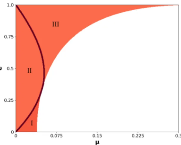
It is clear from the coefficientsJ_ithat Eqs. (25)-(28) do not have solutions ifq^(l)_jk(µ,e) =0 (j=1 or 2, k=1 or 2 andl=1 or 2,see Eqs. (15)-(18)). The forbidden parameter pairs (µ,e) as solid lines are depicted in Fig.1. We note thatq⁽¹⁾₁₂ andq⁽²⁾₁₂ associated to Eqs. (25) and (27) do not take zero value anywhere in the shaded region. However, the black solid line between domain I and II corresponds to those (µ,e) pairs where q⁽¹⁾₂₁ =0.Similarly,q⁽²⁾₂₁ =0 along the line between the regions II and III.

Fig. 1:Shaded region ofµ−eparameter plane describes where Hill’s equations might have real solutions. Along the black solid lines between domains I, II, and III. conditionq⁽ⁱ⁾₂₁=0 holds. That is Eqs. (27) and (28) have no solutions. No stable solution exists in white part.

Transformations Eqs. (23)-(24) can be substituted into Eq. (22), from which we get

y2=



 q⁽¹⁾₂₂ r|q⁽¹⁾₁₂|^3/2

− q⁽¹⁾₁₁ q

|q⁽¹⁾₁₂|



ξ1+ 1 r

q

|q⁽¹⁾₁₂|

ξ₁⁰ and y^∗₂=



 q⁽²⁾₂₂ r|q⁽²⁾₁₂|^3/2

− q⁽²⁾₁₁ q

|q⁽²⁾₁₂|



ξ2+ 1 r

q

|q⁽²⁾₁₂| ξ₂⁰.

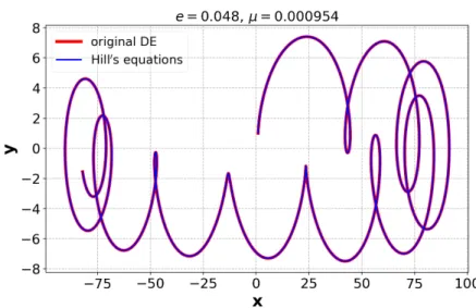
(29) Doing this Eq. (29) reduces the four Hills equations to two. Thus Eqs. (25) and (27) fully describe the problem¹. In other words, Eqs. (29) allows one to use safely the transformations (23) and (24) to solve Hill’s equations. Fig.2depicts the trajectory for e=0.048,µ=0.000954 (the case of Jupiter). The solution of Eqs. (1)-(2) and Eqs. (25)-(27) originating from the appropriate initial conditions perfectly overlap. This means, that the transformations Eqs. (23)-(24) lead to the same result, therefore, Hill’s equations can be applied to solve the equations of motion around theL₄andL₅points.

1 We note that any two equations can be selected but for practical reasons the pair ofξ1andξ2is the best choice.

Fig. 2:Numerical solutions around theL4andL5points. The initial conditions and the parameters arex0=1,y0=1,vx0=0,vy0=0, e=0.048,µ=0.000954 (the case of Jupiter), respectively.

3 Perturbative solution

In this section we give the perturbative solution of the differential equations. Hill’s equations (Eqs. (25)- (27)), as they are second order differential equations with periodic coefficients, can be solved by Floquet theorem [Hagel(1992)]. We seek the solution in the form of

ξ(v) =aw(v)cos(ψ(v) +b), (30) wherew(v) is the so-called Floquet function, which has the same period asξ(v). Constantsa andb are determined by the initial conditions. Since the derivation for both ξ₁ and ξ₂ are the same, we omit the indices in the rest part of the paper. Let us rewrite Eqs. (25)-(27) tow(v)andψ(v)

ξ⁰(v) =aw⁰(v)cos(ψ(v) +b)−aw(v)sin(ψ(v) +b)ψ⁰(v), (31) ξ⁰⁰(v) =aw⁰⁰(v)cos(ψ(v) +b)−2aw⁰(v)sin(ψ(v) +b)ψ⁰(v)−aw(v)cos(ψ(v) +b)ψ⁰²(v)

−aw(v)sin(ψ(v) +b)ψ⁰⁰(v). (32)

The differential equations above split into two parts with the coefficients of sin and cos

w⁰⁰(v)−w(v)ψ⁰²(v) +J(v)w(v) =0, (33) 2w⁰(v)ψ⁰(v) +w(v)ψ⁰⁰(v) =0. (34) From Eq. (34) we obtain

2w⁰(v)

w(v) =−ψ⁰⁰(v)

ψ⁰(v) ⇒ d

dvlog(w²(v)) = d dvlog

1 ψ⁰(v)

⇒ ψ⁰(v) = C

w²(v), (35) whereCis a constant. With this equation Eq. (33) becomes

w⁰⁰+J(v)w(v)− C²

w³(v)=0. (36)

Now we are looking for the solution ofw(v)in a third order Taylor series in the eccentricitye

w(v) =w⁽⁰⁾(v) +ew⁽¹⁾(v) +e²w⁽²⁾(v) +e³w⁽³⁾(v) +O(e⁴). (37) 3.1 Taylor series ofJ₁(v)andJ₂(v)

The periodic coefficients to be solved have complicated forms, therefore, the solution can be obtained by a third order Taylor expansion in the eccentricity. Let us first utilizeJ₁

J₁(v)=−

( c₁r+2−

3

2(1−c+3ecos(v))+c2 1

4(2c2+1−c)+ecos(v)−¹₄ke²cos(2v)+3 −¹₂esin(v)(1−kecos(v))

1

4(2c2+1−c)+ecos(v)−¹₄ke²cos(2v)

!2) , (38) by using the earlier introduced notations. Useful expressions will beλ≡√

1−9gandB≡(2c₂+1−λ)⁻¹. Third order Taylor expansion ofJ1is then

J1(v;e,µ) =α1+β1cos(v)e+ (γ₁+δ₁cos(2v))e²+ (ε₁cos(v) +η1cos(3v))e³+O(e⁴), where

α₁=−c₁−2+B(6−6λ+4c₂), β1=c1+18B+8B²(−3+3λ−2c2),

γ₁=B²

λ (6−12λ+4c₂)−6B λ −c₁

2 −4B³(10c₂−3+3λ), δ1=B²k

6−6λ+4c₂+6 k

−c₁

2 −4B³(10c₂−3+3λ), ε1=B⁴

λ

(20c₂−6+30λ+10c₂λk−3λk+3λ²k

B +6kλ

B² +64c²₂+32c₂+ (39) +208c₂λ−32c₂kλ−12kλ+24k−216gk+32c2k−288kc₂g−12kλ³−16c²₂kλ−

−72λ+72−648g )

+3c₁ 4 , η₁=B⁴

λ

(10c₂λk−3λk+3λ²k+24λ

B +6kλ

B² −32c₂kλ−12kλ+24k−216gk+

+32c₂k−288c₂gk−12kλ³−16c²₂kλ+80λc₂−24λ+24−216g )

+c1

4. The expression of the other periodic coefficientJ₂is

J

(v)=−

(

c

r+2−

4(2c₂+1+c)+ecos(v)−¹₄ke²cos(2v)

+3

4(2c₂+1+c)+ecos(v)−¹₄ke²cos(2v)

) .

J₂(v;e,µ) =α2+β2cos(v)e+ (γ₂+δ₂cos(2v))e²+ (ε₂cos(v) +η2cos(3v))e³+O(e⁴),

where

α2=−c₁−2+D(6+6λ+4c₂), β2=c₁+18D−8D²(3+3λ+2c₂),

γ2=−D²

λ (6+12λ+4c2) +6D λ −c1

2 +4D³(−10c₂+3+3λ), δ₂=D²k

6+6λ+4c₂+6 k

−c1

2 +4D³(−10c₂+3+3λ), (41) ε2=D⁴

λ

(−20c₂+6+30λ+10c₂λk−3λk−3λ²k

D +6kλ

D² −64c²₂−32c₂+

+208c₂λ−32c₂kλ−12kλ−24k+216gk−32c₂k+288kc₂g−12kλ³−16c²₂kλ−

−72λ−72+648g )

+3c₁ 4 , η2=D⁴

λ

(10c₂λk−3λk−3λ²k+24λ

D +6kλ

D² −32c2kλ−12kλ−24k+216gk−

−32c₂k+288c₂gk−12kλ³−16c²₂kλ+80λc₂−24λ−24+216g )

+c₁ 4. Let us write back the results of the Taylor expansions into Eq. (36), and use the fact that

1

(w⁽⁰⁾(v)+ew⁽¹⁾(v)+e²w⁽²⁾(v)+e³w⁽³⁾(v))³= 1

w⁽⁰⁾³(v)−3w⁽¹⁾(v)

w⁽⁰⁾⁴(v)e+6w⁽¹⁾²(v)−3w⁽⁰⁾(v)w⁽²⁾(v) w⁽⁰⁾⁵(v) e²+ +−3w⁽⁰⁾²(v)w⁽³⁾(v) +12w⁽⁰⁾(v)w⁽¹⁾(v)w⁽²⁾(v)−10w⁽¹⁾³(v)

w⁽⁰⁾⁶(v) e³+O(e⁴).

(42)

Then we can collect the terms fore⁰,e¹,e²ande³, thus 4 new differential equations can be obtained (also fori=1,2) for the terms ofw(v):

w⁽⁰⁾⁰⁰(v) +w⁽⁰⁾(v)α− C²

w⁽⁰⁾³(v)=0, (43)

w⁽¹⁾⁰⁰(v) +w⁽⁰⁾(v)βcos(v) +w⁽¹⁾(v)α+3C²w⁽¹⁾(v)

w⁽⁰⁾⁴(v) =0, (44)

w⁽²⁾⁰⁰(v) +w⁽⁰⁾(v)

γ+δcos(2v)

+w⁽¹⁾(v)βcos(v) +w⁽²⁾(v)α−6C²w⁽¹⁾²(v)

w⁽⁰⁾⁵ +3C²w⁽²⁾(v)

w⁽⁰⁾⁴(v) =0, (45) w⁽³⁾⁰⁰(v) +w⁽⁰⁾(v)

εcos(v) +ηcos(3v)

+w⁽¹⁾(v)

γ+δcos(2v)

+w⁽²⁾βcos(v) +w⁽³⁾(v)α+ +3C²w⁽³⁾(v)

w⁽⁰⁾⁴(v) −12C²w⁽¹⁾(v)w⁽²⁾(v)

w⁽⁰⁾⁵(v) +10C²w⁽¹⁾³(v) w⁽⁰⁾⁶(v) =0.

(46)

Again we note, that for all casesw^(j)(v) =w^(j)(v+2π),(j=0,1,2,3), as alsoξ(v) =ξ(v+2π). It can be easily seen, that the unique solution for Eq. (43) is:

w⁽⁰⁾(v) =C^1/2

α^1/4 ≡w_0,0. (47)

Differential equations (44)-(45)-(46) are second order linear differential equations, therefore the solution can be written up as the sum of the solution of the homogeneous equation (w⁽_h^j)(v)) and a particular solution of the inhomogeneous equation (w⁽_ih^j)(v)). Homogeneous part of Eq. (44) is

w⁽¹⁾

00

h (v) + α+3C² w⁴_0,0

!

w⁽¹⁾_h (v) =0, (48)

which is a harmonic oscillator with frequency

α+^3C2

w⁴_0,0

1/2

, thus the solution of the equation is

w⁽¹⁾_h (v) =K₁sin s

α+3C² w⁴_0,0v

!

+K₂cos s

α+3C² w⁴_0,0v

!

, (49)

where the constants K₁ andK₂ must be determined from the initial conditions. In order to fulfill the 2π periodicity ofw(v), the constants must beK1=K2≡0. For the inhomogeneous solution we use the following trial function

w⁽¹⁾_ih (v) =w1,1cos(v) +w1,0, (50) wherew1,1arew1,0constants. By calculating the derivatives from the coefficients we can simply obtain the values ofw_1,1andw_1,0, namely

w1,1=− w_0,0β α+3C²

w⁴_0,0−1

, w1,0=0. (51)

We use the same steps for the solution of Eq. (45). By using trigonometric identities it can be seen, that the differential equation has the following form

w⁽²⁾⁰⁰(v)+ α+3C² w⁴_0,0

!

w⁽²⁾(v)= −w_0,0γ−1

2w_1,1β+3C²w²_1,1 w⁵_0,0

!

− w_0,0δ+1

2w_1,1β−3C²w²_1,1 w⁵_0,0

!

cos(2v).

(52) Like in the previous case the solution of the homogeneous part is

w⁽²⁾_h (v) =K₁sin s

α+3C² w⁴_0,0v

!

+K₂cos s

α+3C² w⁴_0,0v

!

, (53)

where againK₁andK₂must disappear for the 2πperiodicity,K₁=K₂≡0. The trial function of the particular solution of the inhomogeneous equation is:

w⁽²⁾_ih (v) =w2,2cos(2v) +w2,0. (54)

Again by calculating the appropriate derivatives the equality of the coefficients imply:

w2,2=

3C²w²_1,1

w⁵_0,0 −w0,0δ−1 2w1,1β α+3C²

w⁴_0,0−4

, w2,0=

3C²w²_1,1

w⁵_0,0 −w0,0γ−1 2w1,1β α+3C²

w⁴_0,0

. (55)

Only the solution of Eq. (46) is left

w⁽³⁾⁰⁰(v) +w⁽³⁾(v) α+3C² w⁴_0,0

!

=− w0,0ε+w1,1γ+1

2w1,1δ+w2,0β+1

2w2,2β−12C²w1,1w2,0

w⁵_0,0 −

−6C²w_1,1w_2,2

w⁵_0,0 +15C²w³_1,1 2w⁶_0,0

!

cos(v)− w0,0η+1

2w1,1δ+1

2w2,2β−6C²w_1,1w_2,2

w⁵_0,0 +5C²w³_1,1 2w⁶_0,0

!

cos(3v).

(56) The homogeneous solution reads

w⁽³⁾_h (v) =K₁sin s

α+3C² w⁴_0,0v

!

+K₂cos s

α+3C² w⁴_0,0v

!

, (57)

where again the constants areK₁=K₂≡0 due to the periodicity ofw(v). The trial function for the particular solution of the inhomogeneous equation

w⁽³⁾_ih(v) =w_3,1cos(v) +w_3,3cos(3v), (58) where the forms forw3,1andw3,3coefficients are

w_3,1=−

w_0,0ε+w_1,1γ+1

2w_1,1δ+w_2,0β+1

2w_2,2β−12C²w_1,1w_2,0

w⁵_0,0 −6C²w_1,1w_2,2

w⁵_0,0 +15C²w³_1,1 2w⁶_0,0 α+3C²

w⁴_0,0−1

,

w_3,3=−

w_0,0η+1

2w_1,1δ+1

2w_2,2β−6C²w_1,1w_2,2

w⁵_0,0 +5C²w³_1,1 2w⁶_0,0 α+3C²

w⁴_0,0−9

.

(59)

Then by using the fact thatψ⁰(v) =Cw⁻²(v), Eq. (33),ψ(v)can be calculated if we again expandψ⁰(v)into Taylor series ineup to third order

1

Cψ(v) = v

w²_0,0−2w_1,1sin(v) w³_0,0 e+ 1

w⁴_0,0 (

3w²_1,1

sin(2v) 4 +v

2

−w_0,0w_2,0v−sin(2v)w_0,0w_2,2 2

) e²−

− 1 w⁵_0,0

(2 3w³_1,1

9

4sin(v)+sin(3v) 4

+sin(v)w²_0,0w_3,1+sin(3v)w²_0,0w_3,3

3 −2 sin(v)w_0,0w_1,1w_2,0−

−2w_0,0w_1,1w_2,2 sin(v)

2 +sin(3v) 6

+2

3w_1,1 w²_1,1

4 −w0,0w2,2

2

!

sin(3v)+

+2w1,1

3

4w²_1,1−1

2w0,0w2,2−w0,0w2,0

sin(v)

)

e³+O(e⁴).

(60) Now we have expressions forw(v)andψ(v), thusξ(v) =aw(v)cos ψ(v) +b

can be calculated. One can easily see, that allwi,jcoefficients and the expression ofψ(v)have a common multiplicative factor√

Cand C respectively, therefore this factor can be chosen to beC=1. The effects ofC will be considered with the initial conditions. It is left to determine constantsaandb, which are controlled by the initial conditions ξ(0)≡ξ0andξ⁰(0)≡ξ₀⁰. As the differential equations are second order linear differential equations with periodic coefficients, the initial conditions can be arbitrary, therefore we use the simple conditions ofx₀=1, y₀=1,v_x0=0,v_y0=0, from whichξ1,0,ξ_1,0⁰ ,ξ2,0andξ_2,0⁰ can be easily achieved. By using the valuesξ0

andξ₀⁰

ξ0=aw(0)cos ψ(0) +b

, ξ₀⁰=aw⁰(0)cos ψ(0) +b

− 1

w(0)sin ψ(0) +b

, therefore

a= s

w⁰(0)ξ₀−ξ₀⁰w(0)2

+ ξ0

w(0) 2

, b=arccos ξ0

aw(0)

−ψ(0).

(61)

At the end the only task is to use the transformations detailed in Eqs. (23)-(24), calculatey2 andy^∗₂with Eq. (29), then turn back to thex,ycoordinates asx=y1+y^∗₁andy=y2+y^∗₂.

4 Illustrations and discussion

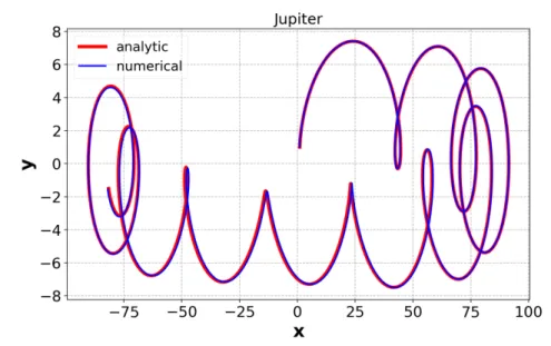
The prominent example of co-orbital dynamics is the Sun-Jupiter-Trojan configuration in our own Solar System. We apply the perturbative solution described in Sec.3.1to this structure first. Fig.3 depicts the trajectory around the Sun-Jupiter triangular Lagrangian point. The integration time is 20 periods of Jupiter (ca. 240 years). The analytic and numerical solutions match perfectly, although after some time (∼38−40 periods) they start to deviate.

Recently, [Lillo-Box et al(2018)Lillo-Box, Leleu, Parviainen, Figueira, Mallonn, Correia, Santos, Robutel, Lendl, Boffin, Faria, Barrado, and Neal]

studied the physical parameters and dynamical properties of possible exo-Trojans in systems with close-in (orbital period<5 days) planets. We selected two of them, HAT-P-20b (e=0.015,µ=0.0091) and WASP- 36b (e=0.0, µ=0.0021), to demonstrate analytic solution in these regimes². The orbits are plotted in

2 The orbital periods are HAT-P-20b : 2.87 days, WASP-36b : 1.53 days.

Fig. 3:Analytic and numerical solution in Sun-Jupiter system. Initial conditions are the same as in Fig2.

Fig.4a and b, respectively. The panels show the paths for T=20 periods again. Due to the zero eccentricity of the planet, the analytic solution for WASP-36b remains very close to the numerical outcome for much longer times (not shown here).

Fig. 4:Perturbative solution for particular exoplanetary systems. Initial conditions are the same as in Fig2. For parameters see the main text.

Considering the Earth-Moon system withe=0.054 and µ=0.012 it falls close to the limit of third order solution. The analytic solution diverges after 5-6 revolutions (∼130−150 days) of the Moon. We have seen that for Sun-Jupiter system the analytic curve traces the numerical method reasonable well while the eccentricity falls into the same range. In addition, we have found that the rather large mass parameter - compared to planetary systems - does not affect the precision of the analytic solution provided the eccentric- ity is small enough, practically zero. This is, however, not the case for Moon. Consequently, systems with

moderate non-zero eccentricity and mass parameter in the same magnitude requires further improvement to the analytic solution, e.g. higher order expansion in mass.

In this work we fully describe the motion around triangular Lagrangian points with Hill’s equations.

As a perturbative solution, a third order expansion of Floquet function w(v)in eccentricity is presented.

This method is capable to follow analytically the orbit of a massless particle around the equilibrium points L₄and L₅in ERTBP. Precise trajectory forecast for moderate eccentricity (e≤0.05) and mass parameter (µ≤0.005) is achievable for tens of secondary’s orbital period. Furthermore, we note that Eq.61can be used to identify periodic orbits around L₄and L₅points. This calculation is postponed elsewhere.

Acknowledgements This work was supported by the NKFIH Hungarian Grants K119993, FK134203. The support of Bolyai Research Fellowship and ´UNKP-19-2 (BB) and ´UNKP-19-4 (TK) New National Excellence Program of Ministry for Innovation and Technology is also acknowledged.

References

Danby(1964). Danby JMA (1964) Stability of the triangular points in the elliptic restricted problem of three bodies. The Astronomical Journal 69:165, DOI 10.1086/109254

Erdi(1974). Erdi B (1974) Reduction of the two-dimensional elliptic restricted problem of three bodies to Hill’s Equation . The Astro- nomical Journal 79:653, DOI 10.1086/111592

Erdi(1977). Erdi B (1977) An Asymptotic Solution for the Trojan Case of the Plane Elliptic Restricted Problem of Three Bodies.

Celestial Mechanics 15(3):367–383, DOI 10.1007/BF01228428

Erdi(1978). Erdi B (1978) The Three-Dimensional Motion of Trojan Asteroids. Celestial Mechanics 18(2):141–161, DOI 10.1007/

BF01228712

Hagel(1992). Hagel J (1992) A New Analytic Approach to the Sitnikov Problem. Celestial Mechanics and Dynamical Astronomy 53(3):267–292, DOI 10.1007/BF00052614

Lichtenberg and Lieberman(1983). Lichtenberg AJ, Lieberman MA (1983) Regular and stochastic motion. Springer-Verlag

Lillo-Box et al(2018)Lillo-Box, Leleu, Parviainen, Figueira, Mallonn, Correia, Santos, Robutel, Lendl, Boffin, Faria, Barrado, and Neal.

Lillo-Box J, Leleu A, Parviainen H, Figueira P, Mallonn M, Correia ACM, Santos NC, Robutel P, Lendl M, Boffin HMJ, Faria JP, Barrado D, Neal J (2018) The TROY project. II. Multi-technique constraints on exotrojans in nine planetary systems. Astronomy and Astrophysics 618:A42, DOI 10.1051/0004-6361/201833312,1807.00773

Matas(1982). Matas VR (1982) A Note on a Separation of the Linearized Equations of Motion in the Elliptic Restricted Problem.

Celestial Mechanics 27(1):23–25, DOI 10.1007/BF01228947

Meire(1980). Meire R (1980) A Contribution to the Stability of the Triangular Points in the Elliptic Restricted Three-body Problem.

Bulletin of the Astronomical Institutes of Czechoslovakia 31:312

Meire(1981). Meire R (1981) The Stability of the Triangular Points in the Elliptic Restricted Problem. Celestial Mechanics 23(1):89–

95, DOI 10.1007/BF01228547

Meire(1982). Meire R (1982) On the Stability of the Triangular Points in the Elliptic Restricted Problem. Astronomy and Astrophysics 110:152

Morais(2001). Morais MHM (2001) Hamiltonian formulation of the secular theory for Trojan-type motion. Astronomy and Astro- physics 369:677–689, DOI 10.1051/0004-6361:20010141

P´aez et al(2016)P´aez, Locatelli, and Efthymiopoulos. P´aez RI, Locatelli U, Efthymiopoulos C (2016) The Trojan Problem from a Hamiltonian Perturbative Perspective. Astrophysics and Space Science Proceedings 44:193, DOI 10.1007/978-3-319-23986-6 14 Robutel et al(2016)Robutel, Niederman, and Pousse. Robutel P, Niederman L, Pousse A (2016) Rigorous treatment of the averaging

process for co-orbital motions in the planetary problem. Comp Appl Math 35:675–699, DOI 10.1007/s40314-015-0288-2 Szebehely(1967). Szebehely V (1967) Theory of orbits. The restricted problem of three bodies. Academic Press

Tschauner(1971). Tschauner J (1971) Die Bewegung in der N¨ahe der Dreieckspunkte des elliptischen eingeschr¨ankten Dreik¨orperproblems. Celestial Mechanics 3(2):189–196, DOI 10.1007/BF01228032