AIMS’ Journals
VolumeX, Number0X, XX200X pp.X–XX
STABLE PERIODIC SOLUTIONS FOR NAZARENKO’S
1
EQUATION
2
Szandra Beretka
Bolyai Institute, University of Szeged 1 Aradi v´ertan´uk tere, Szeged, Hungary
Gabriella Vas∗
MTA-SZTE Analysis and Stochastics Research Group, Bolyai Institute, University of Szeged 1 Aradi v´ertan´uk tere, Szeged, Hungary
(Communicated by the associate editor name)
Abstract. In 1976 Nazarenko proposed studying the delay differential equa- tion
˙
y(t) =−py(t) + qy(t)
r+yn(t−τ), t >0,
under the assumptions thatp, q, r, τ ∈(0,∞),n∈N={1,2, . . .}andq/p > r.
We show that if τ or n is large enough, then the positive periodic solution oscillating slowly aboutK = (q/p−r)1/nis unique, and the corresponding periodic orbit is asymptotically stable. We also determine the asymptotic shape of the periodic solution asn→ ∞.
1. Introduction. We consider the scalar delay differential equation
3
˙
y(t) =−py(t) + qy(t)
r+yn(t−τ), t >0, (1) under the assumption that
4
p, q, r, τ∈(0,∞), n∈N={1,2, . . .} and q
p > r. (2) This equation was proposed by Nazarenko in 1976 to study the control of a
5
single population of cells [9]. The quantityy(t) is the size of the population at time
6
t. The rate of change y0(t) can be given as the difference of the production rate
7
qy(t)/(r+yn(t−τ)) and the destruction rate py(t). We see that the destruction
8
rate at time t depends only on the present state y(t) of the system, while the
9
production rate also depends on the past ofy. This is a typical concept in population
10
dynamics; delay appears due to the fact that organisms need time to mature before
11
reproduction.
12
For further population model equations with delay, see e.g., [14]. One of the most
13
widely studied examples is the Mackey-Glass equation:
14
˙
y(t) =−py(t) + qy(t−1)
r+yn(t−τ), t >0. (3)
2010Mathematics Subject Classification. Primary: 34K13, 92D25; Secondary: 34K27.
Key words and phrases. Delay differential equation, Periodic solution, Uniqueness, Stability.
∗Corresponding author: G. Vas.
1
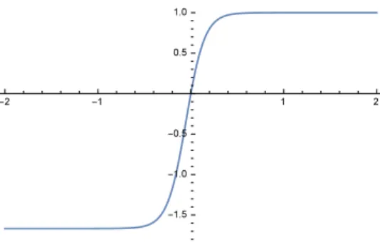
Figure 1. The plot of f forp= 1,q= 4, r= 1.5 andn= 10
In this model the production rate is very similar to the one considered by Nazarenko.
1
The usual phase space for (1) is the Banach spaceC =C([−τ,0],R) with the
2
supremum norm. A solution of (1) is either a continuously differentiable function
3
y:R→Rthat satisfies (1) for allt∈R, or a continuous function y: [−τ,∞)→R
4
that is continuously differentiable for t > 0 and satisfies (1) for all t > 0. If for
5
some solution y and t ∈ R, the interval [t−τ, t] is in the domain of y, then the
6
segmentyt∈C is defined byyt(s) =y(t+s) for−τ ≤s≤0. To eachφ∈C there
7
corresponds a solution yφ: [−τ,∞) → R with yφ0 = φ. Under condition (2), the
8
functionsR3t7→0∈RandR3t7→K= (q/p−r)1/n∈Rare the only constant
9
solutions, i.e., there exists a unique positive equilibrium besides the trivial one.
10
Several authors have already examined equation (1), see e.g., the works [5,6,17,
11
19]. In this paper we focus on those positive periodic solutions of (1) that oscillate
12
slowly about K. A solution y is called slowly oscillatory about K if all zeros of
13
y−K are spaced at distances greater than the delayτ. It is widespread to use the
14
abbreviation SOP for such periodic solutions.
15
If we restrict our examinations only to positive solutions, then we can apply the
16
transformationx= logy−logK. Thereby we obtain the equation
17
x0(t) =−f(x(t−τ)), (4)
where the feedback functionf ∈C1(R,R) is defined as
18
f(x) =p− q r+q
p−r enx
for allx∈R, (5)
see Fig. 1. Note that f(0) = 0. Condition (2) implies thatf is strictly increasing,
19
hence we are in the so called “negative feedback” case. Solutions and segments of
20
solutions of (4) are defined analogously as for equation (1). Note that the positive
21
equilibrium of (1) given byK is transformed into the trivial equilibrium of (4). In
22
accordance, an SOP solution of (4) is a periodic solution that have zeros spaced at
23
distances greater than τ. We know from Theorem 7.1 of Mallet-Paret and Sell in
24
[8] that ifT0< T1< T2 are three consecutive zeros of an SOP solution of (4), then
25
T2−T0 is its minimal period.
26
Nussbaum verified the global existence of SOP solutions for equations of the form
27
(4) and for a wide class of feedback functions containing (5), see [11] and also [10].
28
His proof applies the Browder ejective fixed point principle. By [10, 11], equation
29
(4) has at least one SOP solution for
1
τ > τ0= π
2f0(0) = qπ 2np(q−pr).
Nussbaum also established results on the uniqueness of the SOP solution (up
2
to translation of time) in [13]. However, paper [13] demandsf to be odd, thus it
3
cannot be applied for (5). Paper [2] of Cao, a second result on uniqueness, requires
4
h(x) = xf0(x)/f(x) < 1 to be monotone decreasing in x ∈ (0, b) and monotone
5
increasing in x∈ (−a,0) with some a > 0 and b >0. One can easily check that
6
this concavity condition does not necessarily hold in our case either. We need to
7
choose a different approach to guarantee the uniqueness of the SOP solution. The
8
monotonicity off is not sufficient: Cao proved the existence of a monotone f in [1]
9
such that equation (4) has at least two distinct SOP solutions.
10
The stability of the SOP solutions is another central question. A well-known
11
result is due to Kaplan and Yorke [3]: under certain restrictions on f, if the SOP
12
solution is unique, then it is orbitally asymptotically stable. The region of attraction
13
consists of the segments of all eventually slowly oscillatory solutions.
14
For a more detailed summary on SOP solutions of equation (4), we refer to the
15
work [4] of Kennedy and Stumpf.
16
Song, Wei and Han studied the equation in the form (1), and they showed that
17
a series of Hopf bifurcations takes place at the positive equilibrium as τ passes
18
through the critical values
19
τk = 1 f0(0)
π
2 + 2kπ
= q
np(q−pr) π
2 + 2kπ
, k≥0,
see [17]. They gave explicit formulae to determine the stability, direction and the
20
period of the bifurcating periodic solutions. Then they verified the global existence
21
of the bifurcating periodic solutions by applying the global Hopf bifurcation theory
22
in [20]. They showed that equation (1) has at leastk periodic solutions ifτ > τk,
23
k ≥1. Song, Wei and Han could not decide whether equation (1) has a periodic
24
solution ifτ ∈(τ0, τ1). As we have mentioned above, Nussbaum solved this problem
25
in [11].
26
Our work is motivated by the fact that Song and his coauthors could not deter-
27
mine the stability of the periodic orbits forτfar away from the local Hopf bifurcation
28
values. Uniqueness of the SOP solution has not been studied either.
29
The following theorems are the main results of this paper.
30
Theorem 1.1. Set p, q, randn as in (2).
(i) If τ > 0 is large enough, then equation (1) has a unique positive periodic so- lution y¯: R→ R oscillating slowly about K. The corresponding periodic orbit is asymptotically stable, and it attracts the set
n
φ:yφ(t)>0fort≥ −τ, yφt −K has at most one sign change for large to . (ii) Ifω¯ denotes the minimal period ofy, and¯
31
ω=
2 + q−pr
pr + pr
q−pr
τ, (6)
thenlimτ→∞ω/ω¯ = 1.
32
Uniqueness of the periodic solution is always meant up to time translation.
33
If we fix p, q, r and τ, we can determine the asymptotic shape of the periodic
34
solution asn→ ∞.
35
Theorem 1.2. Set p, q, randτ such that (2) and τmin{p, q/r−p}>8 hold.
1
(i) Theorem1.1.(i) is true for all sufficiently largen.
2
(ii) Definev:R→Ras theω-periodic extension of the piecewise linear function
3
[0, ω]3t7→
−pt, 0≤t < τ,
q r−p
t−qrτ, τ ≤t <
2 +q−prpr τ,
−pt+
q
r+p+q−prp2r
τ,
2 + q−prpr
τ ≤t < ω
∈R,
where ω is given by (6). Letη1>0 andη2 >0 be arbitrary. If nis large enough, then there exists T ∈Rfor theω-periodic SOP solution¯ y, such that¯ |¯ω−ω|< η1, and
logy(t¯ +T) K −v(t)
< η2 for allt∈[0,ω].¯
The proofs of these theorems are similar, and they are organized as follows.
4
Throughout the paper we examine equation (1) in the form (4)-(5). First we cal-
5
culate an SOP solution v for the ”limit equation” v0(t) = −g(v(t−τ)), where
6
g:R→Ris a piecewise constant function chosen so that (5) is close tog outside
7
a neighborhood of 0. Then we consider (5) as a perturbation ofg and follow the
8
technique used by Walther in [18] (for a slightly different class of equations) to ob-
9
tain information about the solutions of equation (4). We show the existence of a
10
convex closed subsetA(β)⊆Csuch that all solutions of (4) with initial segments in
11
A(β) return toA(β). Thereby a return map P:A(β)→ A(β) can be introduced.
12
Next we explicitly evaluate a Lipschitz constant L(P) for P. If τ or n is large
13
enough, thenL(P)<1, i.e.,P is a contraction. The unique fixed point of P is the
14
initial segment of an SOP solution. Besides this, we need the results of paper [12]
15
of Nussbaum to show that all SOP solutions have segments inA(β), and hence the
16
SOP solution is unique. The rest of the theorems will follow easily. In particular,
17
stability comes from the work [3] of Kaplan and Yorke.
18
We give full proofs only when
19
q
pr and pr
q−pr (7)
are not integers. In this case we determine the sizes ofτandnexactly. We indicate
20
the necessary modifications when eitherq/(pr) orpr/(q−pr) is an integer.
21
The particular form of f is actually not important. It is possible to show that equation (4) admits an SOP solution if the feedback function f is Lipschitz- continuous, there are constantsA >0,B >0 and smallβ >0 such that
|f(x) +A|is small forx <−β and |f(x)−B|is small forx > β, furthermore, the Lipschitz constant for f restricted to the interval (−∞,−β]∪
22
[β,∞) is also sufficiently small. The method of Walther in [18] works for all such
23
nonlinearities. If, in addition,f(0) = 0,f is continuously differentiable andf0(x)>
24
0 for all real x, then one can prove uniqueness and stability using papers [12] of
25
Nussbaum and [3] of Kaplan and Yorke.
26
Let us also mention that the Schwarzian derivative of (5) equals −n2/2 at all x ∈ R. Hence Proposition 2 of Liz and R¨ost in [7] gives bounds for the global attractor: Ifτ f0(0)>3/2, then
α≤lim inf
t→∞ x(t)≤lim sup
t→∞
x(t)≤β
for all solutions xof (4), where {α, β} is the unique 2-cycle ofx7→ −τ f(x) (that is,β =−τ f(α) andα=−τ f(β)). In consequence,
Keα≤lim inf
t→∞ y(t)≤lim sup
t→∞
y(t)≤Keβ
for all positive solutionsy of (1). If τ f0(0)≤3/2, then Proposition 2 of [7] states
1
that all solutions of (4) converge to 0 (and hence all positive solutions of (1) converge
2
to K) as t → ∞. This result improves the well-known fact that the trivial equi-
3
librium of (4) (and hence the positive equilibrium of (1)) is locally asymptotically
4
stable wheneverτ f0(0)< π/2.
5
2. The limit equation. Consider equation (4) with feedback function (5). Let
6
A=q/r−p >0 andB=p >0.
7
Note that ifp, q, rare fixed according to (2), thenf(x) converges top−q/r=−A
8
as nx→ −∞ and f(x) tends to p= B as nx → ∞. Therefore we examine the
9
”limit equation”
10
v0(t) =−gA,B(v(t−τ)), (8)
wheregA,B:R→Ris defined as
11
gA,B(v) =
−A, v <0, 0, v= 0, B, v >0.
Given anyφ∈C, a solutionvφ: [−τ,∞)→Rof (8) is an absolutely continuous
12
function such thatvφ|[−τ,0]=φand the integral equation
13
vφ(t) =vφ(0)− Z t
0
gA,B vφ(s−τ)
ds (9)
is satisfied for t >0. Similarly, an absolutely continuous function v: R→ R is a
14
solution of (8), if the integral equation is satisfied for allt∈R.
15
In this section we evaluate an SOP solution for (8).
16
Proposition 1. Equation (8) admits a periodic solution v : R → R defined as follows:
v(t) =
−Bt, t∈[0, τ],
At−(A+B)τ, t∈[τ, σ+τ],
−Bt+
A+ 2B+BA2
τ, t∈[σ+τ, ω],
whereσ= (1 +B/A)τ is the first positive zero, andω= (2 +A/B+B/A)τ is the
17
second positive zero and the minimal period ofv.
18
Proof. Consider anyφ∈C withφ(t)>0 for allt∈[−τ,0) andφ(0) = 0. Consider
19
the corresponding solutionv=vφ of (8). We havev0(t) =−B fort∈[0, τ), hence
20
v(t) = −Bt for t ∈ [0, τ]. Necessarily, v is negative on an interval (0, T) where
21
T > τ. Thenv0(t) =Afort∈(τ, T+τ) and
22
v(t) =At−(A+B)τ fort∈[τ, T+τ]. (10) This function has zero at σ = (1 +B/A)τ.So formula (10) is valid with T = σ.
23
The solutionv is positive on (σ, σ+τ] and v(σ+τ) =Aτ.
24
If ω > σ+τ is chosen such that v is positive on (σ, ω), then v0(t) = −B for
25
t∈(σ+τ, ω+τ). We deduce that
26
v(t) =−Bt+
A+ 2B+B2 A
τ, t∈[σ+τ, ω+τ]. (11)
-A -A+
B- B
-
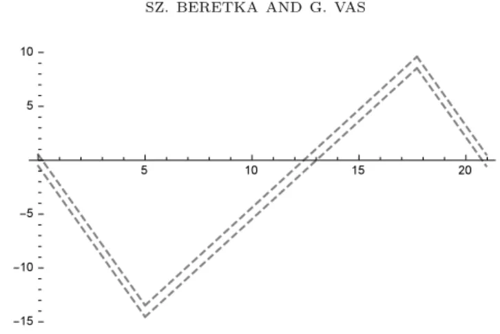
Figure 2. An element ofN(A, B, β, ε) From this formula we see thatω can be defined as
ω=
2 + A B +B
A
τ.
Note thatvω(t)>0 for allt∈[−τ,0) andvω(0) = 0. Hence, if we setφ=vω and
1
extendv|[−τ,ω]toRω-periodically, then we get a periodic solution of (8) onR.
2
3. Preliminary estimates. ForA >0,B >0,β >0, 0< ε <min{A, B}/2, let N(A, B, β, ε) denote the set of all continuous functionsf :R→Rwith
−A≤f(x)≤ −A+ε forx <−β,
−A≤f(x)≤B for −β≤x≤β, and
B−ε≤f(x)≤B forx > β,
see Fig. 2. Function (5) is an element of N(A, B, β, ε) if A = q/r−p, B = p, 0< ε <min{A, B}/2 and
β≥max
f−1(B−ε),−f−1(−A+ε) .
This is true because f(0) = 0, limx→−∞f(x) = −A, limx→∞f(x) = B and f is
3
strictly increasing.
4
Let
A(β) ={φ∈C:φ(t)≥β for −τ≤t≤0, φ(0) =β}.
In this section we study the solution x=xφ of (4) when f ∈ N(A, B, β, ε) and φ∈ A(β). Our main goal is to show that ifφ∈ A(β), then there existq >0 and
˜
q >0 such that
xq ∈ − A(β) ={φ∈C:φ(t)≤ −β for −τ≤t≤0, φ(0) =−β}, andxq+˜q∈ A(β).
5
Define the integerN by (N −1)τ < σ≤N τ, where σis the first positive zero
6
of the periodic functionvgiven by Proposition 1. Asσ= (1 +B/A)τ, we get that
7
N =d1 +B/Ae. The next proposition estimates|x(t)−v(t)|fort∈[0, N τ].
8
Proposition 2. Let A >0, B >0,β >0, 0< ε <min{A, B}/2,δ= 2β/(B−ε),
1
N =d1 +B/Ae,f ∈ N(A, B, β, ε) andφ∈ A(β). Assume that
2
c1=τ−δ >0 (C.1)
and
0< c2=
(B−2ε)τ−(2A+B)δ−2β if N = 2,
(A+B)(τ−δ)−(A+ε)(N−1)τ−2β if N >2. (C.2) Then
3
|x(t)−v(t)| ≤β+ετ for t∈[0, τ] (12) and
4
|x(t)−v(t)| ≤β+kετ+ (A+B)δ for2≤k≤N andt∈[(k−1)τ, kτ]. (13) Proof. Estimate (12). We know that v(0) = 0 and v(t)> 0 for t ∈ [−τ,0). For
5
t∈[0, τ],
6
|x(t)−v(t)|=
β− Z t
0
f(x(s−τ))ds+ Z t
0
Bds
≤β+ Z t
0
|B−f(x(s−τ))|ds
≤β+εt≤β+ετ.
(14)
So (12) holds.
7
It is also clear from the choice ofφthat x0(t)<0 for t∈(0, τ).
8
Proof of (13) for k = 2. Condition (C.1) guarantees that δ < τ, and therefore v(δ) =−Bδby Proposition 1. Then, by (14) and by the definition ofδ,
x(δ)≤v(δ) +β+εδ=−Bδ+β+εδ=−β.
By the monotonicity ofxon [0, τ], we obtain that
9
x(t)<−β fort∈(δ, τ]. (15)
For t∈ [0, δ], −A ≤f(x(t))≤B and thus|f(x(t)) +A| ≤ A+B. For t ∈[δ, τ],
|f(x(t)) +A| ≤εbecausex(t)≤ −β. These imply that Z τ
0
|f(x(s)) +A|ds= Z δ
0
|f(x(s)) +A|ds+ Z τ
δ
|f(x(s)) +A|ds
≤(A+B)δ+ε(τ−δ)≤(A+B)δ+ετ.
This observation together with (12) gives that fort∈[τ,2τ],
|x(t)−v(t)| ≤ |x(τ)−v(τ)|+ Z t
τ
|f(x(s−τ)) +A|ds
≤β+ετ+ (A+B)δ+ετ=β+ 2ετ+ (A+B)δ.
We have verified (13) fork= 2.
10
Proof of (13) for all 2< k≤N in case N >2 by induction on k. Assume that
11
(13) holds for a givenk∈ {2,3, ..., N−1}. We show that it holds fork+ 1. Recall
12
that
13
v(t) =At−(A+b)τ ≤A(N−1)τ−(A+B)τ <0 fort∈[τ,(N−1)τ]. (16) Using this, (C.2) and (13) for thisk, we obtain that fort∈[(k−1)τ, kτ],
x(t)≤v(t)+β+kετ+(A+B)δ≤A(N−1)τ−(A+B)τ+β+(N−1)ετ+(A+B)δ <−β.
Then, fort∈[kτ,(k+ 1)τ],
|x(t)−v(t)| ≤ |x(kτ)−v(kτ)|+ Z t
kτ
|f(x(s−τ)) +A|ds≤ |x(kτ)−v(kτ)|+ετ
≤β+ (k+ 1)ετ+ (A+B)δ.
Summing up, (13) is true for all 2≤k≤N.
1
The next proposition shows, among others, that to each φ∈ A(β) there corre-
2
spondsq∈(0, N τ) withxq ∈ −A(β).
3
Proposition 3. In addition to the assumptions of the previous proposition, suppose
4
that
5
c3= (A−ε)N τ−(A+B)(τ+δ)>0. (C.3) Then
6
x(t)<−β forδ < t≤max{τ+δ,(N−1)τ}, (17)
7
x(N τ)>−β, (18)
8
x0(t)<0fort∈(0, τ), (19)
9
x0(t)>0 fort∈(τ+δ, N τ), (20) and for the unique solutionq=q(φ) of the equationx(t) =−β in (τ+δ, N τ),
xq∈ −A(β).
If ψ∈ A(β)with xψδ+τ =xφδ+τ, thenq(φ) =q(ψ). Furthermore, ifτ B/A > δ, then
10
|q(φ)−σ| ≤ 1
A−ε(2β+N ετ+ (A+B)δ), (21) whereσ is the smallest positive zero ofv.
11
Proof. Inequality (17). We mentioned in the proof of Proposition2thatx(t)<−β fort∈(δ, τ], see (15). In case N = 2 we have max{τ+δ,(N−1)τ}=τ+δ. The formula
v(t) =At−(A+B)τ≤Aδ−Bτ, t∈[τ, τ+δ], estimate (13) withk= 2 and the first line of (C.2) together yield that
x(t)< v(t) +β+ 2ετ+ (A+B)δ≤Aδ−Bτ+β+ 2ετ+ (A+B)δ <−β for all t∈[τ, τ+δ]. IfN >2, then max{τ+δ,(N −1)τ}= (N−1)τ. A similar
12
argument (combining the second line of (C.2), estimate (13) with 2≤k ≤N−1
13
and also (16)) yields thatx(t)<−β fort∈[τ,(N−1)τ].
14
Inequality (18). We obtain (18) if we apply (13) for t=N τ, v(N τ) =AN τ−
15
(A+B)τ and (C.3):
16
x(N τ)> v(N τ)−(β+N ετ+ (A+B)δ) =c3−β >−β. (22) Estimates (19) and (20). It is clear from the choice of φ that x0(t) < 0 for
17
t∈(0, τ). By (17),x(t−τ)<−β fort∈(δ+τ, N τ], hence it is also clear that
18
x0(t) =−f(x(t−τ))≥A−ε >0 for t∈(δ+τ, N τ]. (23) Statements regarding q. Existence and uniqueness of the solution q = q(φ) ∈
19
(τ+δ, N τ) of xφ(t) = −β are now obvious from (17), (18) and (20). We see that
20
xφq ∈ −A(β).
21
It is also easy to see that if ψ ∈ A(β) with xψδ+τ = xφδ+τ, then q(φ) = q(ψ).
22
Indeed, this assertion comes from the facts thatxφ(t) =xψ(t) on [τ+δ,∞),q(φ)>
23
τ+δ andq(ψ)> τ+δ.
24
If in additionτ B/A > δ, then σ=τ+τ B/A > τ+δ. Hence we can apply (23) for alltbetweenσ∈(δ+τ, N τ] andq∈(δ+τ, N τ]:
(A−ε)|σ−q| ≤
Z σ q
f(x(t−τ))dt
=|x(σ)−x(q)|
≤|x(σ)−v(σ)|+|x(q)| ≤ |x(σ)−v(σ)|+β.
We obtain (21) from this by using (13) fort=σ∈[(N−1)τ, N τ].
1 2
We need analogous results for solutions with initial segments in −A(β). The
3
proofs of the subsequent two propositions can be easily brought back to the proofs
4
of Propositions2 and3.
5
Proposition 4. Let A >0,B >0,β >0,0< ε <min{A, B}/2, ˜δ= 2β/(A−ε),
6
N˜ =d1 +A/Be,f ∈ N(A, B, β, ε)andφ∈ −A(β). Assume that
7
c4=τ−δ >˜ 0, (C.4)
and
0< c5=
(A−2ε)τ−(A+ 2B)˜δ−2β if N˜ = 2,
(A+B)(τ−δ)˜ −(B+ε)( ˜N−1)τ−2β if N >˜ 2. (C.5) Then
8
|x(t)−v(t+σ)| ≤β+ετ for t∈[0, τ] (24) and
9
|x(t)−v(t+σ)| ≤β+kετ+ (A+B)˜δ for2≤k≤N˜ andt∈[(k−1)τ, kτ]. (25) Proposition 5. In addition to the assumptions of the previous proposition, suppose
10
that
11
c6= (B−ε) ˜N τ−(A+B)(τ+ ˜δ)>0. (C.6) Then
12
x(t)> β for δ < t˜ ≤max{τ+ ˜δ,( ˜N−1)τ}, (26)
13
x( ˜N τ)< β, (27)
14
x0(t)>0fort∈(0, τ), (28)
15
x0(t)<0 for t∈(τ+ ˜δ,N τ˜ ), (29) and for the unique solutionq˜= ˜q(φ) of the equationx(t) =β in(τ+ ˜δ,N τ˜ ),
xq˜∈ A(β).
If ψ∈ −A(β)with
xψ˜
δ+τ=xφ˜
δ+τ, thenq(φ) = ˜˜ q(ψ). Furthermore, ifτ A/B >˜δ, then
16
|q(φ)˜ −(ω−σ)| ≤ 1 B−ε
2β+ ˜N ετ+ (A+B)˜δ
. (30)
Proof of Proposition4and Proposition 5. Consider φ ∈ −A(β) and the solution x=xφ: [−τ,∞)→R. For ˜x: =−x, we have ˜x0∈ A(β) and
˜
x0(t) =−h(˜x(t−τ)) fort >0,
whereh:R3x7→ −f(−x)∈R. Observe thathis an element of the function class
17
N(B, A, β, ε).
18
In addition, define theω-periodic function ˜v:R→Ron [0, ω] as follows:
˜
v(t) =−v(t+σ) =
−At, t∈[0, τ],
Bt−(A+B)τ, t∈
τ, 2 +AB τ
,
−At+
B+ 2A+AB2
τ, t∈
2 +AB τ, ω
.
By Proposition1, ˜vis a solution of ˜v0(t) =−gB,A(˜v(t−τ)). Note thatω−σis the
1
smallest positive zero of ˜v.
2
Exchanging the role ofAandB in the proofs of Propositions2and3, we get the
3
desired estimates for|x˜−v|, ˜˜ x, ˜x0 and|˜q−(ω−σ)|.
4
Assumptions (C.1)-(C.2) and (C.4)-(C.5) can be satisfied for any A > 0 and B >0 if β > 0 and ε >0 are small enough. However, if B/Ais an integer, then N = 1 +B/Aand thus
c3= (A−ε)N τ−(A+B)(τ+δ) =
A−ε+A−ε
A B
τ−(A+B)
τ+ 2β B−ε
is negative for anyβ >0 andε >0. In consequence, estimate (22) in the proof of
5
Proposition 3 is not true in this case, that is, we cannot guarantee inequality (18)
6
(which is a key property in proving the existence ofqwithxq∈ −A(β)).
7
Similarly, (C.6) in Proposition5cannot be satisfied with anyβ >0 andε >0 if
8
A/B is an integer.
9
Next we discuss how Proposition3 or Proposition 5 should be modified in case
10
B/AorA/B is an integer.
11
Remark 1. One can change Proposition3as follows in caseB/Ais an integer.
12
The proof of (17) is independent of the value ofc3, so it is correct even if B/A is an integer. First, inequality (17) has be extended for a larger interval. Assume that
T = 1−N ετ+ 2β+ (A+B)δ
Aτ >0.
It is clear that T < 1. Then estimate (13) and the definition of v yield that for t∈[(N−1)τ,(N−1 +T)τ],
x(t)≤v(t) +β+N ετ+ (A+B)δ
=At−(A+B)τ+β+N ετ+ (A+B)δ
≤A(N−1 +T)τ−(A+B)τ+β+N ετ+ (A+B)δ=−β.
This result and (17) together give that
13
x(t)≤ −β forδ≤t≤max{τ+δ,(N−1 +T)τ}. (31) As next step, note that if B/A is an integer, then N τ = (1 +B/A)τ = σ is the first positive zero of v, i.e., v is negative on [(N −1)τ,(N −1 +T)τ]. This observation with (31) implies that fort∈[N τ,(N+T)τ],
|x(t)−v(t)| ≤ |x(N τ)−v(N τ)|+ Z t
N τ
|f(x(s−τ)) +A|ds
≤ |x(N τ)−v(N τ)|+εT τ.
By (13), the right hand side is not greater than β+ (N+T)ετ+ (A+B)δ.
14
It is clear fromN τ =σ andT < 1 that we need to consider the second line of the definition ofv in Proposition1to evaluatev((N+T)τ):
v((N+T)τ) =A(N+T)τ−(A+B)τ=AT τ.
We see from the last two results that one can achieve
1
x((N+T)τ)>−β (32)
ifβ >0 andε >0 are small enough.
2
Results (31) and (32) guarantee the existence ofq. It is now easy to modify the
3
rest of Proposition3.
4
Proposition 5 has to be altered in a similar fashion if A/B is an integer. The
5
subsequent proofs of the paper also need to be slightly changed if either B/A or
6
A/B is an integer. We omit the details.
7
4. Lipschitz continuous return maps. SetA, B, β, ε, δ,˜δ, N,N˜ as in the previ-
8
ous section. Assume that conditions (C.1)-(C.6) hold. Suppose in addition that
9
f ∈ N(A, B, β, ε) is Lipschitz-continuous, andL(f) is a Lipschitz constant for f.
10
LetLβ =Lβ(f) andL−β =L−β(f) be the Lipschitz constants for the restrictions
11
f|[β,∞) andf|(−∞,−β], respectively.
12
In this sectionF denotes the semiflow corresponding to (4):
F: [0,∞)×C3(t, φ)7→xφt ∈C.
Then subset F(τ+δ,A(β))⊂C consists of theτ+δ-segments of those solutions that have initial segments inA(β):
F(τ+δ,A(β)) =n
xφτ+δ:φ∈ A(β)o . We introduce the map
s:F(τ+δ,A(β))3ψ7→q(φ)−τ−δ∈(0,(N−1)τ−δ),
whereψ=F(τ+δ, φ). In other words, ifψ∈F(τ+δ,A(β)), thens(ψ) is the time
13
in (0,(N−1)τ−δ) for which xψs(ψ) ∈ −A(β). Proposition 3 guarantees thats is
14
well-defined.
15
Consider the map
R:A(β)3φ7→F(q(φ), φ) =xφq(φ)∈ −A(β).
One can writeR in the formR=Fs◦Fδ◦Fτ, where Fτ =F(τ,·)|A(β),
Fδ =F(δ,·)|F(τ,A(β)), Fs=F(s(·),·)|F(τ+δ,A(β)).
Our next goal is to determine Lipschitz constants for these maps.
16
Proposition 6. τ Lβ is a Lipschitz constant for Fτ, and 1 +δL(f)is a Lipschitz
17
constant forFδ.
18
Proof. Let φ,φ¯ in A(β) and let t ∈ [−τ,0]. Using that φ(0) = ¯φ(0) = β and φ(u)≥β, ¯φ(u)≥β foru∈[−τ,0], we get that
|F(τ, φ)(t)−F(τ,φ)(t)| ≤¯ Z τ+t
0
f(φ(u−τ))−f( ¯φ(u−τ))du
≤Lβτkφ−φk,¯ which yields the Lipschitz estimate forFτ.
19
Next, considerx=xφ, ¯x=xφ¯for arbitraryφ,φ¯inC. Fort∈[−τ,−δ], F(δ, φ)(t)−F δ,φ¯
(t) =
φ(δ+t)−φ(δ¯ +t) ≤
φ−φ¯ . Fort∈[−δ,0],
20
F(δ, φ)(t)−F δ,φ¯ (t)
=|x(δ+t)−x(δ¯ +t)|
≤
φ(0)−φ(0)¯ +
Z δ+t 0
f(φ(u−τ))−f φ(u¯ −τ) du
≤ φ−φ¯
+δL(f) φ−φ¯
. This proves the Lipschitz constant forFδ.
1
In order to determine Lipschitz constants for the maps s and Fs, we estimate
2
|xφ(t)−xφ¯(t)| on [−τ,(N−2)τ] ifφ,φ¯∈F(τ+δ,A(β)).
3
Proposition 7. Ifφ,φ¯∈F(τ+δ,A(β)), then for the solutions x=xφandx¯=xφ¯ we have
max
u∈[−τ,(N−2)τ]|x(u)−x(u)| ≤¯ (1 +τ L−β)N−2 φ−φ¯
.
Proof. The assertion is clearly true ifN = 2, so we may suppose thatN >2. We
4
verify that
5
max
u∈[(k−1)τ,kτ]|x(u)−x(u)| ≤¯ (1 +τ L−β)k φ−φ¯
(33) for all k ∈ {0,1, ..., N −2} by induction on k. Estimate (33) obviously holds for k = 0. We need to show that it holds for k+ 1 provided it true for some k ∈ {0,1, ..., N −3}. It follows from (17) that x(t) ≤ −β and ¯x(t) ≤ −β for t∈[−τ,(N−3)τ]. Hence, foru∈[kτ,(k+ 1)τ],
|x(u)−x(u)| ≤ |x(kτ¯ )−x(kτ¯ )|+
Z (k+1)τ kτ
|f(x(t−τ))−f(¯x(t−τ))|dt
≤(1 +τ L−β) max
u∈[(k−1)τ,kτ]|x(u)−x(u)|¯
≤(1 +τ L−β)k+1 φ−φ¯
.
6
Now we are in position to evaluate Lipschitz constants for bothsandFs.
7
Proposition 8. The maps is Lipschitz continuous with Lipschitz constant L(s) =1 + (N−1)τ L−β(1 +τ L−β)N−2
A−ε .
Proof. Letφ,φ¯∈F(τ+δ,A(β)) and setη =s(φ),η¯=s( ¯φ). Letx=xφand ¯x=xφ¯ denote the corresponding solutions as before. Usingx(η) =−β we get that
−β=φ(0)− Z η
0
f(x(t−τ))dt.
We have an analogous equation for ¯φand ¯η. We conclude that 0 =
φ(0)−φ(0)¯ − Z η
¯ η
f(x(t−τ))dt− Z η¯
0
[f(x(t−τ))−f(¯x(t−τ))]dt
≥
Z η
¯ η
f(x(t−τ))dt
− φ−φ¯
− Z η¯
0
|f(x(t−τ))−f(¯x(t−τ))|dt.
Recall from (17) in Proposition3thatφ(t)≤ −βand ¯φ(t)≤ −βfor allt∈[−τ,0].
1
Hence, ifη,η¯∈(0, τ), then
2
Z η
¯ η
f(x(t−τ))dt
≥ |η−η|¯ (A−ε) (34) and
Z η¯ 0
|f(x(t−τ))−f(¯x(t−τ))dt|= Z η¯
0
f(φ(t−τ))−f( ¯φ(t−τ))dt
≤τ L−β φ−φ¯
. As a result,
3
|η−η| ≤¯ 1 +τ L−β A−ε
φ−φ¯
. (35) Ifη > τ or ¯η > τ, then the inequalitiesη,η <¯ (N −1)τ−δ imply thatN >2.
By (17) in Proposition 3, and sinceφ,φ¯∈F(τ+δ,A(β)), we havex(t)≤ −β and
¯
x(t)≤ −β for allt∈[−τ,(N−2)τ−δ]. This property with ¯η <(N−1)τ−δgives that
Z η¯ 0
|f(x(t−τ))−f(¯x(t−τ))dt| ≤(N−1)τ L−β max
u∈[−τ,¯η−τ]|x(u)−x(u)|,¯ which is smaller than
(N−1)τ L−β(1 +τ L−β)N−2 φ−φ¯
by Proposition7. In addition, (34) holds also in this case. In consequence,
4
|η−η| ≤¯ 1 + (N−1)τ L−β(1 +τ L−β)N−2 A−ε
φ−φ¯
. (36) Estimates (35) and (36) together give the proposition.
5
Proposition 9. Fs is Lipschitz continuous with Lipschitz constant L(Fs) = 3 1 + (N−1)τ L−β(1 +τ L−β)N−2
. Proof. By the definition ofFs,
Fs(φ)−Fs φ¯
= (F(η, φ)−F(¯η, φ)) + F(¯η, φ))−F η,¯ φ¯
= (xη−xη¯) + (xη¯−x¯η¯).
Asη,η <¯ (N−1)τ−δandx(u)≤ −β foru∈[−τ,(N−2)τ−δ], we see that for allt∈[−τ,0],
|xη(t)−xη¯(t)|=
Z η+t
¯ η+t
x0(u)du
=
Z η+t
¯ η+t
−f(x(u−τ))du
≤A|η−η| ≤¯ AL(s) φ−φ¯
. Sinceε < A/2, we deduce from the formula forL(s) that
|xη(t)−xη¯(t)| ≤2
1 + (N−1)τ L−β(1 +τ L−β)N−2 φ−φ¯
fort∈[−τ,0].
Ift+ ¯η≥0 for somet∈[−τ,0], then
|xη¯(t)−x¯η¯(t)| ≤
φ(0)−φ(0)¯ − Z η+t¯
0
(f(x(u−τ))−f(¯x(u−τ))) du
≤ φ−φ¯
+ (N−1)τ L−β max
u∈[−τ,¯η−τ]|x(u)−x(u)|¯
≤
1 + (N−1)τ L−β(1 +τ L−β)N−2 φ−φ¯
. Ift+ ¯η≤0 for somet∈[−τ,0], then
|xη¯(t)−x¯η¯(t)|=
φ(¯η+t)−φ(¯¯η+t) ≤
φ−φ¯ . The last three estimates verify the Lipschitz constant forFs.
1
We obtain the following corollary.
2
Corollary 1. The constant
L(R) = 3τ Lβ(1 +δL(f)) 1 + (N−1)τ L−β(1 +τ L−β)N−2 is a Lipschitz constant for R.
3
Now consider the map
Q:−A(β)3φ7→F(˜q(φ), φ)∈ A(β), where ˜qis introduced in Proposition5.
4
Proposition 10. The constant L(Q) = 3τ L−β
1 + ˜δL(f) 1 + ( ˜N−1)τ Lβ(1 +τ Lβ)N−2˜ is a Lipschitz constant for Q.
5
The proof of this proposition is analogous to the reasoning above, thus we leave
6
it to the reader. One needs to use Proposition5.
7
As a consequence we can state the following.
8
Proposition 11. The Poincar´e mapP:A(β)3φ7→Q(R(φ))∈ A(β)is Lipschitz
9
continuous, and
10
L(P) =L(R)L(Q)
=3τ Lβ(1 +δL(f)) 1 + (N−1)τ L−β(1 +τ L−β)N−2
×3τ L−β
1 + ˜δL(f) 1 + ( ˜N−1)τ Lβ(1 +τ Lβ)N−2˜ .
(37)
is a Lipschitz constant for P.
11
5. On the ranges of the SOP solutions. In this section we show that if τ is
12
large enough and β is small enough, then any SOP solutionx:R→Rof (4) has
13
segments inA(β).
14
As we are going to apply paper [12] of Nussbaum, we consider equation (4) in
15
form
16
˜
x0(t) =−τ f(˜x(t−1)), (38)
where ˜x(t) =x(τ t) andf is given in (5). Note thatf satisfies hypotheses (H1) and
17
(H2) of [12].
18
We defineg:R→Rsuch that g(x) = 1
x Z x
0
f(u)du if x6= 0
and g(0) = 0. By Lemma 1 of [12], g is continuous and nondecreasing on R, and
1
there existsd >0 such that|g(x)| ≥d|x|for|x| ≤1 and|g(x)| ≥dfor|x| ≥1. We
2
may choosedas follows.
3
Proposition 12. Set
4
d=1
2min{−f(−1), f(1), f0(0)}. (39) Then
5
(i) |f(x)| ≥2d|x|for|x| ≤1 and|f(x)| ≥2d for|x| ≥1,
6
(ii) |g(x)| ≥d|x| for|x| ≤1 and|g(x)| ≥dfor|x| ≥1.
7
Proof. Statement (i).
8
As f is strictly increasing, it is obvious that |f(x)| ≥ 2d for |x| ≥ 1. Next we
9
prove assertion (i) forx∈[0,1].
10
Examining the second derivative of f, one can check that f00(x) > 0 for x ∈
11
(−∞, x∗) andf00(x)<0 forx∈(x∗,∞), where
12
x∗= 1 nlog
pr q−pr
∈R. (40)
Sof is strictly concave up on (−∞, x∗], strictly concave down on [x∗,∞) andx∗ is
13
the unique inflection point off.
14
Iff is concave down on [0,1], i.e.,x∗≤0, then – as the graph off is above the straight line joining (0,0) and (1, f(1)) – we see that
f(x)≥f(1)x≥2dx for x∈[0,1].
Now suppose thatx∗>0, i.e.,xis concave up on [0, x∗]. Then, on the interval (0, x∗], the graph of f is above the tangent line atx= 0:
f(x)> f0(0)x≥2dx for x∈(0, x∗].
Ifx∗≥1 or the estimatef(x)> f0(0)xholds for allx∈(0,1], then we have verified
15
assertion (i) for allx∈[0,1].
16
So assume thatx∗<1 and there exists ˆx∈(x∗,1) such that f(x)> f0(0)xforx∈(0,x)ˆ and f(ˆx) =f0(0)ˆx.
Since f0 is strictly decreasing on [x∗,∞), this means that f(x) < f0(0)x for all x∈(ˆx,∞). In particular,f(1)< f0(0). We claim that
f(x)≥f(1)x for x∈[ˆx,1], that is
w(x) :=f(x)−f(1)x≥0 for x∈[ˆx,1].
Note that w(ˆx)>0 (because f(ˆx) =f0(0)ˆx > f(1)ˆx) and w(1) = 0. As w00(x) =
17
f00(x)<0 forx∈[ˆx,1], the derivativew0 is strictly decreasing on [ˆx,1], and hence
18
wcannot attain negative values on (ˆx,1).
19
Summing up,
f(x)≥min{f0(0), f(1)}x≥2dx for all x∈[0,1].
One can verify the estimate|f(x)| ≥2d|x|forx∈[−1,0) in an analogous manner.
20
Proof of statement (ii).
21
If−1< x <0, then statement (i) implies that
|g(x)|= 1
−x Z 0
x
(−f(u))du≥ 1
−x Z 0
x
(−2du)du=d|x|.
Ifx <−1, then, again by statement (i),
|g(x)|= 1
|x|
Z x 0
f(u)du
= 1
−x Z −1
x
(−f(u))du+ Z 0
−1
(−f(u))du
≥ 1
−x Z −1
x
(2d)du+ Z 0
−1
(−2du)du
= 2d+d x≥d.
One can check analogously thatg(x)≥dx if 0< x≤1, andg(x)≥difx≥1.
1
By Lemma 2 of [12], there exists a functionh: [0,∞)→[0,∞) such that
2
τ→∞lim h(τ) =∞, (41)
and
3
if x/f(x)> τ for x6= 0, then |x|> h(τ). (42) Proposition 13. The function
h: [0,∞)3τ 7→
0, 2dτ ≤1,
2dτ, 2dτ >1 ∈[0,∞) satisfies the properties (41) and (42).
4
Proof. It is clear that (41) holds.
5
Next we show (42) for x < 0. If x ≤ −1, then |f(x)| ≥ 2d by the previous proposition. Hencex/f(x)> τ implies that
|x|>|f(x)|τ≥2dτ ≥h(τ).
Forx∈(−1,0) the inequality x/f(x)> τ and the previous proposition give that τ ≤ |x|
|f(x)| ≤ |x|
2d|x| = 1 2d.
Thenh(τ) = 0 and obviously|x|> h(τ). One can verify (42) forx >0 in analogous
6
manner.
7
Let ˜x : R → R be any SOP solution for (38), i.e., a periodic solution which has zeros spaced at distanced greater than 1. We may assume that ˜x(t) < 0 for t∈[−2,−1) and ˜x(−1) = 0. Then ˜xis strictly inreasing on [−1,0] by (38). Choose z2> z1>0 minimal such that ˜x(z2) = ˜x(z1) = 0. Note that paper [12] of Nussbaum studies only those SOP solutions ˜xfor whichz2+ 1 is the minimal period. In our case, this property follows immeditaly from the positivity off0, see Theorem 7.1 of Mallet-Paret and Sell in [8]. It is also easy to see that
˜
x0:= ˜x(0) = ˜x(z2+ 1) = max
t∈R x(t)˜ and x˜1:= ˜x(z1+ 1) = min
t∈Rx(t).˜ Definez=z2−(z1+ 1).
8
Following the proof of Lemma 10 in [12], we get the subsequent estimates for ˜x0 9
and ˜x1.
10
Proposition 14. If τ d >4, then x˜0≥τ d/2 andx˜1≤ −τ d/2.
11
As we are going to apply estimate (24) of [12] in the forthcoming proof, let us
12
note that the second line of (24) contains a typo. With the notations of [12], the
13
correct form of this estimate is the following: if 1≤z≤3/2, then
14
x(t)≥α(2−z)c−3|g((2−z)x1c−1)| forz1+ 3≤t≤z2+ 1. (43) There is also a mistype in Lemma 9 of [12]: estimate (33) holds ifz1≥3/2.
15
Proof. We use the results of [12] with parameters α = τ, ε = 1/2 and x0 = ˜x0,
1
x1= ˜x1. Constantsc and kof [12] both equal 1 in our case. We need to consider
2
three cases according to the sizes ofz andz1.
3
Case max{z1, z} ≤3/2: By Lemma 6 of [12],
|˜x1| ≥τ g(˜x0) ifz1≤1, and
˜
x0≥τ|g(˜x1)| ifz≤1.
From the second line of (23) in Lemma 7 of [12] we see that
|˜x1| ≥ τ 2g
x˜0
2
if 1≤z1≤3/2.
By (43),
˜ x0≥τ
2 g
x˜1
2
if 1≤z≤3/2.
Casez1≥3/2: Asτ d >1, we get from the first line of estimate (33) in [12] that
˜
x0≥hτ 2
=τ d and from the last line of (33) in [12] that
|˜x1| ≥ 1 2τ f
hτ 2
= 1
2τ f(τ d)≥1
2τ f(1)≥τ d.
Here we also used the fact thatf is an increasing function.
4
Casez≥3/2: Using estimate (34) of [12], the inequalityτ d >1 and the mono- tonicty off, we deduce that
|˜x1| ≥hτ 2
=τ d and
˜ x0≥1
2τ f hτ
2
=1
2τ f(τ d)≥1
2τ f(1)≥τ d.
Summing up the above estimates and using that g is monotone increasing, we
5
obtain that
6
˜
x0≥min
τ d,τ 2 g
x˜1
2
(44) and
7
|˜x1| ≥min
τ d,τ 2g
x˜0
2
. (45)
Recall that constant dis chosen so that|g(x)| ≥min{d, d|x|}for all x∈R. By applying this estimate in (44), we conclude that
˜
x0≥min
τ d,τ d 2 ,τ d
4 |˜x1|
= min τ d
2 ,τ d 4 |x˜1|
. Estimate (45) and inequality|g(x)| ≥min{d, d|x|}now imply that
˜
x0≥min τ d
2 ,τ2d2 4 ,τ2d
8 g x˜0
2
≥min τ d
2 ,τ2d2 8 ,τ2d2
16 x˜0
. It is analogous to show that
8
|˜x1| ≥min τ d
2 ,τ2d2 8 ,τ2d2
16 |˜x1|
. (46)
Sinceτ d >4, we must have ˜x0≥τ d/2 and|˜x1| ≥τ d/2.
9
Now we are able to determine a positive lower bound for ˜xon a specific interval
1
of length 1.
2
Proposition 15. If τ d > 4 and B is an upper bound for f, then for each SOP solution ˜x:R→Rof (38), one can give an intervalI of length 1 such that
˜
x(t)≥τ(√
B2+d2−B)
2 for t∈I.
Proof. Actually we prove that for anyγ∈(0,1),
3
˜
x(t)≥min
τ d(1−γ)
2 , γτ d2 2(2B−γd)
for t∈
−1 + γd 2B, γd
2B
. (47) We show this again by applying the results of [12].
4
Note that asd≤f(1)/2 andB is an upper bound forf, we have d≤B/2 and
5
thus 0< γd/(2B)<1/4.
6
We show (47) first on interval [0, γd/(2B)]. Proposition14gives us a lower bound for ˜xon [0,1]:
˜
x(t) = ˜x(0)−τ Z t
0
f(˜x(s−1))ds≥ τ d
2 −τ Bt for t∈[0,1].
Hence ˜xis positive on [0, d/(2B)) andz1≥d/(2B). In addition, ifγ∈(0,1), then
˜ x
γd 2B
≥ τ d(1−γ)
2 .
As ˜x0(t) = −τ f(˜x(t−1)) < 0 for t ∈ (0, z1], ˜x is strictly decreasing on [0, z1].
7
Therefore
8
˜
x(t)≥τ d(1−γ)
2 fort∈
0, γd
2B
. (48)
Next we estimate ˜xon [z2+γd/(2B), z2+ 1]. We consider four cases according
9
to the size ofz.
10
Case 0 ≤ z ≤ 1−γd/(2B): By the first line of estimate (10) in [12] and by Proposition14,
˜
x(t)≥(t−z2)1
z|˜x1| ≥(t−z2) 2B
2B−γd|˜x1| ≥(t−z2) Bτ d
2B−γd, t∈[z2, z1+ 2].
Witht=z2+γd/(2B)∈[z2, z1+ 2] we obtain that
˜ x
z2+ γd 2B
≥ γτ d2 2(2B−γd).
Case 1−γd/(2B)≤z≤1: By the last estimate of Lemma 5 in [12],
˜
x(t)≥τ(t−z2)|g(˜x1)| fort∈[z1+ 2, z2+ 1].
As ˜x1 ≤ −τ d/2 < −1, we have |g(˜x1)| ≥ d. Choosing t = z2 +γd/(2B) ∈ [z1+ 2, z2+ 1], we conclude that
˜ x
z2+ γd 2B
≥γτ d2 2B .
Case 1≤z≤3/2: By the first line of estimate (24) in [12],
˜
x(t)≥τ(t−z2)|g((2−z)˜x1)| fort∈[z2, z1+ 3].
As ˜x1≤ −τ d/2 andτ d≥4,
|g((2−z)˜x1)| ≥ g
−τ d 4
≥d.
Observe thatz2≤z2+γd/(2B)≤z1+ 3. Thus
˜ x
z2+ γd 2B
≥γτ d2 2B . Casez≥3/2: By the second line of (34) in [12],
˜
x(t)≥τ(t−z2)f hτ
2
fort∈
z2, z2+1 2
. Usingτ d >4, the definition ofhand Proposition12, we get that
˜
x(t)≥τ(t−z2)f(τ d)≥2τ d(t−z2), t∈
z2, z2+1 2
. In particular,
˜ x
z2+ γd 2B
≥γτ d2 B .
Summing up the four cases and using thatB <2B−γd, we conclude that
˜ x
z2+ γd 2B
≥ γτ d2 2(2B−γd).
As ˜x0(t) =−τ f(˜x(t−1))>0 fort∈(z2, z2+1), ˜xis strictly increasing on [z2, z2+1].
Thus
˜
x(t)≥ γτ d2
2(2B−γd) for t∈
z2+ γd 2B, z2+ 1
.
The z2+ 1-periodicity of solution ˜x gives that the same estimate holds for t ∈
1
[−1 +γd/(2B),0].
2
The last result and (48) together give (47).
3
Observe thatτ d(1−γ)/2 is decreasing inγ, and γτ d2/(4B−2γd) is increasing in γ. The lower bound given for ˜xin (47) is maximal if we chooseγ such that the two terms are equal, i.e., if
γ=B+d−√
B2+d2
d ∈(0,1).
We obtain the statement of the proposition with this choice ofγ.
4
The main result of this section follows easily from the last proposition.
5
Corollary 2. If τ d >4 andβ ≤τ(√
B2+d2−B)/2, whereB is an upper bound
6
forf, then any SOP solution of (4) has a segment inA(β).
7
Proof. Proposition15guarantees that for any SOP solutionx:R→Rof (4), there
8
exists an interval J of length τ such that x(t) ≥ β for t ∈ J. Let q∗ ≥ supJ
9
be minimal with x(q∗) =β. It is clear thatq∗ exists (as xis continuous and has
10
arbitrary large zeros), and thenxq∗∈ A(β).
11
6. Proofs of the main theorems. The main theorems follow from the partial
1
results of the previous sections.
2
Proof of Theorem 1.1. Consider (4)-(5), where p, q, r, nare fixed according to (2).
We prove that for all sufficiently largeτ >0, equation (4) has a unique SOP solution
¯
x:R→R. The corresponding periodic orbit is asymptotically stable and its region of attraction is
n
φ:xφt has at most one sign change for sufficiently largeto .
In addition, we show that if ¯ω denotes the minimal period of ¯x, then ¯ω/ωtends to
3
1, whereω is defined by (6). Theorem1.1will follow by setting ¯y=Kex¯.
4
Set A = q/r−p > 0, B = p > 0, N = d1 +B/Ae and ˜N = d1 +A/Be. We
5
consider only the case when
6
A
B = q−pr
pr ∈/N and B
A = pr
q−pr ∈/ N, (49)
and thus
7
1 +B
A < N <2 +B
A and 1 + A
B <N <˜ 2 + A
B. (50)
Existence of an SOP solutionx.¯ Recallci, i∈ {1, ...,6}, from (C.1)-(C.6). Using
8
the definitions of δ and ˜δ, we can write ci in the form ci =aiτ +biβ for all i ∈
9
{1, ...,6}, whereai6= 0 and bi6= 0 are functions ofA, B andε. We emphasize that
10
ai andbi are independent ofτ andβ. Fixε >0 such that
11
ε <min B
2,A+B
N−1 −A, A−A+B N ,A
2,A+B
N˜ −1 −B, B−A+B N˜
. (51) Inequalities (50) guarantee that the minimum on the right hand side is positive, so
12
this choice of εis possible. One can easily check that for suchε, the coefficient ai
13
is positive for alli∈ {1, ...,6}. In consequence, ifτ is an arbitrary positive number
14
andβ=ατ, where
15
0< α <min a1
|b1|, a2
|b2|, ..., a6
|b6|
, (52)
thenciis positive for alli∈ {1, ...,6}, that is, (C.1)-(C.6) are satisfied.
16
In the following, we fixεas above, and useβ =ατ withαset as above.
17
As nonlinearity f defined in (5) is strictly increasing with limx→−∞f(x) =−A and limx→∞f(x) =B, it is clear thatf ∈ N(A, B, ατ, ε) if
ατ ≥max
f−1(B−ε),−f−1(−A+ε) . This inequality holds ifτ ≥τ1, whereτ1= max
f−1(B−ε),−f−1(−A+ε) /α.
18
In addition, recall thatf admits a unique inflection pointx∗∈R(given in (40)),
19
f0 is strictly increasing on (−∞, x∗] and strictly decreasing on [x∗,∞). Hence f is
20
Lipschitz continuous with Lipschitz constant
21
L(f) = sup
x∈R
f0(x) =f0(x∗) = qn
4r. (53)
In consequence, we can use the results of Sections 3 and 4 for τ ≥ τ1. We conclude that
L(P) =L(R)L(Q) =3τ Lατ(1 +δL(f)) 1 + (N−1)τ L−ατ(1 +τ L−ατ)N−2
×3τ L−ατ
1 + ˜δL(f) 1 + ( ˜N−1)τ Lατ(1 +τ Lατ)N˜−2 is a Lipschitz constant for the Poincar´e mapP.
22
p= q= r= n= τ≥
2.8 6 1.3 19 5.16
2.8 6.9 0.9 25 2.41 2.8 6.9 0.9 2 23.68 1.9 4.2 0.8 20 3.88 0.7 1.3 0.7 30 8.84 1.9 6.9 0.8 15 8.16 6.6 9.3 0.4 10 2.63
3 5.3 1.3 15 9.71
8.8 5.9 0.5 20 8.52
9 6.4 0.4 5 6.62
9 6.4 0.4 2 16.54
Table 1. A few parameters for which Theorem 1.1holds.
Ifτ ≥τ2=x∗/α, thenατ ≥x∗. Since f0 is decreasing on [x∗,∞), we see that Lατ can be chosen as
Lατ = sup
x∈[ατ,∞)
f0(x) =f0(ατ) =
p−r n r2e−nατ+ 2r
q p−r
+
q p −r2
enατ .
This formula shows that limτ→∞τkLατ = 0 for any positive integer k. Similarly,
1
limτ→∞τkL−ατ = 0 for any positive integerk.
2
AsL(f), N,N˜ are independent of τ, andδ,˜δare linear functions ofβ =ατ, we
3
obtain that limτ→∞L(P) = 0. Therefore there existsτ3 ≥max{τ1, τ2} such that
4
L(P)< 1 for τ > τ3, and hence P is a contraction on A(ατ). The unique fixed
5
point ofP in A(ατ) is the initial segment of a periodic solution ¯x. It is clear from
6
the construction that ¯xis an SOP solution.
7
Uniqueness. We may assume that the parameterαwas fixed so small above that
8
α≤(√
B2+d2−B)/2. Ifτ d >4, wheredis set in Proposition12, then Corollary2
9
gives that all SOP solutions of (4) have segments inA(ατ). Hence all SOP solutions
10
arise as fixed points of P inA(ατ). The uniqueness of the fixed point of P yields
11
the uniqueness of the SOP solution forτ >max{τ3,4/d}.
12
Stability. Kaplan and Yorke proved that the uniqueness of the SOP orbit gives its
13
asymptotic stability ifτ > π/(2f0(0)), see Theorem 2.1 and Remark 2.5 of [3]. Note
14
that our previous assumption τ >4/d and the definition of d together guarantee
15
thatτ > π/(2f0(0)). The region of attraction is also determined in [3].
16
Minimal period. The statement regarding the limit of the minimal period of ¯x
17
follows at once from Theorem 1 of [12].
18
One can modify the proof of Theorem1.1to cover the case when eitherA/B or
19
B/Ais an integer using Remark1.
20 21
Table1presents some examples when Theorem1.1 is true.
22
Only slight modifications are needed to verify Theorem1.2.(i).
23
Proof of Theorem 1.2.(i). Consider again (4)-(5), and now fix parameters p, q, r, τ
24
according to (2) such that the inequality τmin{p, q/r−p} > 8 also holds. Set
25
A, B, N,N˜ as before, and assume (49).
26