AmplitudeMagnitude (dB)

Development of Complex Curricula for Molecular Bionics and Infobionics Programs within a consortial* framework**

Consortium leader

PETER PAZMANY CATHOLIC UNIVERSITY

Consortium members

SEMMELWEIS UNIVERSITY, DIALOG CAMPUS PUBLISHER

The Project has been realised with the support of the European Union and has been co-financed by the European Social Fund ***

**Molekuláris bionika és Infobionika Szakok tananyagának komplex fejlesztése konzorciumi keretben

***A projekt az Európai Unió támogatásával, az Európai Szociális Alap társfinanszírozásával valósul meg.

Digital- and Neural Based Signal Processing &

Kiloprocessor Arrays

Spectral analysis and filter design

Digitális- neurális-, és kiloprocesszoros architektúrákon alapuló jelfeldolgozás

Spektrálanalízis és szűrőtervezés

dr. Oláh András

Outline

• Spectral analysis of signals

• Frequency-domain sampling and DFT

• Efficient computation of DFT: Fast Fourier Transformation (FFT)

• The radix-2 FFT

• Spectral shaping of signals: filtering

• Digital filter design

• Linear-Phase FIR filters using windows

Spectral analysis of signals

• The Fourier transfom (and Fourier series) is an important mathematical tools that is useful in the analysis and design of LTI systems.

• Frequency analysis is most conveniently performed on a digital signal processor.

A/D Linear

DSP

x(n)

x(t) X_C(ω)

x(t) x(n) x_p(n)

X_C(ω) X(ω) X(k)

FT DTFT

DFT sampling

sampling per. rep.

per. rep.

FS

Frequency-domain sampling

• Since X( ω ) is periodic with period 2 π , only samples in the fundamental frequency range are necessary. We take N equidistant samples in the interval 0 ≤ ω < 2 π with spacing δω =2 π /N, as shown in next figure.

ω X(ω)

-π π 2π

X(k·δω)

k·δω δω

Frequency-domain sampling (cont’)

• If we evaulate the DTFT X(ω) at ω=2πk/N, we obtain

where the summation is subdivided into an infinite number of summations, which from we change the index in the inner summation from n to n-lN and interchange the order of the summation:

for k=0,1,2,...,N-1 .

( )

( ) ( ) ( )

( )

2 /

1 1 2 1

2 / 2 / 2 /

0 1

2 /

2

... ...

,

j kn N n

N N

j kn N j kn N j kn N

n N n n N

lN N

j kn N l n lN

X k x n e

N

x n e x n e x n e

x n e

π

π π π

π

π ^∞ ₋

=−∞

− − −

− − −

=− = =

∞ + −

−

=−∞ =

 

= =

 

 

= + + + +

=

∑

∑ ∑ ∑

∑ ∑

( ) ( )

1 1

2 / 2 /

0 0

2 ^N _{j kn N} ^N _{j kn N}

p

n l n

X k x n lN e x n e

N

π π

π ^{− ∞} ₋ ⁻ ₋

= =−∞ =

 

=  −  =

   

 

∑ ∑ ∑

Frequency-domain sampling (cont’)

• The x_p(n) is the periodic repetition of x(n) every N samples, it can be expanded in a Fourier series as

with Fourier coefficients

Therefore

It provides the reconstruction of the periodic signal x_p(n) from the samples of the spectrum X(ω).

( )

0 N

j kn N

p k

k

x n c e ^π

−

=

=

∑

1

( )

2 /

0

1 1 2

,

N

j kn N

k p

n

c x n e X k

N N N

π π

− −

=

 

= =  

 

∑

( )

0

1 ^N 2 _{j kn N}

p

k

x n X k e

N N

π π

−

=

 

=  

 

∑

0,1,...., 1

k = N −

0,1,...., 1

n = N −

Frequency-domain sampling (cont’)

• If we consider a finite-duration sequence x(n), which is nonzero in the interval 0≤ n ≤L-1, and N ≥ L so that x(n) can be recovered from x_p(n) without ambiguity. If N < L it is not possible due to time-domain aliasing.

x(n)

n L

x_p(n)

n L

x_p(n)

n N

N ≥ L N < L

N

aliasing no aliasing

Frequency-domain sampling (cont’)

• Assume that N ≥ L, since x(n) = x_p(n) for 0≤ n ≤N-1 we obtain

• We can compute

• where P(ω) is the basic interpolation function:

( )

0

1 ^N 2 _{j kn N}

k

x n X k e

N N

π π

−

=

 

=  

 

∑

( )

0 0 0 0

1 0

1 2 2 1

2 2

N N N N

j k N n

j kn N j N

n k k n

N

k

X X k e e X k e

N N N N

X k P k

N N

π ω ω π

π π

ω

π ω π

− − − −

− −

−

= = = =

−

=

      

=     =    =

     

 

   

=    − 

   

∑ ∑ ∑ ∑

∑

( ) ( )

( )

1

1 / 2 0

sin / 2

1 1 1

1 sin / 2

N j N

j N j n

j n

e N

P e e

N N e N

ω ω

ω

ω

ω ω

ω

− −

− −

−

= −

= = − =

∑

Frequency-domain sampling (cont’)

• We observe that the function has the property

• Consequently the interpolation formula gives exactly the sample values X(2πk/N) for ω=2πk/N and all other frequencies it provides a properly weigthed linear combination of the original spectral samples.

1 0

2

0 1, 2,..., 1 P k k

k N

N

π ^{ =}

 

= 

 

= −

  

A/D DFT

πk/N)

P( ω )

x(n)

x(t) X(ω)

Interpolation

Real time operation

The Discrete Fourier Transform (DFT)

• The formulas for the DFT and IDFT may be expressed as

where W_N is an N^th root of unity.

• Let us define an N-point vector x_N of the signal sequence x(n) and an N-point vector X_N of frequency samples, and an NxN matrix W_N as

( ) ( )

1 1

2 /

0 0

2 ⁻ ₋ ⁻

= =

 

= =

 

 

∑

∑

n n

X k x n e x n W

N π π

( )

0 0

1 ⁻ 2 1 ⁻ 2 ₋

= =

   

=   =  

   

∑

∑

k k

x n X k e X k W

N N N N

π π π

0,1,..., 1

= −

n N

0,1,..., 1

= −

k N

( ) ( )

( )

0 1

1

 

 

 

=  

 

−

 

 

N ⋮

x x x N x

( ) ( )

( )

0 1

1

 

 

 

=  

 

−

 

 

N ⋮

X X X N

X ^{( )}

1 2 1

2 1

2 4

1 1 1 1

1 1

−

−

 

 

 

 

=  

 

 

⋯

⋯

⋯

⋮ ⋮ ⋮ … ⋮

N

N N N

N

N N N N

W W W

W W W

W

The DFT as a linear transformation

• The N-point DFT may be expressed in matrix form as

• where W_N is the matrix of the linear transformation. We observe that W_N is a Vandermonde type matrix with the following properties:

– det(W)≠0 (→the inverse exists: W^-1=1/N·W^*, where W^* denotes the complex conjugate of the matrix W)

– W_N^k+N = W_N^k – W_N^k+N/2 = -W_N^k – W_N^kM = W_N/M^k

• The N-point IDFT may be expressed in matrix form as

N = N N

X W x

1 *

N = N N

x N W X

Example

• Compute the DFT of the four-point sequence x(n)=[0 1 2 3].

• The first step is to determine the matrix W₄

• Then the solution is

1 2 3 1 2 3

4 4 4 4 4 4

4 2 4 6 2 0 2

4 4 4 4 4 4

3 6 9 3 2 1

4 4 4 4 4 4

1 1 1 1 1 1 1 1 1 1 1 1

1 1 1 1

1 1 1 1 1 1

1 1 1 1

     

     

− −

     

=   =   =  − − 

     

− −

 

   

W W W W W W j j

W W W W W W

W W W W W W j j

W

4 4 4

6 2 2

2 2 2

 

 

− + 

= =  − 

 

− −  j j X W x

DFT applications

• The DFT and IDFT are computational tools that play a very important role in many digital signal porcessing applications:

– Frequency analysis of signals – Power spectrum estimation

– Linear filtering methods based on the DFT – Discrete Cosine Transform

– in OFDM communication technology – and so on

Efficient computation of DFT

• The goal: we need to speed up the DFT calculation according to the real-time requirement.

• Measures of computational efficiency in general:

– Number of additions

– Number of multiplications – Amount of memory required – Scalability and regularity

• For the present discussion we’ll focus most on number of multiplications as a measure of computational complexity

– More costly than additions for fixed-point processors

– Same cost as additions for floating-point processors, but number of operations is comparable

Fast Fourier Transformation

• What is the FFT?

– A collection of “tricks” that exploit the symmetry of the DFT calculation to make its execution much faster.

– Speedup increases with DFT size.

• History

– ~1880 - algorithm first described by Gauss

– 1965 - algorithm rediscovered (not for the first time) by Cooley and Tukey – 1984 - Split-radix FFT is due to Duhamel and Hollmann

• The development of computationally efficient algorithms for DFT

is made possible if we adopt a „divide-and-conquer” approach.

Divide-and-conquer approach

• N is factored as a product of two integers: N=LM

• The sequence x(n) can be stored as a two-dimensional array indexed by l and m:

• We use colunm-wise mapping for x(n) :

x(0) x(L) x(2L) ... x((M-1)·L)

x(1) x(L+1) x(2L+1) ... x((M-1)·L+1) x(2) x(L+2) x(2L+2) ... x((M-1)·L+2)

... ... ... ... ...

x(L-1) x(2L-1) x(3L-1) ... x(LM-1)

m

0

L-1 . . .

0 . . .

l

Divide-and-conquer approach (cont’)

• The DFT X(k) can be stored as well as a two-dimensional array indexed by p and q:

• We use row-wise mapping for X(k) : K=M·p + q

X(0) X(1) X(2) ... X(M-1)

X(M) X(M+1) X(M+2) ... X(2M-1)

X(2M) X(2M+1) X(2M+2) ... X(3M-1)

... ... ... ... ...

X((L-1)·M) X((L-1)·M+1) X((L-1)·M+2) ... X(LM-1)

q

p

0

L-1 . . .

0 . . . M-1

Divide-and-conquer approach (cont’)

• With these simplification it can be expressed as

It involves the computation of DFTs of length M and length L.

• We can subdivide the computation into three steps.

( )

( )

( )

0 0 0 0

, , ,

M L M L

Mp q mL l MLmp mLq Mpl lq

N N N N N

m l m l

X p q x l m W x l m W W W W

− − − −

+ +

= = = =

=

∑∑

∑∑

MLmp Nmp 1

N N

W =W = / W_N^Mpl =W_{N M}^pl_/ =W_L^pl

mqL mq mq

N N L M

W =W =W

( )

( )

0

, ,

L M

lq pq lp

N M L

m l m

X p q W x l m W W

− −

= =

  

=   

 

 

∑ ∑

1 2

3

Divide-and-conquer approach (cont’)

1. First, we compute L times the M-point DFTs:

2. We compute the multiplications:

3. Finally, we compute M times the L-point DFTs:

( )

( )

0 0

, ,

L M

lq pq lp

N M L

l m

X p q W x l m W W

− −

= =

  

=   

 

 

∑ ∑

1 2

3

( )

( )

0

, ,

M

pq M m

F l q x l m W

−

=

=

∑

( )

( )

G l q =W F l q 0≤ ≤q M −1 0≤ ≤ −l L 1

( )

( )

0

, ,

L

lp L l

X p q G l q W

−

=

=

∑

0 ≤ ≤ −l L 1

Divide-and-conquer approach (cont’)

• The computational complexity is

– Complex multiplication:

– Complex additions:

• For example, N=M·L=500·2, then instead of to perform 10

complex multiplications via direct computation of DFT, this method leads to 503.000 complex multiplication that represents a reduction by about a factor of 2.

• If N can be factored into a product of prime numbers of the form N=i

·i

·... · i

( ) ( )

2 2 2

1 1

L M⋅ + ⋅L M + M L⋅ = ML M + + =L N M + + <L N

1 2 3

(

)

(

) (

) (

)

L⋅ M − M + +M L − L = N M + − <L N N −

1 2 3

Radix-2 FFT algorithms

• Of particular importance is the case in which N=r^ν, where number r is called the radix of the FFT algorithm. The most widely used FFT algorithms are the Radix-2 algorithms.

• The total number of complex multiplication is N/2·log₂(N) and the complex additions is N·log₂(N). The complexity reduction is compared in the table:

N α=N²/[N/2·log₂(N)]

16 8

32 12.8

64 21.3

128 36.6

256 64

512 113.8

1024 204.8

Decimation-in-time radix-2 FFT algorithms

• The decimation-in-time based on the decimation of the data sequence which can be repeated again and again until the resulting sequences are reduced to one-point. The basic computation (2-point DFT) is the basic butterfly :

• Where the signal flowgraph notation describes the three basic DSP operations:

– Addition

– Multiplication by a constant – (and delay)

a

b

-1

r

WN

r

A= +a W bN

r

B= −a W bN

Three stages in the computation of an N=8-point DFT

2-point DFT

2-point DFT

2-point DFT

2-point DFT

Combine 2-point DFT’s

Combine 2-point DFT’s

Combine 4-point DFT’s

x(0) x(4)

x(2) x(6)

x(1) x(5)

x(3) x(7)

X(0) X(1) X(2) X(3) X(4) X(5) X(6) X(7)

8-point decimation-in-time FFT

• Eg.: x(n)=[1 1 1 1 0 0 0 0]

Spectral shaping of signals: filtering

• In the filter design process, we determine the coefficients of a causal FIR (or IIR) filter that closely approximates the H

( ω ) desired frequency response specifications.

H

( ω ) H( ω ) h(n)

desired approximation

Implementation on FIR (or IIR) architecture

Filter

( )

x n ^{h n}

( )

( ) ( ) ( )

( ) ( )

n

X ω ^∞ x n e^{− ω}

=−∞

=

∑

( ) ( )

n

H ω ^∞ h n e^{− ω}

=−∞

=

∑

( ) ( )

( ) ( )

n

Y ω ^∞ y n e^{− ω} H ω X ω

=−∞

=

∑

Filter types

Lowpass filter Highpass filter

ω X(ω) H_d(ω)

X(ω) H_d(ω)

ω X(ω) H_d(ω)

X(ω) H_d(ω)

Lowpass filter

• The impulse response h_d(n) of an ideal lowpass filter with frequency response characteristic

• The impulse response of this filter is

• Problems:

– Causality

– Infinite in duration (FIR implementation?)

( ) ( )

c

c c

d d

c

sin

1 1

2 2

j n j n n

h n H e d e d

n

π ω

ω ω

π ω

ω ω

ω ω ω

π ₋ π ₋ π ω

=

∫

∫

( )

d

c

1

H 0 ω ω

ω ω ω π

 ≤

= 

< ≤



Noncausal

It is phisically unrealizable!

Note: IIR has stability problems.

Paley-Wiener Theorem

• What are the necessary and sufficient conditions that a frequency response characteristic H( ω ) must satisfy in order for the resultiong filter to be causal?

• If h(n) has finite energy and h(n)=0 for n<0, then

Conversely, if |H( ω )| is square intergarble and if the integral is finite, then we can associate |H( ω )| with a phase response Θ ( ω ), so that the resulting filter with frfequency response

( ) ( )

H ω = H ω e

( )

ln H d

π

π

ω ω

−

< ∞

∫

Characteristics of phisically realizable filters

• Problem: Given δ

1

, δ

2

, ω

p

and ω

s

, find the lowest complexity filter that meets specification, according to

( )

H ω

( )

( ) ( )

opt

min

H

H H d

π ω π

ω ω ω ω

−

= ∫ −

Digital filter design

• Approaches:

– Linear-Phase FIR filters using windows → our subject – Linear-Phase FIR filters by the frequency-sampling method – Optimum equiripple linear-phase FIR filters

– Design of IIR filters from analog filters

• design by approximation of derivatives

• design by impulse invariance

• design by the bilinear transformation

Linear-Phase FIR filters using windows

• In this method we begin with the desired frequency response specification H

( ω ) and determine the corresponding impulse response h

(n). Indeed, h

(n) is related to H

( ω ) by the Discrete Time Fourier Transformation (DTFT):

• For example in the case of ideal lowpass filter:

( )

d

c

sin n

h n n

ω ω

= π ω

( ) ( )

d d

1 2

h n H e

d

π ω

π

ω ω

π

= ∫

c 4

ω =π

Linear-Phase FIR filters using windows

• The impulse response h

(n) is infinite in duration and must be truncated at some point, say at |n|=(M-1)/2, to yield an FIR filter of length M.

• Truncation is equivalent to multyplying h

(n) by a „rectangular window”, defined as

• Thus the impulse response ot the FIR filter becomes

( )

( ) ( )

h n = h n w n

( )

R

1 1

2 0 otherwise

n M w n

−

 ≤

= 



Illustration

( )

( ) ( )

h n = h n w n

( )

R

1 1

2 0 otherwise

n M w n

−

 ≤

= 



c 4

ω =π

( )

d

c

sin n

h n n

ω ω

= π ω

11 M =

Linear-Phase FIR filters using windows

• To realize an causal FIR filter we need a delay (M-1)/2:

• Clearly, g(n) is noncausal and infinite in duration.

( )

2 g n h n M − 

=  − 

 

The effect of the window function

• Recall that multiplication of the window function w

(n) with h

(n) is equivalent to convulation of H

( ω ) with W

( ω ):

where W

( ω ) is the DTFT of the rectangular window:

( ) ¹

( ) ( ) ^,

H 2 H W d

π

π

ω ν ω ν ν

π

= ∫ −

( ) ( ( ) )

( )

1 2

1 2

sin 1 / 2

sin / 2

M

j n n M

W e

ω M

ω ω

−

−

=− −

= ∑ = +

The effect of the window function

( )

Hd ω

( )

WR ω

( )

H ω

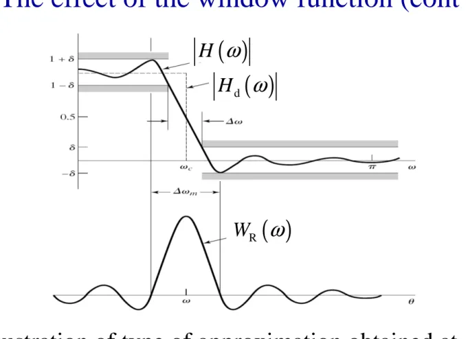
The effect of the window function (cont’)

( )

Hd ω

( )

H ω

( )

WR ω

Illustration of type of approximation obtained at

a discontinuity of the ideal frequency response.

The rectangular window

Main Lobe Width: 4π/(M+1) Sidelobe Magnitude= -13 db Stopband Attenuation=-21db

The rectangular window

( ) M=51

20 lg WR ω

Gibbs phenomena

( )

H ω ^H

( )

( )

H ω ^H

( )

Window functions for FIR filter design

• The Gibbs effect is alleviated by the use of windows that do not contain abrupt discontinuities in their time-domain characteristics w(n), and have correspondingly low sidelobes in their frequency- domain characteristics W( ω ).

• Some window functions that posses desirable Gibbs phenomena:

– Bartlett window – Hamming window – Hanning window – Blackman window – ...

Bartlett window

M=11

2 4 6 8 10

0 0.2 0.4 0.6 0.8 1

Amplitude

Time domain

0 0.2 0.4 0.6 0.8

-120 -100 -80 -60 -40 -20 0 20

Magnitude (dB)

Frequency domain

( ) ( ) ( )

B R R

W ω =W ω W ω ^wB

( )

( )

( )

( )

B

2 1 1 2

1 n M

w n

M

− −

= − −

Hanning window

M=11

2 4 6 8 10

0 0.2 0.4 0.6 0.8 1

Samples

Amplitude

Time domain

0 0.2 0.4 0.6 0.8

-80 -60 -40 -20 0 20

Normalized Frequency (×π rad/sample)

Magnitude (dB)

Frequency domain

( ) ( )

H R R R

4 4

1 1

W aW bW bW

M M

π π

ω = ω + ^ω − ^ + ^ω + ^

− −

   

( )

H

0.5 0.5cos 2

1 w n n

M

= − π

−

Hamming window

M=11

( ) ( )

H R R R

4 4

1 1

W aW bW bW

M M

π π

ω = ω + ^ω − ^ + ^ω + ^

− −

   

( )

H

0.54 0.46 cos 2

1 w n n

M

= − π

−

2 4 6 8 10

0 0.2 0.4 0.6 0.8 1

Amplitude

Time domain

0 0.2 0.4 0.6 0.8

-120 -100 -80 -60 -40 -20 0 20

Magnitude (dB)

Frequency domain

Blackman window

M=11 ( )

Bl

2 4

0.42 0.5cos 0.08cos

1 1

n n

w n

M M

π π

= − +

− −

2 4 6 8 10

0 0.2 0.4 0.6 0.8 1

Samples

Amplitude

Time domain

0 0.2 0.4 0.6 0.8

-140 -120 -100 -80 -60 -40 -20 0 20

Normalized Frequency (×π rad/sample)

Magnitude (dB)

Frequency domain

Important characteristics of some window functions

Window Type Peak Sidelobe Amplitude

(relative) [dB]

Approximate Width of Mainlobe

Peak

Approximation error 20 logδ

[dB]

Rectangular -13 4π/(M+1) -21

Bartlett -25 8π/(M+1) -25

Hanning -31 8π/(M+1) -44

Hamming -41 8π/(M+1) -53

Blackman -57 12π/(M+1) -74

Windows based FIR filter design

• Given δ

1

, δ

2

, ω

p

and ω

s

1. Compute

2. Compute 20lg( δ ) and select window type

3. Choose the filter order M, to meet transition width 4. Filter coefficients are given by

s

p

ω

ω ω

δ δ δ

−

=

∆

= min(

,

)

( )

( ) ( )

h n = h n w n

c 2

p s

ω

ω ω

( ) ( )

d d

1 2

h n H e

d

π ω

π

ω ω

π

= ∫ ^where

( )

2 g n h n M − 

=  − 

 

Implemetation on

FIR architecture

Pros and Cons of Window based Design

• Advantages

– Easy to design

– Can be applied to general linear system design

• Disadvantages

– Exceeds the specs everywhere except at the edges of the passband and stopband

– δ

1, δ

2, cannot be independently controlled. Have to design more conservatively for the smaller of the two.

:

Summary

• We developed the DFT by sampling the spectrum X(ω) of the sequence x(n).

• We developed the structure of the basic decimation-in-time FFT.

• Use of the FFT algorithm reduces the number of multiplications required to perform the DFT by a factor of more than 100 for 1024-point DFTs, with the advantage increasing with increasing DFT size.

• We have described the FIR filters design using windows. Historically, it was the first proposed method for FIR design. Its major disadvantage is the lack of precise control of design parameters.

• As a general rule, FIR filters are used in applications where there is a need for a linear-phase filter.

Next lecture: Adaptive signal processing