Neural Network-based Adaptive Sliding Mode Control Method for Tracking of a Nonholonomic Wheeled Mobile Robot with Unknown Wheel Slips, Model Uncertainties, and Unknown Bounded External Disturbances

(1)

Neural Network-based Adaptive Sliding Mode Control Method for Tracking of a

Nonholonomic Wheeled Mobile Robot with Unknown Wheel Slips, Model Uncertainties, and Unknown Bounded External Disturbances

Tinh Nguyen

¹

, Kiem Nguyentien

²

, Tuan Do

¹

, Tuan Pham

³

1Institute of Information Technology, Vietnam Academy of Science and Technology, Hoang Quoc Viet street 18, 100000 Hanoi, Vietnam e-mail: nvtinh@ioit.ac.vn; tuando@ioit.ac.vn

2Department of Electronics Power, Faculty of Electronics Engineering Technology, Hanoi University of Industry, Hanoi, Vietnam

e-mail: kiemnt@haui.edu.vn

3Space Technology Institute, Vietnam Academy of Science and Technology, Hoang Quoc Viet street 18, 100000 Hanoi, Vietnam, e-mail: pmtuan@sti.vast.vn

Abstract: This article represents a neural network-based adaptive sliding mode control (ASMC) method for tracking of a nonholonomic wheeled mobile robot (WMR) subject to unknown wheel slips, model uncertainties and unknown bounded disturbances. Self- recurrent wavelet neural networks (SRWNN) are employed in order to approximate unknown nonlinear functions due to the unknown wheel slips, model uncertainties, and unknown bounded external disturbances. By doing this, their harmful effects are compensated effectively. Thanks to this control method, a desired tracking performance of the closed-loop control system is achieved where the position tracking errors converge to an arbitrarily small neighborhood of the origin, regardless their initial values. According to Lyapunov theory and LaSalle extension, the stability of the whole closed-loop system is guaranteed to achieve the desired tracking performance. It is unnecessary to preliminarily offline train the neural network weights since they are easily initiated. Online tuning algorithms are established and used, for training the weights. Computer simulations are implemented to demonstrate the validity and efficiency of this proposed control method.

Keywords: Adaptive sliding mode control (ASMC); desired tracking performance; online tuning algorithm; unknown wheel slip; wheeled mobile robot (WMR)

(2)

1 Introduction

In recent years, control problems for wheeled mobile robots (WMR) are considered remarkable, due to their inherent nonlinear properties such as nonholonomic constraints and their wide applicability in various areas. Many researchers, all over the world, have paid attention to solving the tracking problems of WMRs by employing various techniques with the assumption “pure rolling without slip” being always satisfied. For example, an adaptive tracking controller in [1] employing a backstepping technique was developed for the dynamics of WMRs with unknown parameters. The content in [2] expressed a robust adaptive control method to cope with parametric uncertainties and external disturbances for nonholonomic WMRs. A wavelet-network-based control method was proposed in [3] for the dynamics of WMRs with unstructured unmodelled dynamics and unknown disturbance. Owing to having a fast response, good transient performance, and robustness against parameter variations, unstructured unmodelled dynamics, and unknown disturbances, the sliding mode control (SMC) technique has been applied widely for trajectory tracking problems of nonholonomic WMRs. For instance, the work in [4] proposed a tracking controller using the SMC technique for nonholonomic WMRs in polar coordinates. In addition, the authors in [5] also proposed an adaptive neural SMC method for trajectory tracking of nonholonomic WMRs with model uncertainties and external disturbances.

However, in practice, the assumption “pure rolling without slip” is often violated due to various factors such as slippery floor, external forces, and so on. The wheel slip is one of the reasons making the tracking performance of nonholonomic WMRs reduce considerably. Therefore, if one wants the tracking performance of the WMRs to be improved in such context, then control methods having the ability to overcome the undesired effects of the wheel slips must be taken into account.

Several research results have been published for trajectory tracking of nonholonomic WMRs subject to the wheel slips. In particular, an adaptive tracking control method by means of neural networks was proposed in [6] in order to overcome the harmful effect of the wheel slips. By employing gyro-sensors and encoders, the slip ratios were calculated in [7], [8]. Then the control approaches to compensate the wheel slips were proposed in these reports. The work in [9]

developed a robust controller dealing with not only slip-kinematics but also slip- dynamics by employing the framework of differential flatness. The authors in [10]

modeled overall the dynamics of a WMR subject to the wheel slips. Next, they proposed a discontinuous control technique for regulation control task and a SMC technique for sharp turning control task. The work in [11] proposed a feedback linearization control method for trajectory tracking of a WMR subject to both longitudinal and lateral slips between each driving wheel and the floor in an ideal condition where unknown bounded external disturbances, as well as, model

(3)

uncertainties did not exist. In addition, in this case, the values of the accelerations and velocities of the wheel slips could be measured precisely. On the contrary, such ideal condition barely exists in reality and it is difficult to exactly measure both the accelerations and the velocities of the wheel slips. Accordingly, it was impractical to employ this feedback linearization control method [11].

Therefore, most of these previous works assumed that the measurements of the wheel slips were made available by additional sensors such as global position systems (GPS), gyroscopes, accelerometers, etc. which are expensive and complex.

On the other hand, the neural network (NN) has been utilized as one of the intelligent techniques to enhance the performance of closed-loop control systems.

Unlike classification applications, the NN in feedback control application seems to be part of the closed-loop control system. For this reason, it is useful in order to have a NN closed-loop control system with on-line learning algorithms [12]

without the need of a preliminary off-line learning phase for the NN weights. In regard to the works in [5], [13], [14], and [15], the closed-loop control systems including self-recurrent wavelet neural networks (SRWNN) have been proposed.

In fact, the SRWNN is a combination of the properties of a recurrent neural network (RNN) [16], [17], namely the attractor dynamics, and the fast convergence of a wavelet neural network (WNN) [18], [19]. As a consequence, the SRWNN includes a mother wavelet layer comprising self-feedback neurons being able to not only capture the past information of the NN but also adapt sharply to quick changes of the control environment.

These above research results have motived us to propose a neural network-based ASMC method for trajectory tracking of a nonholonomic WMR in the presence of the unknown wheel slips, model uncertainties, and unknown bounded external disturbances. In this work, the proposed controller is based on the SRWNNs to compensate the unknown wheel slips, model uncertainties, and unknown bounded external disturbances. Furthermore, the measurements of the wheel slips are unnecessary. In sense of Lyapunov and LaSalle extension, on-line tuning algorithms for all the weights of the SRWNNs are derived. The uniformly ultimately bounded property of all the signals in the closed-loop control system is also assured.

This paper is organized as follows. In Section 2, the kinematics and dynamics of a nonholonomic WMR subjected to the unknown wheel slips as well as the structure of a SRWNN are briefly introduced. Section 3 expresses the problem statement and then proposes an ASMC method using SRWNNs, following which the stability of the whole closed-loop system is proven by using standard Lyapunov theory and LaSalle extension. Finally, computer simulations illustrate the validity and efficiency of the proposed control method in Section 4.

(4)

2 Preliminaries

2.1 Kinematics of the Nonholonomic WMR with the Unknown Wheel Slips

Let us take into account a nonholonomic WMR comprising two driving wheels and a caster wheel as shown in Figure 1.

To be specific, point G(x_G, y_G) is the center of mass of the WMR platform. Next, M(x_M, y_M) is the midpoint of the wheel shaft and chosen as the reference point of the WMR.  is the heading angle of the WMR. b expresses haft of the wheel shaft length. r illustrates the radius of each driving wheel. F₁ and F₂ reveal the total longitudinal friction forces at the right and left wheel, respectively. F₃ shows the totally lateral friction force along the wheel shaft. F₄ and  describe external force and moment acting at G, respectively.

When there is no wheel slip, the linear velocity and the yaw rate of the WMR, computed at M, are represented respectively as follows:

 

R L

2 2 r r

b

 



 

 

 

 

     

where  _R, _L denote the angular velocities of the right and left wheel about the wheel shaft, respectively.

Therefore, the kinematics of the WMR is written as follows:



Figure 1

A nonholonomic WMR subject to unknown wheel slips F₂

F1

F₃

 Left driving

wheel

Right driving wheel

caster wheel

a 2b

F₄





_L



_R

Wheel shaft

G M The

platform

θ

(5)

 ^M_M cos sin x

y



 

  

  

 



      

On the other hand, when the assumption of “pure rolling without slip” is violated, (1) and (2) are no longer true. Accordingly, let _R and_L be the coordinates of the longitudinal slip of the right and left wheels, respectively, and,  be the coordinate of the lateral slip along the wheel shaft (see Figure 1). In this case, the actual linear velocity of the WMR along the longitudinal direction is expressed in the following [11]:





R L



R L R L

2 2 2

r  ^    

         

The actual yaw rate of the WMR is computed as follows [11]:



R L



R L ,

2 2

r

b b

   

 ^  ^    with ^R ^L.

2b

 

 ^ (4) Thus, the kinematics of this WMR can be expressed in term of the coordinates of M as follows [11]:

 ^M_M cos sin

sin cos

x y

  

 

   

   

 



     (5)

Due to the wheel slips, the perturbed nonholonomic constrains can be written as follows [20]:

 _R  r_Rx_Mcosy_Msinb   (6)

 _L  r_Lx_Mcosy_Msinb   (7)

  x_Msiny_Mcos     (8)

2.2 Dynamics of the WMR with the Wheel Slips, the Model Uncertainties, and the Unknown Bounded External Disturbances

Let q



xG,yG, , ,     R, L, R, L



^T show a Lagrange coordinate vector. The nonholonomic constrains (6), (7), and (8) can be shown in the following form:

 A q q

 

0      (9)

(6)

where

 

^coscos ^sinsin ⁰0 0^{1 0}1 0 ⁰

sin cos 1 0 0 0 0

b r

a

 

 

 

 

   

  

 

A q 

The dynamic equation of the WMR can be represented as follows:

 Mqτd Nτ A q λ

 

^T     (10)

where λ



  1, 2, 3



^T is the vector of Lagrange multipliers to be considered as nonholonomic constraint forces. τ



 R, L



^T is the input vector with



_Rand



_L

being the torques at the right and left driving wheel about the wheel shaft, respectively. τ_d is a vector illustrating the model uncertainties such as the unstructured unmodelled dynamic components and the unknown bounded external disturbances such as the unknown external forces such as F₁, F₂, F₃, F₄,  (see Figure 1). N is the input transformation matrix shown as follows:

0 0 0 0 0 0 1 0 T

0 0 0 0 0 0 0 1

 

  

N .

Furthermore, it is easy to develop the following equation:

 qS q v₁

 

S₂

 

q γS q₃

 

    (11)

where v  _R, _L^T, γ



 R, L



^T,

T

1

cos sin sin cos 0 0 0 1 0

2 2 2 2 2

r ar r ar r

b b b

r ar r ar r

b b b

   

       

    

 

         

S

T

2

1 1 1

2 2 2 2 2

1 1 1 ,

2 2 2 2 2

a a

b b b

a a

b b b

   

       

    

 

          S

 

^T

3 sin cos 0 1 0 0 0 0 S

Subsequently, taking the time derivative of (11), we obtain:

           

1 1 2 2 3  3 

     

q S q v S q v S q γ S q γ S q S q  (12)

(7)

1 1

12 11

m m ,

m m

 

   

M S MS ₁^T ₂ ¹ ²

2 1

Q Q ,

Q Q

 

    Q S MS

T

1 3 G

1 , 2 1 m r

     

C S MS ₁^T ₃ _G ¹ ,

2 1 m ar

b

      G S MS

 

2 2 2 2

2

11 G 2 2 IG 2 ID W I ,W

4 4 4

r a r r

m m m r

b b

 

      

 

 

2 2 2 2

12 G 2 2 IG 2 ID

4 4 4

r a r r

m m

b b

 

    

  ,

 

2

1,2 G 1 2 IG 2 ID ,

4 4

r a r

Q m

b b

 

    

 

2 T

1 1 G

0 1 1 0 . 2

m ar

b ^ ^

   

B S MS  

The parameters of the WMR in the above matrices are illustrated in Table 1.

Table 1 The parameters of a WMR

Symbol QUANTITY Value

m_G The mass of the platform of the WMR 10 (kg)

I_G The inertial moment of the platform about the vertical

axis through point G. 4 (kg.m²)

a The distance between G and M (see Figure 1). 0.2 (m) C The distance between P and M (see Figure 3) 0.5 (m)

m_W The mass of each driving wheel 2 (kg)

I_W The inertial moment of each driving wheel about the

wheel shaft 0.1 (kg.m²)

ID

The inertial moment of each wheel about its diameter

axis 0.05 (kg.m²)

b Half-distance between two the wheels 0.3 (m)

r The radius of each driving wheel 0.15 (m)

(8)

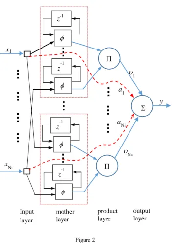
2.3 Structure of SRWNN

Let us use SRWNNs [5], [13], [14], [15] with structure as shown in Figure 2 including N_iinputs, one output, and N_iN_wavelets in the mother layer as an estimator to compensate the unknown wheel slips, model uncertainties, and unknown bounded external disturbances.

The structure of the SRWNNs comprises 4 layers: one input layer, a mother layer, a product layer, and one output layer. The output of each SRWNN is expressed as follows:



    ^{ }

1 1 1

i i

N

N N

j jk jk k k

j k k

y z N a x N

 

  

 













^{ } ^ ⁽¹⁴⁾

Here, the subscript jk reveals the k-th term of the j-th wavelet, N shows the number of iterations; the output y approximates an uncertainty; x_k reveals the k-th input; a_k seems to be a weight connecting the corresponding input to the output directly; _j illustrates the connection weight from the product nodes to the output node, and zjk

 

N x N

 

 jk jk



N ¹



jk^/jk^with_jk, _jk, and _jk corresponding to the translation factor, the dilation factor, and the weight of self- feedback loop, respectively. _jk



N1



describes the one-step recurrent term of

jk

 

N

 .

Besides, the mother wavelets are selected as jk

 

zjk  zjk^exp^¹₂z²jk^. In this work, all of a_k, _jk, _jk, _jk, and _j are trained online by using the on-line tuning algorithms to be discussed subsequently. For convenience, the vector of all the weights is defined in the following form:

 w a^T β^T ς^T ρ^T υ^T^T    (15)

with

T

1,..., ,...

k Ni

a a a

 

  

a  ^T ₁₁,..., ,...

jk N Ni _

  

 

  

β ς^T  ₁₁,...,_{N N}_i _

T

11,..., ,...

jk N Ni _

  

 

  

ρ υ^T  ₁,...,_j,...,_N_with1 k N_i1 j N_

(9)

Figure 2 Structure of SRWNN

3 Problem Statement and Designing the Adaptive Sliding Mode Control

3.1 Problem Statement

The control objective is to design the ASMC method using SRWNN for trajectory tracking of the WMR in the presence of the unknown wheel slips, the model uncertainties, and the unknown bounded external disturbances so that the point P of the WMR (see Figure 3) tracks the desired point D without measuring the accelerations and velocities of the wheel slips.

 z^-1

 x₁

x_Ni

y a1

aNi

₁

_N

Input layer

mother layer

product layer

output layer

 z^-1



(10)

Figure 3

The coordinate of the target is represented in the body coordinate system M-XY

D M

2

cos sin sin cos ,

x x y y

  

     

      

ζ    (16)

where



^x_D^,^y_D



is the position coordinates of D (see Figure 3).

Computing the second order derivative with respect to time of (16) yields

 ζ hv Ψ  ₁Ψ₂,     (17)

₁

2

x_D y_D

Y axis

C

x_M

D (target) P

M

X axis y_M

xP

O MY axis

MX axis yP

(11)

where

2 2

1 1

2 2

r r

b b

r r

b b

 

      

    

  

  

 

 

h , Ψ₁ and Ψ₂ are nonlinear components

revealed as follows:

D D D D

1

D D D D

cos sin sin cos

sin cos cos sin ,

x y x y

     

^ ^  ^  

 

      

Ψ hv with

 

2 ,

R L

r  

 ^

and ₂ ^D ^D

D D

sin cos

cos sin ,

x y

    

    

  

 

    

Ψ with

2

R L

 

 ^ ,

2

R L

 

 ^ .

Remark 2: Owing todet

 

1 ²

2 r

 b

 

h , if ₁≠ 0, then h in (17) is invertible.

Then, we define the vector of the position tracking errors as e =



e e1, 2



^T  ζ ζd, where ζ_d is the desired coordinate vector of the target D in M-XY. From the control objective mentioned in Sub-section 3.1 and Figure 3, one can easily express ζd 

 

C, 0^T.

A sliding surface is defined as follows:

 se + Λe      (18)

where Λ is a 22 diagonal, constant, positive definite matrix and can be chosen arbitrarily.

3.3 Structure of the Closed-Loop Control System

To begin with, let us propose the scheme of the whole closed-loop control system as shown in Figure 4.

Afterwards, since directly depending on the accelerations and velocities of the unknown wheel slips which are not measured in this work, Ψ₂ in (17) is unknown. Therefore, let us define an auxiliary variable which can be measured easily as follows:

 κ h ^¹



 ζd Λe Ψ 1



,     (19)

Alternatively, one can rewrite (13) as follows:

 Mv τ Bv d      (20)

(12)

where dQγ C Gτ_d shows all uncertainties because of the unknown wheel slips, the model uncertainties, and the unknown external disturbances

.

Figure 4

Scheme of the whole closed-loop control system

Adding Mκ to both of the sides of (20) and then combining the result with (17), (18), and (19) leads to

 Mh s^¹  τ Mκ Bv d Mh Ψ   ^¹ ₂   (21) Conversely, it is not easy to exactly know dynamic parameters of this WMR such as mass, moments of inertia, etc. Accordingly, it is impossible in order to precisely express all expressions consisting of these quantities. Therefore, one can show (21) in the following form:

 Mh sˆ ^¹  τ Mh s Mκ Bv d Mh Ψ^¹     ^¹ ₂,  (22)

where MM M ˆ withMˆ showing an approximation of M.

Remark 3: both M and Mˆ are always symmetric, invertible, positive definite matrices.

Multiplying both of the sides of (22) by hMˆ^¹ yields

 ^s^^{hM τ f x}^ˆ^¹ ^

 

^,^ ^ ^ ^ ^ ^(23)

where f x

 

hMˆ^¹Mh s Mκ Bv d Mh Ψ^¹     ^¹ 2, x v^T κ^T^T. Clearly, x can be measured easily.

Thanks to the strong capability of the SRWNN for approximating unknown nonlinear functions [5], [13], [14], [15], it can be employed in order to approximate f x

 

in (23) of the unknown wheel slips, the model uncertainties, and the unknown bounded external disturbances. By doing this, given a small

Controller

WMR subject to unknown wheel slip xM, yM, θ

Target

(xD, yD) ζd C, 0^T

e s

+

-

^{f x W}^ˆ

 

^ˆ

Equation (16)

ζ τ

SRWNN κ v

Equation (19)

s = e + Λe

Model uncertainties and unknown bounded external disturbances

Wheel slips

(13)

positive real number _M, there exists a vector of optimal weightsW^ w₁^^T w^{* T}₂ ^T such that:

 ^{f x}

 

^^{f x W}^ˆ



^



^^ε^ ^ ^ ^ ^ ^(24)

Here, x is used as the input of the SRWNN; ε is the vector of reconstruction errors and bounded by ε _M. Then, an estimation of ^{f x W}^ˆ



^



^{can be}

^ˆ ^^ε  (25)

Let ^{f x W}

 

be the functional deviation as follows:

^around^W^ˆ ^gives:

 ^{f x W}

   

^^{f W W}^ ^ˆ ^^O

 

^W ^ ^ ^ ^ ^(27)

with

   

*

* ˆ

ˆ 

 

 ^W ^W

f x W f W

W ^and ^O

 

^W denoting higher-order terms in Taylor series expansion.

Due to (25), (26), and (27), we can rewrite (23) as follows:

   

1 ˆ

ˆ ^ ˆ ' ˆ ,

   

s hM τ f x W f W W δ (28) where ^δ^^O

 

^W ^^ε^.

Now, we propose the control input employing the SRWNNs as follows:

 τ Mh^ ^ˆ ^¹^^Ks f x W^^ˆ

 

^ˆ ^    (29)

where K is a positive definition matrix and can be chosen arbitrarily.

(14)

Furthermore, the on-line tuning algorithms for all the weights are proposed as follows:

 ^W^ˆ ^{ }^_^f^'

 

^W^ˆ ^_^T^s^{ }^ ^{s W}^ˆ^,^ ^ ^ ^ ^(30)

where  and  are positive tuning gains and can be selected arbitrarily.

3.4 Stability

Assumption 1: the optimal weight vector W^ is bounded such that W^ W_M. It is worth noting that W_M is not used to perform the proposed controller. It is, however, just employed with the purpose of analyzing the stability of the entire closed-loop control system.

Assumption 2: all of x_D,y_D,x_D,y_D, x_D,and y_D are available and bounded.

Assumption 3: the accelerations and velocities of the unknown wheel slips are bounded.

Assumption 4: δin (28) is bounded such that δ b_ with b_ 0

Theorem 1: Let us consider the WMR subject to the unknown wheel slips, the model uncertainties, and the unknown bounded external disturbances with the kinematics (5) and the dynamics (13). If the control input using the SRWNN is proposed as (29), the weight vector is adjusted by (30), and Assumptions 1-4 are satisfied, then the errors, sand W, of the closed-loop control system as shown in Figure 4 are uniformly ultimately bounded and further s can be kept arbitrarily small.

Proof: Substitution of (29) into (28) results in the dynamics of the sliding vector as follows:

 ^s^{ }^{Ks f W W δ}^ ^'

 

^ˆ ^ ^{ } ^ ^ ^ ^(31)

By contrast, a Lyapunov candidate function is chosen as follows:

 1 ^T 1 ¹ ^T

2 2

V  s s ^W W     (32)

Taking the first derivative of V with time leads to

 Vs s^T  ^¹W W^T      (33)

Because of W Wˆ , substituting (30) and (31) into (33) achieves

(15)

^W^M ^W ^ ^W²



^ ^ ^(36)

here Kmin is the minimum singular value of K. Due to ^W^M ^W ^¹₂



^W^M



²^¹₂

 

^W ²^{we have}

 _min 1 ² 1 _M²

2 2 W

V   s ^K s   W b_   ^  (37) Observing (37) reveals that

V

is guaranteed to be negative definite as long as the term in the braces seems to be positive, that is, the following inequality is correct:

 _min 1 ² 1 _M²

2 2 W

K s   W b_      (38)

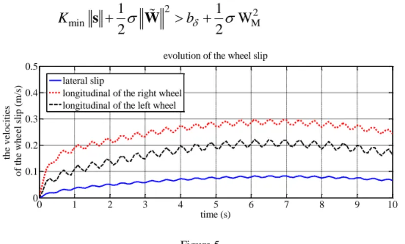
0 1 2 3 4 5 6 7 8 9 10

0 0.1 0.2 0.3 0.4 0.5

evolution of the wheel slip

time (s) the velocities of the wheel slip (m/s) lateral slip

longitudinal of the right wheel longitudinal of the left wheel

Figure 5 Evolution of the wheel slips

(16)

0 2 4 6 8 10 12 14 -2

-1 0 1 2 3 4

the comprison of tracking rerults

X axis (m)

Y axis (m)

desired trajectory

feedback linearization control method proposed control method

Figure 6

Comparison of tracking performances in Example 1

0 2 4 6 8 10

-2 -1 0 1 2

proposed control method

time (s)

position tracking errors (m)

0 2 4 6 8 10

-2 -1 0 1 2

time (s)

feedback linearization control method e1

e2

e1

e2

Figure 7

Comparison of position tracking errors in Example 1

0 1 2 3 4 5 6 7 8 9 10

0 50 100

the control inputs of the proposed control method

time (s)

control inputs (N.m)

torque R torque

L

Figure 8

Control inputs of the proposed control method in Example 1

(17)

As a consequence of this, according to Lyapunov theory and LaSalle extension, the error vectors, both s and W,are uniformly ultimately bounded in a compact set as follows:

 _min 1 ² 1 _M²

, W

2 2

K  b_ 

 

    

 

UB s W s W   (39)

As can be seen from (39), s can be kept as small as possible by increasing K_min suitably.

4 Simulation Results

In this section, computer simulations for trajectory tracking of the WMR were implemented to verify the correctness and effectiveness of the proposed control method. Moreover, a comparison between the tracking performance of this proposed control method and that of the feedback linearization control method [11] was executed to confirm the strong points of this proposed control method.

For comparison, both of the two methods were performed under the same condition that there existed the model uncertainties and the unknown bounded external disturbances, and the accelerations and velocities of the unknown wheel slips were not measured. Namely, without loss generality, it was assumed that

 

^T

d 3 sin(0.5 ), t 2.5 cos 0.4 t 

τ (N.m), and the unknown wheel slips

between the floor and the driving wheels are illustrated as Figure 5. Furthermore, the estimation of the matrix M was assumed as Mˆ 0.8M.

The control parameters were chosen as K = diag([6, 6]), Λ^diag



^[2, ^2]



. For simplicity, there was only one product node in each SRWNN. The weight tuning gains were set as  0.005, and  0.15. The initial values of the weight matrices were chosen to random numbers in [0, 1], other than that the weights of the self-feedback loops were chosen as 0. The initial posture of the WMR was assumed as x_P = C = 0.5 (m), y_P = 0 (m), and  = 0 (rad).

For illustration, two the following examples were carried out by Matlab/Simulink software.

Example 1: the target D was on a straight line with the following motion equation:

 ^D

D

4 , 2 0.5

x t

y t

  

   

 ^ ^ ^ ^ ^ ⁽⁴⁰⁾

Simulation results are shown in Figure 6, Figure 7, and Figure 8.

(18)

0 1 2 3 4 5 6 7 8 0

1 2 3 4

X axis (m)

Y axis (m)

comparison of two control methods

desired trajectory proposed controller

feedback linearization controller

Figure 9

Comparison of tracking performances in Example 2

0 5 10

0 0.5 1 1.5 2

proposed controller

time (s)

0 5 10

0 0.5 1 1.5 2

feedback linearization controller

time (s)

e1 e2

Figure 10

Comparison of position tracking errors in Example 2

0 1 2 3 4 5 6 7 8 9 10

-20 0 20 40 60 80

time (s)

control inputs (N.m)

the control inputs of the proposed control method

torque R torque

L

Figure 11

Control inputs of the proposed control method in Example 2

(19)

It is obvious from Figure 6 and Figure 7 that when the accelerations and velocities of the unknown wheel slips were not measured, and there existed the model uncertainties and the unknown bounded external disturbances; the approach in [11] could not overcome their undesired effects, whereas the proposed control method managed to effectively compensate the undesired effects. In addition, the control inputs of the latter were bounded as shown in Figure 8.

Example 2: the target D moved on a circular trajectory expressed as follows:



 

D D

5 3cos 0.25 , 2 3sin 0.25

x t

y t

  

  

 ^{ } ^ ^ ^ ⁽⁴¹⁾

The tracking performance is shown in Figure 9, Figure 10, and Figure 11.

Noticeably, regardless of the unknown wheel slips, the model uncertainties, and the unknown bounded disturbances, the proposed control method managed to compensate their effects very effectively whereas the approach in [11] could not.

Furthermore, the control inputs of the proposed method were bounded as illustrated in Figure 11.

It should also note that in Figure 7 and Figure 10 the position tracking errors of the proposed control method almost converged to zero, but that of the approach in [11] did not. In general, the tracking performance of the former is better than that of the latter in both the above examples.

It is clear that the vector of the position tracking errors, e in (18), converged to an arbitrarily small neighbourhood of the origin, thus, ₁ converged to an adjustable small neighbourhood of C. Consequently, according to Remark 2, one can easily conclude that h in (17), (19), (21), (22), and (29) is invertible.

From these simulation results, we can draw a conclusion that Theorem 1 is true and the proposed control method is robust against the unknown wheel slips, the model uncertainties, and the unknown bounded external disturbances.

Conclusion

In this work, an ASMC method based on SRWNN, with the online tuning algorithms has been developed, to allow the WMR to track a desired trajectory with the desired tracking performance, in the presence of the unknown wheel slips, model uncertainties and unknown bounded external disturbances. It is unnecessary for initial offline training for the weights of the SRWNN, since they can be initialized without difficulty. The online tuning algorithms are established from standard Lyapunov theory and LaSalle extension. It has been shown that not only the position tracking errors, but also, the neural network weight errors, are uniformly, ultimately bounded, via standard Lyapunov theory and LaSalle extension. The former can be kept arbitrarily small, by choosing the control gains appropriately. The results of the computer simulation confirmed the veracity and effectiveness of the proposed controller.

(20)

Acknowledgement

This work is supported by Vietnam Academy of Science and Technology under Grant VAST.01.06/17-18.

References

[1] T. Fukao, H. Nakagawa, and N. Adachi: Adaptive tracking control of a nonholonomic mobile robot, IEEE Trans. Robot. Automat., Vol. 16, No. 5, pp. 609-615, Oct. 2000

[2] M. S. Kim, J. H. Shin, S. G. Hong, and J. J. Lee: Designing a robust adaptive dynamic controller for nonholonomic mobile robots under modeling uncertainties and disturbances, Mechatronics, Vol. 13, No. 5, pp.

507-519, 2003

[3] D. Sousa, E. M. Hemerly, and R. K. H. Galvao: Adaptive control for mobile robot using wavelet networks, IEEE Trans. Syst., Man, Cybern. B, Cybern, Vol. 32, No. 4, pp. 493-504, Aug. 2002

[4] D. K. Chwa: Sliding-mode tracking control of nonholonomic wheeled mobile robots in polar coordinates, IEEE Trans. ControlSyst. Technol., Vol. 12, No. 4, pp. 637-644, Jul. 2004

[5] B. S. Park, S. J. Yoo, J. B. Park, and Y. H. Choi: Adaptive neural sliding mode control of nonholonomic wheeled mobile robots with model uncertainty, IEEE Trans. Control Syst. Technol., Vol 17, No. 1, pp. 207- 214, Jan. 2009

[6] H. Gao, X. Song, L. Ding, K. Xia, N. Li, Z. Deng: Adaptive motion control of wheeled mobile robot with unknown slippage,” Int. J. Control, Vol. 87, No. 8, pp. 1513-1522, Feb, 2014

[7] M. Seyr, S. Jakubek, Proprioceptive Navigation: Slip Estimation and Slip Control for Autonomous Wheeled Mobile Robots, in: Proc. RAM, Bangkok, Thailand, 2006, pp. 1-6

[8] L. Chang Boon, W. Danwei: Integrated Estimation for Wheeled Mobile Robot posture, velocities, and wheel skidding perturbations, in: Proc.

ICRA, Roma, Italy, 2007, pp. 2355-2360

[9] J.-C. Ryu, S.K. Agrawal: Differential flatness-based robust control of mobile robots in the presence of slip, Int. J. Robot. Res. Vol 30, pp. 463- 475, 2011

[10] Y. Tian, N. Sarkar: Control of a mobile robot subject to wheel slip,” J.

Intell. Robot. Syst., Vol. 74, pp. 915-929, 2014

[11] N. V. Tinh, N. T. Linh, P. T. Cat, P. M. Tuan, M. N. Anh, N. P. Anh:

Modeling and Feedback Linearization Control of a Nonholonomic Wheeled Mobile Robot with Longitudinal, Lateral Slips, In: Proc. CASE, Fort Worth, TX, USA., 2016, pp 996-1001

(21)

[12] F. L. Lewis, A. Yesildirek, and K. Liu: Multilayer neural-net robot controller with guaranteed tracking performance, IEEE Trans. Neural Networks, Vol. 7, pp. 1-12, 1996

[13] S. J. Yoo, Y. H. Choi, and J. B. Park: Generalized predictive control based on self-recurrent wavelet neural network for stable path tracking of mobile robots: Adaptive learning rate approach, IEEE Trans. Cir-cuit Syst. I, Reg.

Papers, Vol. 53, No. 6, pp. 1381-1394, Jun. 2006

[14] S. J. Yoo, J. B. Park, and Y. H. Choi: Adaptive dynamic surface control of flexible-joint robots using self-recurrent wavelet neural network, IEEE Trans. Syst., Man, Cybern. B, Cybern., Vol. 36, No. 6, pp. 1342-1355, Dec.

2006

[15] S. J. Yoo, J. B. Park, and Y. H. Choi: Indirect adaptive control of nonlinear dynamic systems using self recurrent wavelet neural network via adaptive learning rates, Inf. Sci., Vol. 177, No. 15, pp. 3074-3098, 2007

[16] C. C. Ku and K. Y. Lee: Diagonal recurrent neural networks for dy-namic systmes control, IEEE Trans. Neural Netw., Vol. 6, No. 1, pp. 144-156, Jan. 1995

[17] F. J. Lin, T. S. Lee, and C. H. Lin: Robust controller design with recurrent neural network for linear synchronous motor drive, IEEE Trans. Ind.

Electron., Vol. 50, No. 3, pp. 456-470, May/Jun. 2003

[18] B. Delyon, A. Juditsky, and A. Benveniste: Accuracy analysis for wavelet approximations, IEEE Trans. Neural Netw., Vol. 6, No. 2, pp. 332-348, Mar. 1995

[19] Y. Oussar, I. Rivals, L. Personnaz, and G. Dreyfus: Training wavelet networks for nonlinear dynamic input-output modeling, Neuro-comput., Vol. 20, pp. 173-188, 1998

[20] S. J. Yoo: Approximation-based adaptive control for a class of mobile robots with unknown skidding and slipping, Inter J Contr, Autom, Syst, Vol. 10, No. 4, pp. 703-710, 2012

[21] D. Wang and C. B. Low: Modeling and analysis of skidding and slipping in wheeled mobile robots: control design perspective, IEEE Trans. on Robotics, Vol. 24, No. 3, pp. 676-687, Jun, 2008

Neural Network-based Adaptive Sliding Mode Control Method for Tracking of a Nonholonomic Wheeled Mobile Robot with Unknown Wheel Slips, Model Uncertainties, and Unknown Bounded External Disturbances