Modeling Synchronization Problems: From Composed Petri Nets to Provable Linear Sequents
Ján Perháč, Daniel Mihályi, Valerie Novitzká
Department of Computers and Informatics, Faculty of Electrical Engineering and Informatics, Technical University of Košice, Letná 9 042 00 Košice, Slovakia Jan.Perhac@tuke.sk, Daniel.Mihalyi@tuke.sk, Valerie.Novitzka@tuke.sk
Abstract: Component-based programming has become a popular and frequently used method for software development, prepared from independent components by a composition. Our paper presents an illustration of how a composition of components can cause the emergence of new problems that should be solved, in order to obtain the desired results. We introduce a transformation of Petri nets to corresponding provable sequents of linear logic and then we show how a composition of simple Petri nets causes arising of synchronization problems. Transformation to provable linear sequents that ensures a verified behavior for such composed systems.
Keywords: linear logic; petri nets; component composition
1 Introduction
In the last decades, a new method of software development, a component-based programming, has become very popular. It can be characterized as a construction of program systems from working entities by their composition. There are many publications in the area of software engineering discussing basic principles of this method and providing practical guides for how to prepare such program systems, e.g. [21, 22, 23, 27, 29]. Among the basic properties of components is their independency, i.e. that they can be executed separately, can be reused, and should satisfy rules of composition (contracts and dependencies) to ensure that the whole system produces desired results. One of the important properties of a composition is that after it is composed, new problems can arise. The aim of our paper is to illustrate this situation on known examples of synchronization. We used two formal tools; Petri nets (PNs) and linear logic. Both tools are useful and frequently employed in modeling and behavioral description of program systems. We show how the behavior of PNs can be expressed by provable sequents of linear logic, and simultaneously, we show how the synchronization problems arise from the composition of simple components.
Petri nets are well-known mathematical and graphical tool for behavioral modeling of processes. They were designed especially for modeling systems with interacting concurrent processes [20, 30]. They are sometimes called place/transition nets and they enable graphical expression of the system execution.
Petri nets nowadays have a wide spectrum of applications, not only in concurrent programming, but also in business process modeling, data analysis, software design, simulation, and many others [2, 3, 9, 10]. The expressive power of Petri nets has been studied and compared with several other formal methods for the specification and description of systems. Such systems include algebraic specification in [24], which leads to the extension of the notion of tokens to structural ones, or with B-language [11], in which the transformation of Petri nets to B-language is defined for software development, from specification to implementation. In our paper we would like to present another correspondence, namely how PNs can be transform into provable linear logic sequents.
Linear logic is a logical system introduced by Jean-Yves Girard in 1987 [6, 7]. It enables description of processes as they behave in real world. It is capable of describing the dynamic of processes, parallelism, external and internal nondeterminism, consecutive processes, and it is also able to handle the resources on syntactic level. Thanks to these properties, linear logic can be considered as a bridge between computing science and logic [15]. Propositional linear logic is available for program systems description [1, 16], their behavior [26], and their extension with modal operators enables modeling of knowledge achievement [17, 18] mainly in intrusion detection systems to improve network reliability [28].
Linear logic has greater expressive power than classical logic, thanks to more connectives with special properties. Moreover, every formula of classical propositional logic can be expressed in linear logic. One of the most important properties of linear logic is its ability to describe the dynamic of processes. By linear implication it is possible to express sequentiality and causality of processes.
Another important property of linear logic is its ability to handle resources - logical space and logical time [14, 19]. It allows us to express the internal structure of the resources, their consumption, together with a continuation of processes in incremental time.
In our research, we were inspired by the approach published in [5], where PNs are defined as models of linear logic. The reverse property is in [13]. We follow up on this approach in a way by which each significant fragment of a PN can be described by a linear sequent. We formulate a transformation of Petri nets to provable linear sequents. To illustrate composition problems, we define a trivial working PN and show its behavior by corresponding provable linear sequent.
Composing two and five trivial PNs causes new problems to arise, namely synchronization problems of mutual exclusion, and deadlock. These problems are similar to the ones in the process of component composition in component-based systems. The examples of synchronization problems appear frequently in
textbooks or papers concerning with Petri nets [9, 11, 20, 25]. To illustrate the transformation from PNs to linear logic together with the appearance of synchronization problems in component composition, is our main aim that is not published yet in scientific publications.
2 Principles of Petri Nets
A Petri net is a known formal tool used mainly for modeling the behavior of concurrent systems as state-transition systems. Their advantage is that these models can be represented graphically, by directed bipartite graphs. A PN graph has two types of nodes: places and transitions. Places are represented by circles and transitions by arrows (arcs). Places express possible states of a system, and transitions represent changes of states, i.e. events. Places can contain special marks called tokens. A transition is enabled, i.e. it can be fired, if all places of input arcs contain required number of tokens. When a transition is fired, it produces tokens in all places on output arcs. Generally, execution of a PN is nondeterministic: when more than one transition is enabled, any of them can be fired. Any distribution of tokens over places represents a configuration of a given PN called marking. For any place p of a PN its marking is a function 𝑚: 𝑃 → ℕ0 returning a number of tokens in p. ℕ0 denotes the set of natural numbers with zero. A marking of a PN is defined as a tuple
𝑚 = (𝑚(𝑝1 ), … , 𝑚(𝑝𝑛)) (1)
of markings of all places in a PN.
A PN has two functions: pre and post. The 𝑝𝑟𝑒 function for each place and transition returns a number of arcs from a given place to a given transition. The 𝑝𝑜𝑠𝑡 function for each place and transition returns a number of arcs outgoing from a given transition to a given place. Formally, a Petri net is defined as a tuple
𝑃𝑁 = (𝑃, 𝑇, 𝑝𝑟𝑒, 𝑝𝑜𝑠𝑡, 𝑚0) , (2)
where 𝑃 = {𝑝1, … , 𝑝𝑛} is a finite set of places, 𝑇 = {𝑡1, … , 𝑡𝑛} is a finite set of transitions, 𝑝𝑟𝑒: 𝑃 × 𝑇 → ℕ0 and 𝑝𝑜𝑠𝑡: 𝑇 × 𝑃 → ℕ0 are pre- resp. post- conditions and 𝑚0 is initial marking before a PN starts its execution.
The execution of a PN is based on following two rules:
enabling rule formulates the condition under which a transition is allowed to be fired. A transition can be fired if each of its input places contains a number of tokens greater or equal than the given threshold
firing rule defines modification of a marking caused by firing a transition. When a transition 𝑡 is fired, a token from each input place is deleted, and to each output place a token is added
A behavior of a PN can be described as a sequence of markings reached during the execution of PN.
3 Basic Concepts of Linear Logic
Linear logic belongs to the new logical systems that are useful for describing and verifying of real systems. It facilitates the formulation of dynamic processes, nondeterminism, concurrency, and handling of resources such as time and space on syntactic level [12]. In this section we introduce the basic definitions of logical connectives and the deduction system of linear logic. Elementary propositions of linear logic can be considered as actions or resources.
Let 𝑃𝑟𝑜𝑝 = {𝑝1, 𝑝2, … } be a countable set of elementary propositions. In this paper we use the following syntax of linear formulas:
𝜑 ∷= 𝑝| 𝟏| 𝟎 |⊤| 𝜑 ⊗ 𝜓 | φ ⊕ ψ | 𝜑 & 𝜓 | 𝜑 𝜓 | 𝜑⊥ (3) where
𝜑 ⊗ 𝜑 is the multiplicative conjunction with neutral element 𝟏. This formula expresses that both actions perform simultaneously or both resources are available at once.
𝜑 & 𝜓 is the additive conjunction with neutral element ⊤. This formula expresses that only one of the actions performs, but we can deduce which one from the environment. Additive conjunction describes external nondeterminism.
𝜑 ⊕ 𝜑 is the additive disjunction with neutral element 𝟎. This formula expresses that only one of the actions performs but we cannot anticipate which one. Additive disjunction describes internal nondeterminism.
𝜑⊥ is the linear negation and it describes a reaction of an action 𝜑 or a consumption of a resource 𝜑. Linear negation has the property of involution, i.e. (𝜑⊥)⊥≡ 𝜑.
𝜑 𝜓 is the linear implication. This formula describes that the first action 𝜑 is a cause of the second (re)action 𝜓 or in the case of resources it expresses that the first resource is consumed after linear implication.
For linear formulas, we use sequent calculus. A sequent has the form
Γ├ 𝜑, (4)
that expresses that a formula 𝜑 is deducible from the formulas in the context Γ = 𝜑1, … , 𝜑𝑛 . The formulas on the left side of a sequent are assumptions, therefore we consider them as multiplicative conjunction ⊗. The formula 𝜑 on the right side is deducible from the assumptions.
The sequent deduction system consists of basic rules, rules for the connectives, rules for neutral elements and structural rules:
1. Basic rule:
𝜑 ⊢ 𝜑 (𝑖𝑑) 2. Rule for linear negation:
𝜑⊥≡ 𝜑 ⊥ (( )⊥) 3. Rules for neutral elements:
Γ ⊢ ⊤ (⊤−𝑟)
Γ, 0 ⊢ 𝜑 (0−𝑙) Γ ⊢ 𝜑
Γ, 1 ⊢ 𝜑 (1−𝑙)
⊢ 1 (1−𝑟)
4. Rules for connectives:
Γ1⊢ 𝜑1 Γ2, 𝜑2⊢ 𝜓
Γ1, 𝜑1 𝜑2, Γ2⊢ 𝜓 ( −𝑙) Γ, 𝜑1⊢ 𝜑2
Γ ⊢ 𝜑1 𝜑2 ( −𝑟) Γ, 𝜑1, 𝜑2⊢ 𝜓
Γ, 𝜑1⊗ 𝜑2⊢ 𝜓 (⊗−𝑙) Γ1⊢ 𝜑1 Γ2⊢ 𝜑2
Γ1, Γ2⊢ 𝜑1⊗ 𝜑2 (⊗−𝑟) Γ, 𝜑1⊢ 𝜓
Γ, 𝜑1 & 𝜑2⊢ 𝜓 (&−𝑙1) Γ, 𝜑2⊢ 𝜓
Γ, 𝜑1 & 𝜑2⊢ 𝜓 (&−𝑙2) Γ, 𝜑1⊢ 𝜓 Γ, 𝜑2⊢ 𝜓
Γ, 𝜑1 & 𝜑2⊢ 𝜓 (⊕−𝑙) Γ ⊢ 𝜑1 Γ ⊢ 𝜑2
Γ ⊢ 𝜑1 & 𝜑2 (&−𝑟) Γ, ⊢ 𝜑1
Γ ⊢ 𝜑1⊗ 𝜑2 (⊗−𝑟1) Γ ⊢ 𝜑2
Γ ⊢ 𝜑1⊗ 𝜑2 (⊗−𝑟2)
5. Structural rules:
Γ, 𝜑1, 𝜑2⊢ 𝜓
Γ, 𝜑2, 𝜑1⊢ 𝜓 (𝑒𝑥𝑐ℎ) Γ1⊢ 𝜑 Γ2⊢ 𝜑
Γ1, Γ2⊢ 𝜓 (⊗−𝑟) The basic rule is the axiom of identity, linear negation is expressed as linear implication. The rules of connectives introduce connectives on the left or on the right part of a sequent. The only structural rules are exchange and cut rules. We note that in linear logic it is important which resources and how many of them we have. Therefore, the obvious structural rules of weakening and contraction are not allowed, only in controlled way using special unary connectives, exponentials. In this paper, we do not use exponentials; their definition together with
corresponding deduction rules is in [8]. A proof in sequent calculus is a tree, where the root is a proven sequent, and every step is the application of an appropriate deduction rule. A sequent is provable if all of the leaves of its proof tree are identities.
4 Transformation of Petri Net Patterns to Linear Logic Sequents
In this section we define transformations of some parts, the patterns of PNs, to the corresponding linear formulas. We select several significant patterns that occur in synchronization PNs and we define corresponding linear logic sequents. All other patterns can be transformed similarly using this idea.
We introduce the following notation. A place 𝑝 of a PN containing one token, i.e.
with the marking 𝑚(𝑝) = 1, we denote by the elementary proposition 𝑝 of linear logic. Marking expressing that a place 𝑝1 contains one token and a place 𝑝2 contains two tokens, can be denoted using multiplicative conjunction:
𝑝1⊗ 𝑝2⊗ 𝑝2 (5)
For describing of a PN transition by linear formula we use linear implication .
The premise of the implication is a marking that makes a transition 𝑡 to be enabled and the conclusion is the marking that arises after firing of 𝑡. Linear implication expresses change of a state, caused by firing a transition together with the consumed resources (tokens) on the left side and the produced resources (tokens) on the right side of implication [4]. For instance, if 𝑡 is a transition enabled when the places 𝑝1 and 𝑝2 have both one token and after firing 𝑡 the place 𝑝3 obtains a token, then this transition can be denoted by the following linear implication:
𝑡 ≡ 𝑝1 ⊗ 𝑝2 𝑝3 (6)
A behavior of a PN is described by the sequents of linear logic in the form:
𝑚, 𝑙 ├ 𝑚′, (7)
where
𝑚 is a marking before firing a transition
𝑙 is a list of enabled transitions expressed by linear implications defined above
𝑚′ is a marking after firing a transition
Such sequents express that the marking 𝑚′ is produced from a marking 𝑚 by firing a transition from 𝑙.
Now, we consider the characteristic fragments of PNs representing their possible structure and we formulate the corresponding linear formulas and sequents.
Precisely:
places of a PN are transformed into linear formulas
transitions of a PN are transformed into linear implications
We choose a sequence illustrated in Figure 1 as the first pattern. The transition 𝑡 is enabled if the place 𝑝1 contains at least one token. After firing 𝑡, the place 𝑝2
obtains one token.
Figure 1 Sequence
This pattern can be transformed to the following sequent:
𝑝1, 𝑡├ 𝑝2, (8)
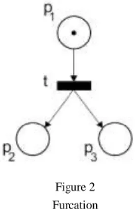
where 𝑡 ≡ 𝑝1 𝑝2. We call this sequent causality, because 𝑝1 is a cause of 𝑝2. The pattern in Figure2 depicts a situation of furcation:
Figure 2 Furcation
This pattern has one transition 𝑡 that is enabled if at least one token is in 𝑝1. Firing of 𝑡 produces one token in both 𝑝2 and 𝑝3, simultaneously. Therefore, the corresponding sequent expresses concurrency:
𝑝1, 𝑡├ 𝑝2⊗ 𝑝3 (9)
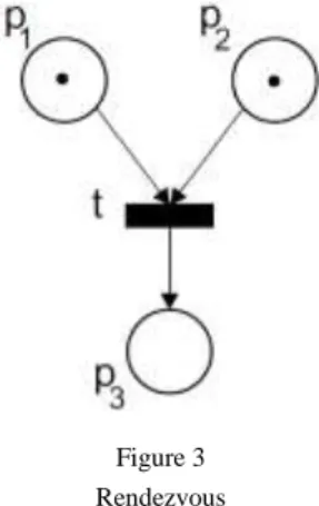
The pattern in Figure 3 illustrates a situation of rendezvous. To be 𝑡 enabled the places 𝑝1 and 𝑝2 have to have a token and after firing 𝑡 one token is produced in 𝑝3.
Figure 3 Rendezvous
We transform this pattern to the following sequent expressing synchronization:
𝑝1, 𝑝2, 𝑡├ 𝑝3 (10)
Up to now, all patterns were deterministic because they have only one enabled transition.
The next two patterns express nondeterministic behavior. The first of them in Figure4 is free choice. Either 𝑡1 or 𝑡2 are enabled but we cannot decide which of them.
Figure 4 Free choice
We transform this pattern to the sequent using additive disjunction ⊕ between formulas describing enabled transitions on the left side, because only one of 𝑡1 or 𝑡2 can be fired, but we do not know which one. It expresses internal nondeterminism. Producing tokens on the right side is expressed by linear formula by additive conjunction because a token can be obtained either in 𝑝2 or in 𝑝3
depending on previous action:
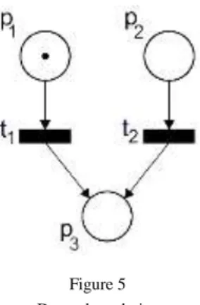
𝑝1, 𝑡1⊕ 𝑡2├ 𝑝2& 𝑝3. (11) The last pattern that we consider is dependent choice in Figure5. Dependent or environmental choice expresses the situation when only one transition of 𝑡1 or 𝑡2
can be fired, but it depends on the occurence of a token either in 𝑝1 or in 𝑝2. In the other words, this choice depends on the given environment. Firing any of transition 𝑡1 or 𝑡2 produces one token in the place 𝑝3.
Figure 5 Dependent choice
We transform this pattern to the linear sequent with additive conjunction describing transitions on the left side, because firing of 𝑡1 or 𝑡2 depends on the situation in 𝑝1 or 𝑝2, respectively:
𝑝1 & 𝑝2, 𝑡1 & 𝑡2├ 𝑝3 (12)
5 Synchronization Problems Arising from PNs Composition and Verifying by Proofs
In this section, we present the main aim of our paper. First, we define a trivial PN that works, i.e. its transitions can be enabled and fired. Considering a trivial PN as a component, when we compose two such PNs a new problem arises, that is known as mutual exclusion. We transform such composed PN into linear sequent and verify it by a proof. Second, we compose five trivial PNs that lead to arising of a known case of dining philosophers, i.e. deadlock problem. Again, we transform this composed PN into linear sequent and verify it by a proof. To summarize, we illustrate not only transformation of PNs to corresponding linear sequents, but also that composition of components together can cause arising of new problems that have to be solved in order to reach desired system behavior.
We start with a trivial PN in Figure 6. It is clear that this PN works and its behavior is deterministic. With a little imagination, we can call this PN, a dining philosopher.
Figure 6 A dining philosopher
This trivial PN consists of three places, where 𝑓1 and 𝑓2 represent forks and 𝑝1𝑒
represents an eating philosopher. This PN has two transitions 𝑡1𝑒 and 𝑡1𝑓 and its initial marking is 𝑚0= (1,0,1). If both forks 𝑓1 and 𝑓2 are available, i.e. both corresponding places have a token, the transition 𝑡1𝑓 is enabled and after firing, the place 𝑝1𝑒 obtains a token, i.e. the philosopher is eating. In this state the transition 𝑡1𝑓 is enabled and after firing, the philosopher releases the forks and starts to think.
The behavior of this PN can be expressed by the linear sequent:
𝑓2, 𝑓1, (𝑓2⊗ 𝑓1) 𝑝1𝑒, 𝑝1𝑒(𝑓2⊗ 𝑓1) ├ 𝑓2⊗ 𝑓1 (13) with the following proof in the Figure 7:
Figure 7 Proof of dining philosopher
Now we consider the previous PN in Figure6 as a component. By composing two such components (Fig. 8), we get the well-known problem of mutual exclusion (mutex). The interaction between the components is represented by the place 𝑓2. The principle of mutex is that only one of the processes can be executed in one moment, in other words, if one philosopher is eating (i.e. he possesses his left and right forks), the second is thinking and vice versa. Let the initial marking of this PN be 𝑚0= (1,0,1,0,1).
Figure 8 Mutual exclusion There are two possibilities how this PN works:
either 𝑡2𝑓 is fired, which corresponds to the linear logic sequent:
𝑓3, 𝑓2, 𝑓1, (𝑓3⊗ 𝑓2) 𝑝2𝑒├ 𝑝2𝑒⊗ 𝑓1 (14)
or 𝑡1𝑓 is fired, this case is expressed by linear logic sequent:
𝑓3, 𝑓2, 𝑓1, (𝑓2⊗ 𝑓1) 𝑝1𝑒├ 𝑝1𝑒⊗ 𝑓3 (15) The behavior of mutex can be described by the following linear logic sequent:
𝑓3, 𝑓2, 𝑓1, ((𝑓2⊗ 𝑓1) 𝑝1𝑒) ⊕ ((𝑓3⊗ 𝑓2) 𝑝2𝑒)├(𝑝1𝑒⊗ 𝑓3)&(𝑝2𝑒⊗ 𝑓1),
where we use internal nondeterminism on the left side, i.e. additive disjunction ⊕ between transitions 𝑡2𝑓 and 𝑡1𝑓. On the right side of this sequent, we use additive conjunction & between tokens, because they depend on which of the transitions 𝑡2𝑓 and 𝑡1𝑓 was actually fired. This sequent is provable and we present a left branch of this proof tree depicted in the Figure 9.
Figure 9 Proof of mutual exclusion
The right branch of the proof tree can be constructed similarly. Provability of this sequent ensures that we have a solution of mutual exclusion.
Now, we compose five trivial PNs (components) together and here a new problem arises, known as the problem of five dining philosophers, i.e. deadlock problem (Figure10).
Figure 10
Problem of five dining philosophers
If we assume the order of places 𝑝1𝑒, 𝑝2𝑒, 𝑝3𝑒, 𝑝4𝑒, 𝑝5𝑒, 𝑓1, 𝑓2, 𝑓3, 𝑓4, 𝑓5, then the initial marking is 𝑚0= (0, 0, 0, 0, 0, 1, 1, 1, 1, 1). If a place 𝑝𝑖, 𝑖 = 1, … , 5 has a token, the philosopher 𝑖 is eating, if it is empty, he is thinking. The places 𝑓1, 𝑓2, 𝑓3, 𝑓4, 𝑓5 serve for forks, the places 𝑝1𝑒, 𝑝2𝑒, 𝑝3𝑒, 𝑝4𝑒, 𝑝5𝑒 mean that corresponding philosophers eat.
This system works if every philosopher can eat, i.e. each process in a system can be executed. The problem occurs, when each philosopher takes its right fork and then they are waiting forever for the second fork; or in other words, if each process needs a certain resource to be executed, but any of them cannot release resources before finishing their execution. This problem is known as deadlock.
From the previous ideas it is clear that either one philosopher can eat, or two not neighbor philosophers can eat at one moment. We describe one of the possible solutions of this problem.
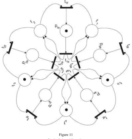
Consider that in the first step one philosopher, e.g. 𝑝1𝑒 is eating. That means, he takes both forks 𝑓1 and 𝑓2 and the transition 𝑡1𝑓 is fired. Figure11 illustrates the system after firing 𝑡1𝑓.
Figure 11 Single dining philosopher We describe this action by the linear sequent
𝑓1, 𝑓2, 𝑓3, 𝑓4, 𝑓5, 𝑓1⊗ 𝑓2 𝑝1𝑒├ 𝑓5⊗ (𝑓4⊗ (𝑝1𝑒⊗ 𝑓3)) (16) together with its (fragment of) proof depicted in the Figure 12:
Figure 12
Proof of single dining philosopher sequent
We again omit the left branches of this proof consisting of identities 𝑓5├ 𝑓5 and 𝑓4├ 𝑓4.
After finishing his work (eating), 𝑝1𝑒 releases both forks, i.e. 𝑡1𝑒 is fired and we get the initial marking of PN, which is described by the sequent:
𝑓3, 𝑓4, 𝑓5, 𝑝1𝑒, 𝑝1𝑒 (𝑓2⊗ 𝑓1)├ 𝑓5⊗ (𝑓4⊗ (𝑓3⊗ (𝑓2⊗ 𝑓1))), (17) and proven by the following (fragment of) proof in Figure 13:
Figure 13
Proof of single dining philosopher after finishing work
Again, the missing left branches of the proof denoted by … contain identities for 𝑓5, 𝑓4 and 𝑓3.
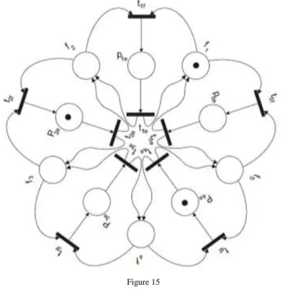
The second step is to enable two philosophers, e.g. 𝑝2 and 𝑝4, to eat as it is in Figure 15. In this step two transitions 𝑡2𝑓 and 𝑡4𝑓 can be fired simultaneously, because 𝑝2𝑒 and 𝑝4𝑒 have available both forks 𝑓2, 𝑓3 and 𝑓4, 𝑓5, respectively.
The corresponding linear logic formula:
𝑓1, 𝑓2, 𝑓3, 𝑓4, 𝑓5, (𝑓3⊗ 𝑓2 𝑝2𝑒) ⊗ (𝑓5⊗ 𝑓4 𝑝4𝑒)├ 𝑓1⊗ (𝑝4𝑒⊗ 𝑝2𝑒),(18) and its proof can be constructed in similar way as the proofs above depicted in Figure 14.
Figure 14
Proof of two dining philosophers
After finishing their dinner, the philosophers 𝑝2𝑒 and 𝑝4𝑒 release their forks, i.e.
the transition 𝑡2𝑒 and 𝑡4𝑒 are fired simultaneously. The corresponding linear logic sequent and its proof can be constructed as above.
As the last step we consider that remaining philosophers 𝑝3 and 𝑝5 will eat. The corresponding linear sequent and its proof can be constructed similarly as in the previous steps. Now we have the solution of PN, because all philosophers had their dinner and we translated the behavior into corresponding provable linear sequents.
Figure 15 Two dining philosophers
Conclusions
In this paper, we presented an illustration on how the actual problem of component composition, used in component-based systems, can cause the advent of new problems. These problems need to be identified and solved. For achieving this aim, we apply a method of Petri nets transformation to the corresponding provable linear sequents. The proofs of constructed sequents ensure the correctness, they can be used as a specification of a system and they can help in achieving reliable software products. In our examples, we are concerned with only one kind of such problems, namely synchronization problems of mutual exclusion and deadlock that appear after the compositions of trivial working Petri nets. Our approach enables to formulate the solutions by corresponding provable sequents.
We hope that our approach can be useful for education purposes, because it is simple, uses known concepts of PNs and linear logic, and is illustrative to comprehend component composition.
There are several open problems and possible ideas for solving them, by extending our approach. One of the advantages of linear logic is its resource character. First, we would like to formulate a transformation of timed Petri nets to linear formulas using polarization and focalization of the proof steps enabling to express time incrementally. After further study of Girard’s theory of Ludics and its handling another resource, a space, we would like to transform explicit information about data types in colored Petri nets to linear logic proofs.
It is a challenge for us to work out our approach also for colored Petri nets, i.e. to define transformation from Petri nets, to the sequents of linear logic and illustrate it on significant examples.
The main result of our work is a systematically, worked out solution, for practical programmers, respectively, for students, on how different various known formal tools can be combined and proved, together with an illustration of component composition.
References
[1] Abramsky S.: Computational interpretations of linear logic, Technical Report 90/20, Department of Computing, Imperial College, London, pp. 1- 15, 1990
[2] Aalst W. M. P., van der, Hee, K. M., van: Workflow management: models, methods, and systems, MIT Press, Cambridge, MA, 2002
[3] Aalst W. M. P., van der: The application of Petri nets to workflow management, J. of Circuits, Systems and Computations 8 (1), pp. 21-66, 1998
[4] Demeterová, E., Mihályi, D., Novitzká, V.: Component composition using linear logic and Petri nets, proceedings of the IEEE 2015 International Scientific Conference on Informatics, Poprad, pp. 91-96, 2015
[5] Engberg U., Glynn W.: Petri nets as models of linear logic, LNCS 431, pp.
147-161, 1990
[6] Girard J.-Y.: Linear logic, Theoretical Computer Science, Vol. 50, pp. 1- 102, 1987
[7] Girard J.-Y.: Linear logic: Its syntax and semantics, Cambridge University Press, 2003
[8] Girard J.-Y., Taylor P., Lafont Y.: Proofs and types, Cambridge University Press, New York, NY, USA, 1989
[9] Girault C., Valk R.: Petri nets for systems engineering - a guide to modeling, verification, and applications, Springer, 2003
[10] Korečko, Š., Marcinčin, J., Slodičák, V.: A tool for management of networked simulations, Lecture Notes in Computer Science: Application and Theory of Petri Nets. Vol. 7347, pp. 408-417, 2012
[11] Korečko, Š., Sobota, B.: Petri nets to B-language transformation in software development, Acta Polytechnica Hungarica Vol. 11, No. 6, pp.
187-206, 2014
[12] Lincoln P.: Linear logic, SRI and Stanford University, 1992
[13] Martí-Oliet, N., Meseguer, J.: From Petri Nets to Linear Logics through Categories: A survey, World Scientific Publishing Company, International Journal of Foundations of Computer Science, Vol. 2, No. 4, pp. 297-399, 1991
[14] Novitzká V., Mihályi D.: Resource-oriented programming based on linear logic, Acta Polytechnica Hungarica, Vol. 4, No. 2, 2007, pp. 157-166 [15] Mihályi D., Novitzká V.: What about linear logic in computer science?,
Department of Computers and Informatics, Technical University of Košice, Acta Polytechnica Hungarica, Vol.~10, No. 4, 2013, pp. 147-160
[16] Novitzká V. Mihályi D., Slodičák V.: Linear logical reasoning on programming, Acta Electrotechnica et Informatica, No. 3, Vol. 6, pp. 34- 39, 2006
[17] Mihályi D., Novitzká V., Towards the knowledge in coalgebraic model of IDS, Computing and Informatics, Vol. 33, No. 1, 2014, pp. 61-78
[18] Perháč J., Mihályi D., Novitzká V.: Between syntax and semantics of resource oriented logic for IDS behavior description, Journal of Applied Mathematics and Computational Mechanics. Vol. 15, No. 2, pp. 105-118, 2016
[19] Perháč J., Mihályi D.: Intrusion Detection System Behavior as Resource- Oriented Formula, Acta Electrotechnica et Informatica. Roč. 15, No. 3, pp.
9-13, 2015
[20] Peterson, James L.: Petri theory and the modeling of systems, Englewood Cliffs, N.J.: Prentice-Hall, 1981
[21] Pietriková, E., Chodarev, S. Profile-driven source code exploration Proceedings of the 2015 Federated Conference on Computer Science and Information Systems, FedCSIS 2015: Lodz, Poland, pp. 929-934, 2015 [22] Polberger, D.: Component technology in an embedded system, Lund
University, USA, 2009
[23] Raclet, J. B.: A modal interface theory for component-based design, Fundam. Informatics, Vol. 108, No. 1-2, 2011, pp.119-149
[24] Reisig, W.: Petri nets and algebraic specifications, Theoretical Computer Science 80 (1), pp. 1-34, 1991
[25] Riemann, R. C.: Structural and Semantical Methods in the High Level Petri Net Calculus, Herbert Utz Verlag, 1999
[26] Slodičák, V., Macko, P.: The role of linear logic in coalgebraical approach of computing, Journal of Information and Organizational Sciences. Vol. 35, No. 2, pp. 197-213, 2011
[27] Szyperski, C., Gruntz, D., Murer, S.: Component software beyond object- oriented programming, ACM Press, New York, 2002
[28] Vokorokos, L., Adám, N.: Secure web server system resources utilization, Acta Polytechnica Hungarica Vol. 12, No. 2, pp. 5-19, 2015
[29] Wang, A., Qian, K.: Component-oriented programming, Wiley- Interscience, 2005
[30] Winskel, G., Nielsen, M.: Models of Concurrency, In: Handbook of Logic and the Foundation of Computer Science, Vol. 4, 1993, pp.1-148