CORVINUS UNIVERSITY OF BUDAPEST
DEPARTMENT OF MATHEMATICAL ECONOMICS AND ECONOMIC ANALYSIS Fővám tér 8., 1093 Budapest, Hungary Phone: (+36-1) 482-5541, 482-5155 Fax: (+36-1) 482-5029 Email: zsolt.darvas@uni-corvinus.hu
W ORKING P APER
2005 / 4
F ISCAL D IVERGENCE AND B USINESS C YCLE
S YNCHRONIZATION : I RRESPONSIBILITY IS I DIOSYNCRATIC
Zsolt Darvas, Andrew K. Rose and György Szapáry
Budapest, 2005.
Fiscal Divergence and Business Cycle Synchronization:
Irresponsibility is Idiosyncratic
Zsolt Darvas, Andrew K. Rose and György Szapáry*
Draft Revised as of: August 9, 2005 Abstract
Using a panel of 21 OECD countries and 40 years of annual data, we find that countries with similar government budget positions tend to have business cycles that fluctuate more closely. That is, fiscal convergence (in the form of persistently similar ratios of government surplus/deficit to GDP) is systematically associated with more synchronized business cycles. We also find evidence that reduced fiscal deficits increase business cycle synchronization. The Maastricht “convergence criteria,” used to determine eligibility for EMU, encouraged fiscal convergence and deficit reduction. They may thus have indirectly moved Europe closer to an optimum currency area, by reducing countries’ abilities to create idiosyncratic fiscal shocks. Our empirical results are economically and statistically significant, and robust.
Keywords: European; monetary; union; policy; Maastricht; criteria; optimum; Mundell.
JEL Classification Numbers: F42
Zsolt Darvas Andrew K. Rose György Szapáry
Fővám tér 8 Haas School of Business Szabadság tér 8-9 Corvinus University University of California Magyar Nemzeti Bank H-1093 Budapest, Hungary Berkeley, CA USA 94720-1900 H-1850 Budapest Hungary Tel: +36 (1) 482-5279 +1 (510) 642-6609 +36 (1) 428 2770
Fax: +36 (1) 482-5029 +1 (510) 642-4700 +36 (1) 428 2581 zsolt.darvas@uni-corvinus.hu arose@haas.berkeley.edu szaparygy@mnb.hu
* Darvas is Assistant Professor, Department of Mathematical Economics and Economic Analysis, Corvinus University. Rose is B.T. Rocca Jr. Professor of International Trade and Economic Analysis and Policy in the Haas School of Business at the University of California, Berkeley, NBER research associate and CEPR Research Fellow. Szapáry is deputy governor of the Magyar Nemzeti Bank. The idea of this paper stemmed from a conversation with Miriam Green. Rose thanks the Banco de España for hospitality during the course of this research. For comments we thank: Dave Backus, Fabrizio Balassone, Marianne Baxter, Péter Benczúr, Helge Berger, Paul de Grauwe, Antonio Fatás, Jon Faust, Jeff Frankel, Joe Gagnon, Francesco Giavazzi, Linda Goldberg, Jim Harrigan, Dale Henderson, Zoltán Jakab, Olivier Jeanne, Sebnem Kalemli-Ozcan, Pat Kehoe, Phil Lane, Jacques Melitz, Roberto Perotti, Paolo Pesenti, Lucrezia Reichlin, Roberto Rigobon, John Rogers, Eric van Wincoop, Charles Wyplosz, and seminar participants at ISOM 2005, the Bundesbank, the Federal Reserve Bank of New York, the Federal Reserve Board, the International Monetary Fund, the Magyar Nemzeti Bank, and the National Bank of Poland. The views expressed below do not necessarily represent those of the Magyar Nemzeti Bank or its staff. A current version of this paper, key output, and the data set used in the paper are available at http://faculty.haas.berkeley.edu/arose and at http://www.uni-corvinus.hu/darvas .
1. Introduction
In 1998, European countries qualified for entry into European Monetary Union (EMU) on the basis of five “convergence criteria.” The criteria were enshrined in the 1992 Maastricht Treaty and quantify targets concerning inflation, long-term bond yields, exchange rates, government debt, and the government budget. The Maastricht convergence criteria are of more than of historical relevance, since they will also be applied to future EMU entrants. Further, the 1997 “Stability and Growth Pact” implies that the fiscal criteria are still, in principle, binding.1
Most economists – particularly non-Europeans – view the Maastricht convergence criteria with skepticism. The reason is simple: they have little to do with standard economic arguments concerning “optimal currency areas,” monetary unions that are desirable and sustainable. The consensus in economics is that from a theoretical viewpoint, monetary unions make sense for countries with synchronized business cycles, integrated markets, flexibility, and mechanisms to share risk. The overlap between the Maastricht convergence criteria and the optimum currency area criteria is small.2
Clearly the direct correspondence between the (Maastricht) criteria actually applied for EMU entry and the appropriate (optimum currency area) criteria is poor. In this paper we ask if there is an indirect connection. We focus on the most controversial Maastricht criteria – the total government budget deficit/GDP ratio – and link it empirically to arguably the most important optimum currency area criterion, namely the synchronization of business cycles. Using a panel of data that includes twenty-one countries and forty years of data, we show that countries with divergent fiscal policies (i.e., large average cross-country differences in the ratio of general government net lending/borrowing to GDP) tend to have less synchronized business cycles. We estimate that each percentage point of fiscal divergence between a pair of countries tends to lower the correlation coefficient of their business cycles by between .03 and .12. This effect is both statistically and economically significant. We also show that reduced levels of primary fiscal deficits (or increased primary surpluses) tend to increase the level of business cycle synchronization, though the evidence for this effect is somewhat weaker.
A concrete example may clarify things. When the Maastricht Treaty was signed in 1992, the total Italian budget deficit was 10.7% of GDP, and had been hovering at or above 11% of GDP for a decade. This was in sharp contrast to the typical German deficit, which was 2.6% of GDP in 1992.3 The drive to enter EMU – that is, to satisfy the Maastricht criteria – encouraged this gap to shrink by around eight percentage points; by the 1999 start, Italy’s budget deficit had fallen to 1.7%, similar to the German deficit of 1.5%. In this paper, we ask: could such fiscal convergence have an effect on the synchronization of business cycles between Germany and Italy?
1 In EU terminology, EMU technically refers to Economic and Monetary Union, which is different from the euro area. All EU countries are members of the Economic and Monetary Union, but only twelve members are currently members of the euro area. In the academic literature, EMU generally refers to the European monetary union. In this paper we follow conventional practice and use EMU to refer to the euro area.
2 We ignore the design of monetary institutions and policies for the time being. These are relevant to both the Maastricht Treaty and Optimum Currency Area considerations, but are not intrinsically either national or international. In any case, there is considerable overlap between the two sets of criteria in this respect.
3 Table 7A of “Cyclical Adjustment of Budget Balances” produced by ECFIN, EC, Spring 2005, available at http://europa.eu.int/comm/economy_finance/indicators/general_government_data/2005/cabb_spring2005en.
Alternatively, the (cross-country) standard deviation of the government budget position/GDP ratio was 4.1% for the EURO-12 in 1991, and only 2.1% in 1999; did this convergence in fiscal positions affect business cycle synchronization at the start of EMU?4 We find that the answer is generally positive; a larger panel of OECD data indicates that fiscal convergence (in either the total or primary budget balance) is systematically associated with more synchronized economic activity.
Whether or not it was intentional, the application of the Maastricht convergence criteria may have moved the EMU entrants closer to being an optimum currency area, since fiscal convergence tends to synchronize business cycles!
We stress at this point that we know of no theoretical model formally linking fiscal convergence to business cycle synchronization. Still, we do not think it is difficult to understand our results. Fiscal convergence, by our definition, usually occurs because a country that has been fiscally irresponsible – that is, a country that has run persistently high budget deficits – reforms and closes the fiscal gap with other countries. Intuitively, countries that are fiscally irresponsible – i.e., countries that run persistently high budget deficits – are also countries that create idiosyncratic fiscal shocks. (This seems a natural association to us; irresponsible behavior is often idiosyncratic, for individuals as well as fiscal authorities.) In this case, reducing the budget deficit of a country simultaneously reduces its scope for idiosyncratic fiscal shocks, raising the coherence of its business cycle with the business cycle of others. That is, fiscal convergence raises business cycle synchronization since responsible fiscal behavior tends to be less idiosyncratic fiscal behavior.
We mention in passing that we know of no deliberate intent on the part of the creators of the Maastricht convergence criteria to affect the optimum currency criteria, either directly or indirectly.
Our effect seems to have been an unintended side-benefit to the convergence process.
In section 2 we describe our methodology. Our results on the link between fiscal convergence and business cycle synchronization are presented in section 3; we link budget deficits to business cycle volatility more directly in the following section. The paper ends with a brief conclusion.
2. Methodology
What should the effect of persistent fiscal divergence be on business cycle synchronization?
To our knowledge, there is no formal treatment of this topic in the extant literature.
Countries are subject to asymmetric shocks (e.g. exchange rate and/or wage shocks).
Further, similar shocks (e.g. oil price shocks) can have asymmetric effects across countries because of differing propagation mechanisms. If these asymmetries are persistent, and are partially offset with discretionary fiscal policy or automatic fiscal stabilizers, then fiscal divergence can, in principle, be associated with greater business cycle synchronization. For example, suppose that Austria and Belgium begin with identical budget positions and perfectly synchronized business cycles. Austria receives a persistent negative shock, and responds with expansionary fiscal policy that neutralizes any effect on its cycle. In this case, Austria’s business cycle remains synchronized with the Belgian economy ceteris paribus, while the Austrian deficit diverges from the Belgian.
Of course, fiscal policy in some countries is pro-cyclic, as shown by Gavin and Perotti (1997) and Lane (2003); see also Kaminsky et al (2004) and Aguiar et al (2005). Fiscal policy can
4 Again, we use Table 7A of “Cyclical Adjustment of Budget Balances.” For further analysis, see Fatás and Mihov (2003b).
also be a source of shocks, for e.g., purely political reasons (e.g., Brender and Drazen, 2004).
Suppose that Austrian fiscal policy expands in the absence of shocks to either Austria or Belgium, and generates an Austrian expansion. In this case fiscal divergence will be associated with reduced business cycle synchronization.
From a theoretical viewpoint then, the matter is ambiguous. If fiscal policy divergence is a response to asymmetric shocks then it may be associated with enhanced business cycle coherence;
if fiscal shocks themselves cause business cycles, then the opposite may be true. Without persistent shocks (or shocks with persistent effects), there may be no relationship at all between fiscal policy divergence and business cycle synchronization. The question is thus ultimately empirical. While the absence of a formal structural framework makes us uncomfortable, we see no alternative but to take the issue to the data.
The literature gives only a few hints about the matter. Several authors argue that a world business cycle exists (e.g. Gerlach, 1988; Lumsdaine and Prasad, 1997; Darvas and Szapary 2005;
Canova et al. 2004), consistent with the absence of important asymmetries. Fatás and Mihov (2003a) studied discretionary fiscal policy for 91 countries and conclude (p1419) “governments that use fiscal policy aggressively induce significant macroeconomic instability” i.e., output volatility. Similarly, Fatás and Mihov (2004) study the American states and conclude that budgetary restrictions lead to lower fiscal policy volatility and smoother business cycles; they conclude (p23) that “fiscal policy is a significant source of business cycle volatility among US states, and, as a result, constraints on politicians leads to less volatile economic fluctuations.” Lane (2003) studies OECD countries and finds a link between output volatility and procyclic fiscal policy. Perhaps the work closest to ours is that of Kose et al. (2003) who study determinants of coherence of a country’s business cycle with a global business cycle. One interpretation of their findings (p 62) is that “fiscal policies exacerbate country-specific fluctuations.”
Still, to our knowledge, no one has explored the link between differences of national fiscal policies and the synchronization of their business cycles. We now turn to that task.
2.1 Empirical Framework
We are interested in investigating the empirical linkages between persistent cross-country differences in the fiscal policy and business cycle synchronization. We are also interested in the effects of the average cross-country level of aggregate fiscal policy on business cycle synchronization.5
Our primary measure of fiscal divergence is the difference between countries in the general government budget surplus (+) or deficit (-), measured as a percentage of national GDP. In 1999, the Austrian deficit was 2.3% of GDP, while the Belgian deficit was .4%. Thus our measure of Austrian-Belgian fiscal divergence in 1999 is 1.9%. Taking the average of this over a decade of annual data yields our measure of fiscal divergence (.98 for average Austrian-Belgian fiscal divergence during 1994-2003). That is, we measure fiscal divergence as:
FiscalDivergeijτ ≡ .1*∑τ (|Budgit- Budgjt|)
5 We also briefly examine effects of other Maastricht criteria, such as those for inflation, exchange rates, etc.
where Budgit is the general government budget surplus (+) or deficit (-) at time t expressed as a percentage of nominal GDP for country i, and the averaging is done over a decade of annual data.
A larger value of FiscalDiverge corresponds to higher average divergence between the fiscal positions of the two countries over a long period of time.6
The total government budget position as a percentage of GDP is of great relevance; the Maastricht convergence criteria focus on this measure. However, we also examine the analogue using the cyclically adjusted primary budget position (also measured as a percentage of GDP).
Since the primary balance excludes interest payments (and thus the impact of the government debt level), it better captures discretionary fiscal policy (as well as acting as a robustness check).
We note that our measure of international fiscal divergence indicates little about the pro- or counter-cyclic nature of national fiscal policy. A standard argument used against the Stability and Growth Pact is that countries that are constrained to have the same monetary policy should have good access to counter-cyclic fiscal policy. But the average level of the budget deficit is unrelated to its counter- or pro-cyclic stance, especially when the data is smoothed over a decade. Countries that use fiscal policy counter-cyclically sometimes have persistent deficits, but so do countries with pro-cyclic fiscal policy.7 In any case, our focus is on the average difference between fiscal positions.
Fiscal policy was highly divergent at the signing of the Maastricht Treaty. In 1992, four European countries had total government budget deficits in excess of 6% of GDP (Belgium 8%;
Greece 12.2%; Italy 10.7%; and UK 6.5%), while another four had deficits of less than 3% of GDP (Austria 1.9%; and Denmark 2.2%; Germany 2.6%; Luxembourg .3%).8 The Maastricht treaty encouraged fiscal convergence since it pointed potential EMU entrants towards lower deficits. For this reason, we find it interesting to determine the consequences, if any, of fiscal convergence. But clearly the treaty encouraged members to converge to lower deficits (of no more than 3% of GDP), not to similar deficits irrespective of their level. Accordingly, we also examine the effect of the average cross-country level of the total government budget deficit, measured as a percentage of GDP. We measure this by:
AvgFiscalijτ ≡ .1*∑τ (Budgit+ Budgjt)/2
Again, we also examine the analogy for the primary budget position.
Our other important variable is business cycle synchronization. We focus on this because it is arguably the most important criteria of the traditional Mundell optimum currency area criteria.
Regions with more synchronized business cycles have less need of individual monetary policies, and are thus better candidates for currency union. While it is by no means the only criteria, it seems a natural place to search for an overlap between Maastricht and Mundell.
We are interested in the bilateral correlation between real activity in country i and country j over decade τ. There is no obvious single measure for this; accordingly, we construct a number of
6 We rely on the fact that a decade is substantially longer than the span of a typical business cycle, so that business cycle effects are likely to wash out.
7 See, e.g., Gavin and Perotti (1997).
8 Ditto, Table 7A of “Cyclical Adjustment of Budget Balances.” Buti and Gudice (2002) provide a recent review of the Maastricht criteria and references.
proxies. We begin by using two standard measures of real economic activity: (the natural logarithm of) real GDP and the unemployment rate. We then de-trend the variables so as to focus on business cycle fluctuations (i.e., the combination of shocks and propagation mechanisms), in two different ways: 1) we take simple first-differences of annual variables; 2) we use the well- known Hodrick-Prescott (“HP”) filter (with the standard annual smoothing parameter of 100).
After de-trending our variables over the entire available sample, we are able to compute bilateral correlations for real activity. These correlation coefficients are estimated (for a given concept of real economic activity and de-trending technique), between two countries over a given span of time.
Thus, for instance, we estimate the correlation between (HP-de-trended real) Austrian and Belgian GDP, between 1964 and 1973. We also investigate a number of other measures of business cycle synchronization below to ensure that our results are insensitive to the underlying measure of economic activity, the de-trending technique, etc. Thus we also use industrial production, we de- trend with the Baxter-King “BK” (1999) band-pass filter, and so forth.
2.2 The Data Set
Our default sample includes twenty-one OECD countries; these are listed in Appendix Table A1a. We stick to the OECD Economic Outlook data set because it is both high quality and the most relevant for e.g., questions concerning EMU. Our underlying data set consists of annual observations (though with some gaps); we also use quarterly data (which has more holes) as a robustness check. The data set spans 1964 through 2003, which we then split into four decades (1964-73, 1974-83, 1984-93, and 1994-2003). We are thus left with a panel of data; the maximum possible sample size is 840 observations; 210 bilateral country-pair “dyads” [=(21x20)/2], with four decadal observations per country-pair.9 Descriptive statistics for key variables are provided in Appendix Table A2.
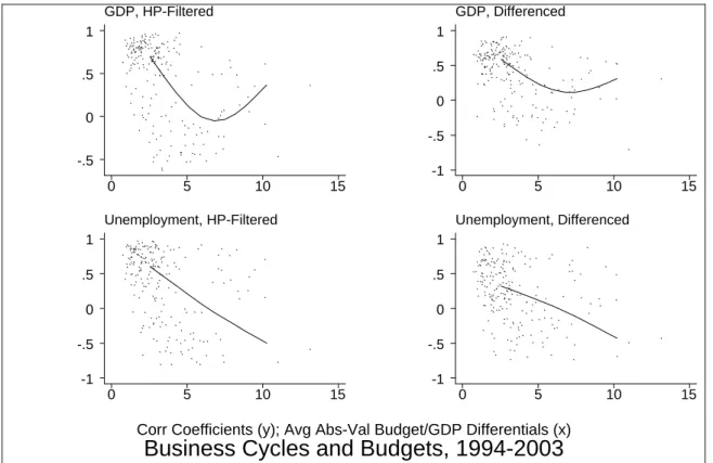
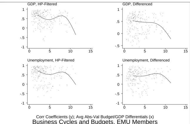
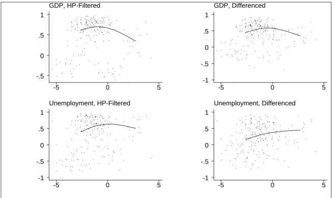
Figure 1 provides a set of four simple scatterplots of our four default measures of business cycle synchronization (GDP/Unemployment, differenced/HP-filtered) graphed against budget divergence. Non-parametric data smoothers are also provided in the graphs; these demonstrate a loose negative relationship between the two variables. Figures 2 and 3 are analogues that portray observations from the most recent (1994-2003) decade and EMU members respectively. Figure 4 is the analogue that portrays divergence in the primary (instead of the total) fiscal balance. Finally, Figures 5 and 6 are scatterplots of business cycle synchronization against the average cross-country levels of the total and primary budget positions respectively. There is reasonably consistent ocular evidence of a negative relationship between fiscal divergence and business cycle synchronization.
However, there is no sign of a strong link between the latter and the average total fiscal level, though the correlations are higher for the average primary budget position.
2.3 Estimation
Our general empirical strategy follows that of Frankel and Rose (1998) who focused on the endogeneity of business cycle synchronization with respect to trade.
The benchmark regressions we estimate are non-structural and take the simple form:
Corr(v,s)i,j,τ = α + βFiscalDivergei,j,τ + ε i,j,τ.
9 In practice there are often gaps in our data set.
Corr(v,s)i,j,τ denotes the correlation coefficient between country i and country j over decade τ for activity concept v (corresponding to log real GDP or the unemployment rate), de-trended with method s (corresponding to differencing or HP-filtering). FiscalDivergei,j,τ denotes the average (over decade τ) absolute difference in the government budget position (measured as a percentage of national GDP) between countries i and j. Finally, ε i,j,τ represents the myriad influences on bilateral activity correlations above and beyond the influences of fiscal divergence (hopefully unrelated to our regressor), and α and β are the regression coefficients to be estimated.
The object of interest to us is the slope coefficient β. A negative estimate of β indicates that an increase in fiscal divergence is associated with reduced business cycle coherence. That is, fiscal policy convergence is linked to more synchronized business cycles.
A simple OLS regression of bilateral activity income correlations on fiscal divergence might be inappropriate for a couple of reasons. First, there may be non-trivial measurement error in fiscal divergence (especially since measuring the general government budget position itself seems difficult). A potentially more important worry is simultaneity. Suppose that for some exogenous reason a high-deficit country decides to engage in long-term fiscal consolidation. If this leads to a recession, ceteris paribus, we might expect fiscal convergence to coincide with lower business cycle synchronization, at least over a short period of time.10 Alternatively, suppose that a high- deficit country decides to engage in fiscal consolidation and convergence simultaneously (e.g., during the drive to EMU); in this case, the effect goes the opposite way.
Accordingly, our default estimation is conducted with both OLS and instrumental variables.
Our instrumental variables are associated with (cross-country differences in) the size and composition of public sector activity, since the public finance/political economy literature has shown these to be of relevance (e.g., Alesina and Perotti, 1997 and Lane, 2003). Thus we use expenditure variables (such as government investment and non-wage consumption), as well as revenue variables (e.g., direct business and household taxes), all expressed as percentages of GDP.
We check that our OLS and IV results are consistent and also show that our results are insensitive to the exact choice of instrumental variables.
3. Empirics
3.1 Benchmark Results on Fiscal Convergence and Business Cycle Synchronization
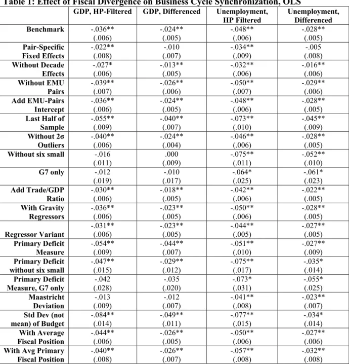
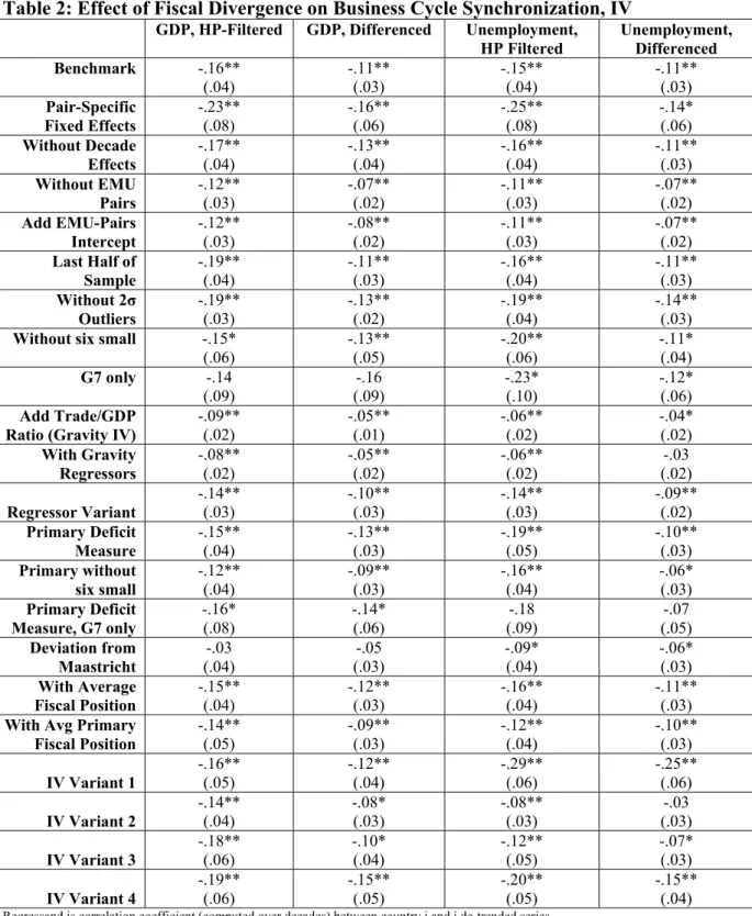
Our main results are presented in Tables 1 and 2. These display estimates of β, the estimated effect of fiscal divergence on business cycle synchronization. Robust standard errors (clustered by country-pair dyads) for the slope coefficients are presented beneath the coefficients in parentheses. One (two) asterisk(s) mark a coefficient that is significantly different from zero at the .05 (.01) confidence level. Table 1 presents OLS results, while our IV estimates are tabulated in Table 2.
The first row of each table present four benchmark estimates, one for each of our four default ways of measuring business cycle synchronization (arranged in columns). All four coefficients are negative and distinguishable from zero with a high level of statistical confidence, for both OLS and IV. Moreover, the effects are economically important. A simple average of the
10 Further, short-run fiscal spillovers results in the same problem. We try to minimize such issues by estimating our business cycle synchronizations using decades, but the issue remains.
four coefficients is -.034 for OLS. This implies that a reduction in fiscal divergence of (say) 2.5 percentage points – equal to one standard deviation in fiscal divergence – around its mean tends to raise the correlation of business cycles between a pair of countries, ceteris paribus, by around .085.
Since the average correlation coefficient in the sample is around .3, this effect is neither trivial nor implausible. The IV results are approximately four times larger, and remain highly statistically significant. We try to be conservative in estimating the magnitude of our effect (especially when the model is so simple), but are reassured by the fact that OLS and IV deliver the same sign.
Succinctly, our initial results show that fiscal convergence tends to raise business cycle synchronization.
3.2 Sensitivity Analysis
Our benchmark estimates are derived from a simple setup; before taking them seriously, it is critical to establish their robustness. The remainder of tables 1 and 2 is devoted to sensitivity analysis. In particular, we explore the robustness of our finding to: a) differences in the estimation technique; b) differences in the sample; c) the inclusion of other controls; and d) different measures of fiscal policy. None of these alters our basic finding that fiscal convergence is associated with increased business cycle synchronization.
Our analysis examines pairs of countries over different periods of time. It is thus natural to add country pair-specific (dyadic) fixed effects. When we do so, β remains negative; its statistical significance falls somewhat, while its economic importance grows substantially with IV, and shrinks with OLS. Further, the fixed effects themselves are jointly insignificant at standard levels (except for two of the OLS equations). It seems that dyadic fixed effects are not the reason for our finding of a negative β. Similarly, removing the decade (time-specific) fixed effects does not change our conclusion.
Our results seem insensitive to the exact handling of EMU observations. Dropping country- pairs that eventually joined EMU does not destroy our result; neither does adding a separate intercept for EMU dyads. Our significantly negative β estimate also survives dropping observations from the first two decades of our sample, and dropping all observations with residuals lying more than two standard deviations from zero.11
When we drop the six smallest countries from our sample (thereby halving the number of bilateral observations available to us), our results remain negative and significant when we use unemployment to measure the business cycle; the same is true when we use only G7 data.
Frankel and Rose (1998) demonstrated that trade integration had the effect of raising business cycle synchronization. Baxter-Kouparitsas (2005) showed that among the various candidates (not including our fiscal variables) suggested in the literature to determine business cycle synchronization, only trade integration has a robust effect. Might including trade in the regression reduce the effect of fiscal divergence? No. We add bilateral trade between countries i and j, normalized by the ratio of their GDPs, using four geographic determinants of the gravity model of bilateral trade as instrumental variables.12 As expected, trade has a positive and usually
11 Controlling for exchange rate volatility does not change our key result; neither does restricting the sample to countries with only limited exchange rate volatility.
12 The four instrumental variables are: 1) the natural logarithm of the great circle bilateral distance between the two countries; 2) the log of the product of the countries’ land areas; 3) a common land border dummy;
significant effect on business cycle synchronization, but its presence makes little difference to the effect of fiscal divergence on business cycles.13 Our results are also not substantially affected when we include the four gravity variables directly in our equation.14
Our next sensitivity analyses uses different variants of the fiscal divergence regressor. First, we use the absolute value of the average (over time) gap between the two countries’ budget positions, instead of using the average of the absolute value. Since budget balances are persistent, this variant delivers almost identical results to our benchmark. Second, we use (averages of absolute values of) primary budget deficits instead of total budget deficits; this delivers economically large results that remain statistically significant.15 Interestingly, these significantly negative estimates persist when we restrict our attention to either the G7 countries or the largest fifteen countries in our sample (for both GDP and unemployment). It seems that our results do not stem from any particular set of countries.
We also use the gap between the two countries’ actual government budget deficits and the Maastricht targets of a maximal 3% deficit/GDP ratio.16 Here we find weaker results; there is a statistically significant result only when we use unemployment. That is, cross-country deviations from the Maastricht convergence criteria (and thus the Stability Pact’s ceiling of 3% deficits) do not seem to have a substantial consistent effect on cycle synchronization.17
Towards the bottom of Table 1, we also use the standard deviation (computed over the ten years inside each decadal observation) of the gap between the two countries’ budget/GDP ratios, in place of our default measure of fiscal divergence. OLS estimates indicate that variation in the budget deficit positions between the countries tends to lower their business cycle synchronization, which support our benchmark results.
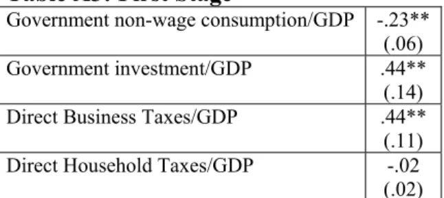
It is comforting to us that OLS and IV estimates both sign β negatively. Nevertheless, we do not have vast confidence in our instrumental variables themselves.18 (Our first stage is tabulated in Appendix Table A3; while three of the instrumental variables are significant, the R2 of the first stage is only .18.) Accordingly, we use four different sets of instrumental variables, combining measures of government revenue and expenditure series in different ways. We tabulate these results towards the bottom of Table 2. Both the economic and statistical significance of β varies depending on the estimator and measure of business cycle coherence. Still, all the estimates are negative, and the vast majority are significantly so.19
and 4) a common language dummy.
13 This is unsurprising since trade is almost uncorrelated with fiscal divergence.
14 Our results also do not change when we control for the inflation differential (an imperfect measure of monetary policy).
15 We use the OECD’s measure “Primary Government Balance, Cyclically Adjusted, % Potential GDP.”
16 We formalize this as follows. If both countries meet the 3% target, the gap between them is zero. If one meets the criterion and one has a deficit of say 4% of GDP, the gap is 1% (of GDP). If neither meets the criteria, one country’s deficit is 5% and the other’s is 6%, the difference between them is also 1% (of GDP).
17 This may be unsurprising, since there is little reason to think that convergence to 3% should have a different effect on business cycle synchronization than convergence to another deficit level.
18 For instance, we cannot exclude the possibility of simultaneity from any available fiscal aggregate.
19 We have experimented extensively with our instrumental variables, focusing especially on their cyclical sensitivity, and find that our results are robust.
We also check whether our finding (that fiscal divergence lowers business cycle synchronization) is immune to the addition of the average level of the government budget position.
That is, we add AvgFiscalto our default equation and re-estimate. As can be seen from the bottoms of Tables 1 and 2, the effect of fiscal divergence on business cycle synchronization is unaffected when we control for the level of the average (cross-country) fiscal deficit; β remains economically and statistically significant.
3.3 Further Robustness Checks
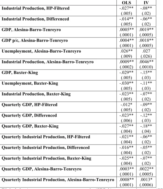
Table 3 provides more sensitivity checks, using a number of different measures of business cycle synchronization. Rather than rely on a single measure of business cycle coherence in the benchmark results, we used four measures in Tables 1 and 2. Still, there is no reason not to try others. The rows of Table 3 correspond to the estimated effect of fiscal divergence on fifteen further measures of business cycle synchronization. In different columns we provide OLS and IV estimates of β.
The first rows of Table 3 use industrial production (rather than GDP or unemployment) as the underlying measure of economic activity. Next, we follow Alesina, Barro and Tenreyro (2002) in measuring business cycle divergence. Alesina et al first construct the ratio of the two countries’
log real GDP; they then regress that ratio on two of its lags and an intercept. The root mean squared error of the residual is their measure of business cycle divergence. Since a smaller number implies greater synchronization, we expect the sign of β to be reversed (compared with that of the correlation coefficient of de-trended business cycles). We construct Alesina-Barro-Tenreyro measures for log real GDP, log real GDP per capita, the unemployment rate, and the log of industrial production.
A third set of checks uses the Baxter-King (1999) band-pass filter to de-trend the underlying data (we use 2-8 years, corresponding to their 6-32 quarters). Finally, we switch to using underlying quarterly data rather than annual data. The finer frequency comes at a cost of a smaller data span.
None of the results in Table 3 alter our conclusions. The checks work well in the sense that β remains significantly negative for almost all the perturbations.20
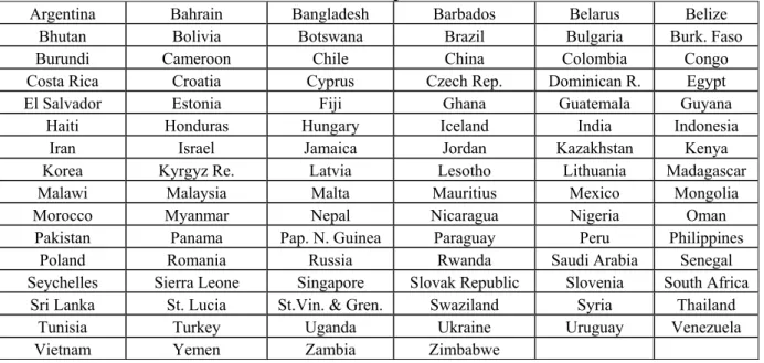
As an additional robustness check, we broadened the country coverage to include developing countries as well. This extended database covers 115 countries (hence it has a maximum of 6555 [=115*114/2] bilateral country-pairs) for four decades. Since the unemployment rate and our instrumental variables are missing for many observations, we are constrained to use only GDP and OLS. The results are tabulated in Table A6. As in Tables 1 and 2, we find a negative and mostly significant relationship between fiscal divergence and business cycle synchronization (though when pair-specific effects are included, the coefficients lose significance).
3.4 Does the Average Budget Position have an Effect on Business Cycle Synchronization?
Thus far we have found strong evidence that persistent cross-country differences in government budget positions have a (negative) effect on the synchronization of their business cycles. An interesting but different question is whether the average (cross-country) levels of
20 We have also used 20- and 40-year periods instead of decades, and our key results remain.
government budget positions also affect business cycle synchronization. We now investigate that issue.21
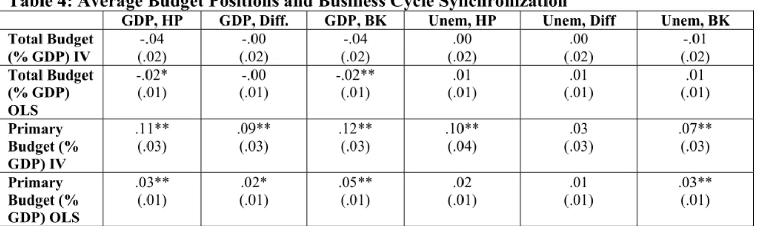
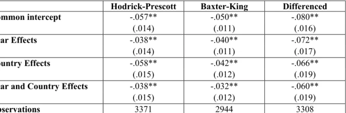
Table 4 contains estimates of the effect of the average (across pair of countries) government budget position on business cycle synchronization. Since we analyze two underlying concepts of economic activity (GDP and unemployment), three de-trending techniques (HP-filtering, differencing, and BK-filtered), two estimators (OLS and IV), and two budget concepts (total and primary), we provide twenty-four (=2*3*2*2) different point estimates and their standard errors.
We find little evidence that the total budget deficit has a consistent effect on business cycle synchronization. Seven of the twelve estimates are negative (two of those are statistically significant), while five are positive (non significant). All are small. However, all twelve of the coefficients for the primary budget effects are positive, three-quarters of them significantly so. We interpret the evidence as indicating that lower primary fiscal deficits (or higher primary surpluses) enhance business cycle synchronization. Further, when we use our extended sample of 115 countries, the average total budget balance has a positive and significant effect on synchronization, as can be seen from the last column of Table A6.
Still, we do not wish to over-interpret our findings. The average primary budget position is negatively correlated with our default measure of fiscal divergence (as can be seen from Table A2).
When we include both fiscal divergence and the average primary budget position in our regressions, the former remains significantly negative (as can be seen from Tables 1 and 2), while the latter effect loses the horse-race (its effect becomes economically and statistically small, and varies across specifications). We have searched without success for a non-linear or interactive effect, and consider this to be a good topic for future research. That is, there is evidence that primary fiscal consolidation enhances business cycle synchronization, but it is weak. By way of comparison, there is strong evidence that fiscal divergence (of both total and primary balances) reduces the coherence of business cycles.22
4. Interpretation: Fiscal Irresponsibility tends to be Idiosyncratic
In section 3, we established that fiscal convergence seems to induce greater business cycle synchronization. If one takes the finding as given, the question remains: Why? We think the answer is that fiscal divergence tends to occur when one country runs a substantially and persistently higher budget deficit than other countries, and simultaneously creates fiscal shocks.
That is, irresponsible fiscal policy (a persistently high deficit) coincides with idiosyncratic (fiscal) instability. When the budget deficit is closed (fiscal convergence), the fiscal shocks diminish;
business cycles tend to become more synchronized. Succinctly, fiscal policy that is irresponsible is
21 We have already shown in Tables 1 and 2 that controlling for the average level of the government budget position (i.e., including AvgFiscal in our regressions) has little effect on the economic or statistical significance of β.
22 We have also briefly investigated the effects of other Maastricht criteria on business cycle synchronization; estimates appear in Table A5. There is some evidence that exchange rate volatility, and divergence in inflation, long interest rates, and government debt levels all tend to lower business cycle synchronization. However, none of the effects is particularly strong or consistent. We view this as an area worthy of future research.
also fiscal policy that creates idiosyncratic shocks and thus macroeconomic volatility. This idea is both intuitive and consistent with the literature (e.g., Fatás and Mihov, 2003a, 2004).
4.1 Direct Evidence on Budgets and Macroeconomic Volatility via a Unilateral Panel
We now test our intuition in a straightforward way. We are interested in testing for a (negative) link between a country’s average budget position and its business cycle volatility. Our evidence thus far has relied on bilateral data, comparing fiscal policy of pairs of countries to the synchronization of their business cycles. It is also possible to check this idea more directly using a unilateral (though still non-structural) approach. Accordingly, we gather a panel of annual data for 115 countries (see Appendix Table A1b) between 1960 and 2003 (with gaps), consisting of data on real GDP and the total government budget position (as a percentage of GDP; surpluses are positive, deficits negative).23 We then de-trend the output data by differencing and using both the HP and BK filters to create measures of business cycle fluctuations. We compare both the average absolute value of these business cycle deviations, and their volatility – proxied by the standard deviation (estimated for a country over time) – to the average level of the government’s fiscal position. A negative relationship between the two indicates that smaller deficits or larger surpluses are associated with reduced business cycle volatility, consistent with our hypothesis.
We exploit our (country x year) panel of data in three different ways. First, we estimate panel regressions of the effect of the government budget position on business cycle deviations from trend at the annual frequency. Second, we split our 44-year data set into four eleven-year periods, so that each country contributes a maximum of four observations. Finally, we average over all 44 years, creating a single cross-section where each country contributes a single observation. For the first two cases, we estimate our models with differing sets of country- and time-specific fixed effects.
Our results are contained in Table 5. The top panel portrays annual results; the middle presents results estimated at the 11-year frequency; and the bottom shows cross-sectional results that average out the entire 44-year sample.
The point estimates from our annual results are all negative; a higher fiscal surplus (or lower deficit) is associated with smaller (in absolute value) business cycle deviations from trend. The results are statistically significant at conventional levels for twelve perturbations. When we shift to a lower frequency, we can examine both the average (over eleven years) of the mean absolute value of business cycle deviations, and the volatility of business cycles (the standard deviation of de- trended log real GDP). 20 of the 24 point estimates are negative, eight significantly so; none of the positive coefficients is economically or statistically large. Finally, when we examine a single cross-section of our countries, we again find that larger fiscal surpluses/smaller deficits are associated with lower business cycle volatility. At this very low frequency, all six point estimates are negative and half of them are significantly different from zero at standard confidence levels.
We do not consider this evidence to be overwhelming. Since we have essentially no structure in our empirical model, our results are suggestive rather than definitive. Still, we have not found evidence inconsistent with our hypothesis either in the literature or in our own empirical
23 We do not know of a source that systematically provides primary fiscal positions for countries outside the OECD.
work. The hypothesis that larger fiscal deficits tend to be associated with greater business cycle volatility seems reasonable and awaits further scrutiny.
5. Conclusion
The motivation for this paper is simple. The criteria that make a currency area optimal were established long ago by Mundell and have essentially no intersection with the “Maastricht convergence” criteria used to govern the actual entry of countries into European Monetary Union.
In this paper, we ask: does Maastricht indirectly overlap with Mundell?
The answer is positive. We find that fiscal convergence – similarity in the aggregate budget positions across countries – is systematically associated with enhanced business cycle synchronization. Fiscal convergence raises business cycle synchronization by eliminating idiosyncratic fiscal shocks. We find evidence that reduced primary fiscal deficits (or higher surpluses) also increase the coherence of business cycles across countries. The Maastricht convergence process encouraged both fiscal convergence and reduced deficits for the Euro-12 during the run-up to EMU. Our results indicate that this fiscal convergence would have raised their business cycle coherence, making them better candidates for currency union. Even if not by design, Maastricht mimics Mundell!
There is a different (though consistent) interpretation of our results. Conventional wisdom tells us that national fiscal policy is the sole macroeconomic tool to smooth the business cycle when a country is hit by asymmetric shocks in a currency union. Yet the Maastricht criteria impose convergence of budget deficits at low levels. Consequently, Maastricht could reduce business cycle synchronization and increase volatility. In fact though, fiscal convergence seems to increase cycle synchronization by reducing volatile fiscal shocks.
If our finding is corroborated, it is of more than academic interest. The Maastricht criteria continue to govern future entry into the euro zone. Further, the Stability and Growth Pact continues, in principle, to constrain fiscal policy for the EU. If either or both of these institutions induce fiscal convergence, they indirectly enhance the desirability and sustainability of EMU. Two cheers!
Table 1: Effect of Fiscal Divergence on Business Cycle Synchronization, OLS
GDP, HP-Filtered GDP, Differenced Unemployment, HP Filtered
Unemployment, Differenced Benchmark -.036**
(.006)
-.024**
(.005)
-.048**
(.006)
-.028**
(.005) Pair-Specific
Fixed Effects -.022**
(.008) -.010
(.007) -.034**
(.009) -.005
(.008) Without Decade
Effects -.027*
(.006) -.013**
(.005) -.032**
(.006) -.016**
(.006) Without EMU
Pairs
-.039**
(.007) -.026**
(.006) -.050**
(.007) -.029**
(.006) Add EMU-Pairs
Intercept
-.036**
(.006)
-.024**
(.005)
-.048**
(.006)
-.028**
(.005) Last Half of
Sample -.055**
(.009) -.040**
(.007) -.073**
(.010) -.045**
(.009) Without 2σ
Outliers -.040**
(.006) -.024**
(.004) -.046**
(.006) -.028**
(.005) Without six small -.016
(.011) .000
(.009) -.075**
(.011) -.052**
(.010) G7 only -.012
(.019)
-.010 (.017)
-.064*
(.025)
-.061*
(.023) Add Trade/GDP
Ratio -.030**
(.006) -.018**
(.005) -.042**
(.006) -.022**
(.005) With Gravity
Regressors -.036**
(.006) -.023**
(.005) -.050**
(.006) -.028**
(.005) Regressor Variant
-.031**
(.006) -.023**
(.005) -.044**
(.005) -.027**
(.005) Primary Deficit
Measure
-.054**
(.009)
-.044**
(.007)
-.051**
(.010)
-.027**
(.009) Primary Deficit
without six small -.047**
(.015) -.029**
(.012) -.075**
(.017) -.035*
(.014) Primary Deficit
Measure, G7 only -.042
(.028) -.035
(.020) -.073*
(.031) -.055*
(.025) Maastricht
Deviation
-.013
(.009) -.012
(.007) -.041**
(.008) -.023**
(.007) Std Dev (not
mean) of Budget
-.084**
(.014)
-.049**
(.011)
-.077**
(.015)
-.034*
(.014) With Average
Fiscal Position -.044**
(.006) -.026**
(.005) -.050**
(.006) -.027**
(.006) With Avg Primary
Fiscal Position -.040**
(.008) -.026**
(.007) -.057**
(.008) -.032**
(.008)
Regressand is correlation coefficient (computed over decades) between country i and j de-trended series.
Coefficients recorded are effect of (average of absolute-value of differential of) government budget surplus/deficit, as percentage of GDP. Robust standard errors (clustered by country-pair dyads) recorded in parentheses. Decade effects and constant included but not recorded.
Coefficients significantly different from zero at .05 (.01) level marked with one (two) asterisk(s). OLS estimation unless noted.
Data set has maximum of 21*20/2=210 country pairs for four decades (1964-73, 1974-83, 1984-93, 1994-2003).
Six small countries: Denmark, Finland, Greece, Ireland, Norway, and New Zealand.
Regressor variant is absolute value of average of differential (not average of absolute-value of differential). Std Dev is standard deviation over time of absolute value of differential of government budget surplus/deficit, % GDP.
Table 2: Effect of Fiscal Divergence on Business Cycle Synchronization, IV
GDP, HP-Filtered GDP, Differenced Unemployment, HP Filtered
Unemployment, Differenced Benchmark -.16**
(.04)
-.11**
(.03)
-.15**
(.04)
-.11**
(.03) Pair-Specific
Fixed Effects -.23**
(.08) -.16**
(.06) -.25**
(.08) -.14*
(.06) Without Decade
Effects -.17**
(.04) -.13**
(.04) -.16**
(.04) -.11**
(.03) Without EMU
Pairs
-.12**
(.03) -.07**
(.02) -.11**
(.03) -.07**
(.02) Add EMU-Pairs
Intercept
-.12**
(.03)
-.08**
(.02)
-.11**
(.03)
-.07**
(.02) Last Half of
Sample -.19**
(.04) -.11**
(.03) -.16**
(.04) -.11**
(.03) Without 2σ
Outliers -.19**
(.03) -.13**
(.02) -.19**
(.04) -.14**
(.03) Without six small -.15*
(.06) -.13**
(.05) -.20**
(.06) -.11*
(.04) G7 only -.14
(.09)
-.16 (.09)
-.23*
(.10)
-.12*
(.06) Add Trade/GDP
Ratio (Gravity IV) -.09**
(.02) -.05**
(.01) -.06**
(.02) -.04*
(.02) With Gravity
Regressors -.08**
(.02) -.05**
(.02) -.06**
(.02) -.03
(.02) Regressor Variant
-.14**
(.03) -.10**
(.03) -.14**
(.03) -.09**
(.02) Primary Deficit
Measure
-.15**
(.04)
-.13**
(.03)
-.19**
(.05)
-.10**
(.03) Primary without
six small -.12**
(.04) -.09**
(.03) -.16**
(.04) -.06*
(.03) Primary Deficit
Measure, G7 only -.16*
(.08) -.14*
(.06) -.18
(.09) -.07
(.05) Deviation from
Maastricht
-.03
(.04) -.05
(.03) -.09*
(.04) -.06*
(.03) With Average
Fiscal Position
-.15**
(.04)
-.12**
(.03)
-.16**
(.04)
-.11**
(.03) With Avg Primary
Fiscal Position -.14**
(.05) -.09**
(.03) -.12**
(.04) -.10**
(.03) IV Variant 1 -.16**
(.05) -.12**
(.04) -.29**
(.06) -.25**
(.06) IV Variant 2
-.14**
(.04) -.08*
(.03) -.08**
(.03) -.03
(.03) IV Variant 3
-.18**
(.06)
-.10*
(.04)
-.12**
(.05)
-.07*
(.03) IV Variant 4 -.19**
(.06) -.15**
(.05) -.20**
(.05) -.15**
(.04)
Regressand is correlation coefficient (computed over decades) between country i and j de-trended series.
Coefficients recorded are effect of (average of absolute-value of differential of) government budget surplus/deficit, as percentage of GDP. Robust standard errors (clustered by country-pair dyads) recorded in parentheses. Decade effects and constant included but not recorded.
Coefficients significantly different from zero at .05 (.01) level marked with one (two) asterisk(s).
Instrumental Variable estimation unless noted. IVs include: a) government non-wage consumption/GDP; b) government investment/GDP; c) direct business taxes/GDP; and d) direct household taxes/GDP. IVs are average of absolute value of cross-country differentials.
Data set has maximum of 21*20/2=210 country pairs for four decades (1964-73, 1974-83, 1984-93, 1994-2003). Six small countries: Denmark, Finland, Greece, Ireland, Norway, and New Zealand.
Regressor variant is absolute value of average of differential (not average of absolute-value of differential). Std Dev is standard deviation over time of absolute value of differential of government budget surplus/deficit, % GDP.
IV Variant 1: a) government non-wage consumption/GDP; b) government investment/GDP; c) effective labor taxes as percentage of labor costs; and d) indirect taxes/GDP. Variant 2: a) government social benefits/GDP: b) government wages/GDP; and c) direct business taxes/GDP. Variant 3: a) direct household taxes/GDP; b) indirect taxes/GDP; and c) direct business taxes/GDP. Variant 4: a) government non-wage consumption/GDP; b) government wages/GDP; and c) government investment/GDP.
Gravity regressors are: 1) log distance; 2) log product land area; 3) common land border dummy; 4) common language dummy.
Table 3: Fiscal Divergence and Different Measures of Business Cycle Synchronization
OLS IV
Industrial Production, HP-Filtered -.027**
(.005) -.08**
(.02) Industrial Production, Differenced -.014**
(.005)
-.06**
(.02)
GDP, Alesina-Barro-Tenreyro .0005**
(.0001) .0019**
(.0005) GDP p/c, Alesina-Barro-Tenreyro .0004**
(.0001) .0018**
(.0005) Unemployment, Alesina-Barro-Tenreyro .026**
(.009) .027 (.026) Industrial Production, Alesina-Barro-Tenreyro .0009**
(.0002)
.0046**
(.0010)
GDP, Baxter-King -.029**
(.005) -.15**
(.03)
Unemployment, Baxter-King -.030**
(.005) -.11**
(.03) Industrial Production, Baxter-King -.023**
(.005) -.07**
(.02)
Quarterly GDP, HP-Filtered -.012*
(.005)
-.09**
(.02)
Quarterly GDP, Differenced -.023**
(.006) -.12**
(.03)
Quarterly GDP, Baxter-King -.027**
(.004) -.18**
(.04) Quarterly Industrial Production, HP-Filtered -.021**
(.004) -.06**
(.02) Quarterly Industrial Production, Differenced -.016**
(.004)
-.05**
(.02) Quarterly Industrial Production, Baxter-King -.025**
(.004) -.07**
(.02) Quarterly GDP, Alesina-Barro-Tenreyro .0003**
(.0001) .0022**
(.0005) Quarterly Industrial Production, Alesina-Barro-Tenreyro .0008**
(.0001) .0013*
(.0006)
IVs include: a) government non-wage consumption/GDP; b) government investment/GDP; c) direct business taxes/GDP; and d) direct household taxes/GDP. IVs are average of absolute value of cross-country differentials.
Coefficients recorded are effect of (average of absolute-value of differential of) government budget surplus/deficit, as percentage of GDP.
Coefficients significantly different from zero at .05 (.01) level marked with one (two) asterisk(s)
Data set has maximum of 21*20/2=210 country pairs for four decades (1964-73, 1974-83, 1984-93, 1994-2003).
Decade effects and constant included but not recorded.
Alesina-Barro-Tenreyro measure is root mean squared error of residual from AR(2) of log ratios (lower => greater co- movement).
Robust standard errors (clustered by country-pair dyads) recorded in parentheses.
Table 4: Average Budget Positions and Business Cycle Synchronization
GDP, HP GDP, Diff. GDP, BK Unem, HP Unem, Diff Unem, BK Total Budget
(% GDP) IV
-.04
(.02) -.00
(.02) -.04
(.02) .00
(.02) .00
(.02) -.01
(.02) Total Budget
(% GDP) OLS
-.02*
(.01)
-.00 (.01)
-.02**
(.01)
.01 (.01)
.01 (.01)
.01 (.01) Primary
Budget (%
GDP) IV
.11**
(.03) .09**
(.03) .12**
(.03) .10**
(.04) .03
(.03) .07**
(.03) Primary
Budget (%
GDP) OLS
.03**
(.01)
.02*
(.01)
.05**
(.01)
.02 (.01)
.01 (.01)
.03**
(.01) IVs include: a) government non-wage consumption/GDP; b) government investment/GDP; c) direct business taxes/GDP; and d) direct household taxes/GDP. IVs are average of absolute value of cross-country differentials.
Coefficients recorded are effect of cross-country average level of total/primary government budget surplus/deficit, as percentage of GDP.
Coefficients significantly different from zero at .05 (.01) level marked with one (two) asterisk(s)
Data set has maximum of 21*20/2=210 country pairs for four decades (1964-73, 1974-83, 1984-93, 1994-2003).
Decade effects and constant included but not recorded.
Robust standard errors (clustered by country-pair dyads) recorded in parentheses.