A New Method For Combining Detrending Techniques with Application to Business Cycle Synchronization of the New EU Members

CORVINUS UNIVERSITY OF BUDAPEST

DEPARTMENT OF MATHEMATICAL ECONOMICS AND ECONOMIC ANALYSIS Fővám tér 8., 1093 Budapest, Hungary Phone: (+36-1) 482-5541, 482-5155 Fax: (+36-1) 482-5029 Email: zsolt.darvas@uni-corvinus.hu

W ORKING P APER

2005 / 5

A N EW M ETHOD F OR C OMBINING D ETRENDING

T ECHNIQUES WITH A PPLICATION TO B USINESS C YCLE

S YNCHRONIZATION OF THE N EW EU M EMBERS

Zsolt Darvas and Gábor Vadas

Budapest, 2005.

A New Method for Combining Detrending Techniques with Application to Business Cycle Synchronization of the New EU Members

^♦

Zsolt Darvas and Gábor Vadas

Draft Revised as of: August 15, 2005

Abstract

Decomposing output into trend and cyclical components is an uncertain exercise and depends on the method applied. It is an especially dubious task for countries undergoing large structural changes, such as transition countries. Despite their deficiencies, however, univariate detrending methods are frequently adopted for both policy oriented and academic research. This paper proposes a new procedure for combining univariate detrending techniques which is based on revisions of the estimated output gaps adjusted by the variance of and the correlation among output gaps. The procedure is applied to the study of the similarity of business cycles between the euro area and new EU Member States.

JEL Classification: C22, E32

Keywords: combination, detrending, new EU members, OCA, output gap, revision

♦ Darvas is Assistant Professor, Department of Mathematical Economics and Economic Analysis, Corvinus University Budapest. He was affiliated with the Magyar Nemzeti Bank throughout most of the research process. E-mail: zsolt.darvas@uni-corvinus.hu Vadas is Senior Economist, Economics Department, Magyar Nemzeti Bank. E-mail: vadasg@mnb.hu

We wish to thank Fabio Canova, Wojciech Charemza, Lavan Mahadeva, András Simon, Balázs Vonnák, conference participants at the ECOMOD2005, and seminar participants at the ADATEF, Eötvös Lóránd University and Magyar Nemzeti Bank for helpful comments and suggestions. The views expressed are those of the authors and do not necessarily reflect the official views of the Magyar Nemzeti Bank. The dataset and an EViews program that reproduces our results are available at www.uni-corvinus.hu/darvas.

1.

Introduction

The potential or permanent component of output is an important unobserved variable for decision making, policy analysis, and macroeconomic modeling. For instance, sustainability of fiscal positions and monetary policy actions is frequently evaluated in the light of the cyclical position of an economy. Another example is the study of business cycle correlation for an optimum currency area analysis.

Estimating potential output, though, is very difficult even in the case of developed countries.

Deficiencies are not mainly associated with the complexities of empirical methods, but rather with the mapping of an economic concept of potential output into a plotted time series. There are dozens of methods and models for empirical estimation: some are intended to measure potential output and the output gap, others call their objectives trends and cycles, while terms permanent and transitory components are also frequently used. The common idea behind these methods is to reveal a component which is likely to persist over the long-run.¹ Critiques stemming from properties and economic implications characterize all methods. Those who employ multivariate methods criticize univariate models on the grounds that such methods do not take into account all relevant information. Those who prefer non-structural methods (either univariate or multivariate) criticize structural multivariate approaches by applying a priori structures to the economy which may be invalid. Univariate modelers usually favor their methods because of simplicity and the absence of a number of ad hoc assumptions; several univariate methods, however, make one very important ad hoc assumption.

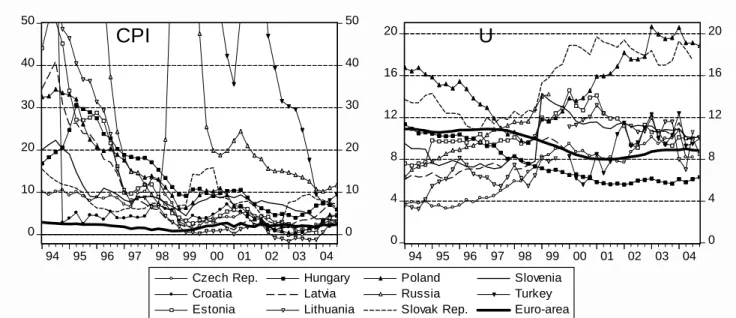
Disagreement on the mapping of the concept into empirical estimates in mature economies renders estimates even more problematic for countries facing deep structural changes, such as transition economies. Although most transition countries had already introduced some market institutions by the end of the 1980s, processes such as democratization, further decentralization, the collapse of COMECON, privatization, comprehensive adoption of market institutions, market opening and Western integration exposed these economies to dramatic changes. As a natural consequence, standard models might not work for the transition period lasting several years. For example, the considerable downturn in the early years of transition was accompanied by a massive rise in inflation, while inflation contracted during periods of rapid growth in several countries (Figure 1). Issues of structural changes and non-applicability of standard concepts are coupled with poor quality and short databases. Emergence of thousands of enterprises and retail stores, quickly changing product and quality structures, posed huge challenges to statistical offices. Many important figures are simply not available for several years back and the available data necessary for potential output estimates are mostly at annual frequency. Quarterly national accounts figures started to be published only in the second half of the nineties and were frequently subject to major

1Throughout this paper the terms potential output/trend output/permanent component of output and output gap/cycle/transitory component are regarded as synonymous. Although there is a slight difference among the generally assumed ideas behind these concepts, the same methods were applied to recover all of them. Policy makers and global agencies use the terms potential output and output gap more frequently, while academics mostly prefer the former expressions.

revisions. The aforementioned drawbacks leave us very cautious when it comes to estimating potential output figures for transition economies.

Despite conceptual and practical concerns, the need for output gap measures led almost all central banks of the new EU Member States and dozens of academic researchers to estimate some measures using various univariate detrending techniques. A remedy for these applications is provided by Smets-Wouters (2003), who tried to answer the question of why central banks use various filters if modern New-Keynesian micro-founded models predict that the appropriate target level of output, which usually corresponds to flexible-price level of output, may be more volatile than actual output. Their answer is that not every shock should affect the target level of output, on the one hand, and in practice it is difficult to decide the nature of shocks, on the other. Under such circumstances the target level of output could be smooth.

One of the most frequently studied issues with the help of estimated output gap figures was business cycle correlation with the euro area, motivated by optimum currency area considerations.

Fidrmuc-Korhonen (2004), for instance, surveyed 31 papers studying this issue. In this paper we adopt various univariate techniques for calculating the cyclical component of GDP and study the dependency of the cyclical correlation with the euro area on the method selected, for quarterly GDP data in 1993Q1-2004Q4. Hence, our primary goal is similar to Canova (1998), who compared the results of ten filters on business cycle properties. Our results will also be similar since we will also document the dependency of results on methods. This raises the question whether there is any use of adopting these filters, as all of them have conceptual weaknesses and none of them can be selected as ‘the best’. However, the need for filters is rather strong from the perspective of both economic policy and academic research. Therefore, we propose a new procedure that is able to combine various techniques into a single measure. As standard errors, which might be used for deriving weights, are not available for some of the methods, we base our weights on similar but computable statistics, namely on revisions of the output gap for all dates by recursively estimating the models. We will compare our combining procedure to the most widely used one, to the principal components analysis. Findings indicate that the results of our procedure do not differ much from the results achieved by principal component analysis, but our procedure has in many cases much smaller revisions and never derives negative weights, therefore, we regard it preferable.

The rest of paper is structured as follows. Section 2 reviews the concepts of potential output and underlines its limitations for open economies in general and for transition economies in particular. Section 3 introduces and discusses the univariate filtering methods we use and describes our procedure of combining methods. Section 4 describes the data, Section 5 presents the results, and Section 6 concludes.

2.

Concepts of potential output

2.1. Mainstream concepts

Probably the most widely adopted concept of potential output is the level of output that represents a balanced state of the economy. This balanced state is frequently defined as stable inflation. Stable inflation corresponding to a certain level of unemployment is called NAIRU (non-accelerating inflation rate of unemployment) which relates to a certain level of output via the Okun-law.

However, NAIRU is not easy to measure because of structural and hysteresis reasons. Partly due to

this reason and partly due to theoretical Phillips-curve considerations, there are models that use inflation directly as information about the output gap.²

The so-called production function method analyses factor inputs to production. It is usually combined with the concept of NAIRU; thus the potential labor input is taken into account instead of the actual labor input.³

Another line of the literature defines potential output as the level of output free of the effect of demand shocks. Demand and supply shocks are frequently studied in the framework of SVARs pioneered by Blanchard–Quah (1989). They estimated a two-variable VAR model for output and unemployment and constrained the parameters the following way. There are two types of shocks:

(1) supply shocks have a transitory effect on unemployment and a permanent effect on output; (2) demand shocks have a transitory effect on both variables. Behind these constraints there is a model in which the permanent shocks can be interpreted as supply shocks and the transitory shocks as demand shocks.⁴

A further class of models assumes that potential output is driven by exogenous productivity shocks that determine long-run growth. Short-run developments in output are due to the behavior of rational agents who react to unexpected productivity shocks by writing off old capacities and rearranging resources to new conditions.

We argue that, in addition to the highlighted conceptual weaknesses of NAIRU and the econometric weaknesses of the SVARs,⁵ the assumptions behind these models are rather questionable for open economies in general and for transition countries in particular.

2.2. The transition shock

We argue that standard concepts are incapable of describing transition shocks.

In the period of transition the economy was shocked by enormous relative price changes,⁶ which resulted in a structural change in demand. The structure of supply was unable to adjust to this change quickly. Therefore, capacities became redundant while new capacities were established only in a gradual evolutionary process. Meanwhile, excess demand and excess supply existed side by side, and aggregate output decreased because the short-side rule prevailed in each micro market.

The decline in output brought about unemployment.

It is rather difficult to assign the nature of this shock either to supply or demand. The definition based on the concept of demand as aggregate planned purchases and supply as aggregate planned

2 See, e.g. Kuttner (1994) and Gerlach–Smets (1999).

3 See Giorno et al. (1995) and Denis–McMorrow–Werner (2001). As described in Giorno et al. (1995), the OECD Secretariat used the split time trends (= segmented deterministic trends) method with ad hoc judgements up to the first half or the 1980s, then switched to the production function (PF) approach.

4 The data induced even Blanchard-Quah (1989) to adopt an atheoretical pre-filter: they detrended the unemployment rate with a broken deterministic trend.

5 See, for instance, Faust and Leeper (1997), Cooley and Dwyer (1998) and their references.

6 Due to the transfer to a system of market pricing.

sales does not help much in finding the answer, as it was the structure and not the aggregate amount that differed.

The definition of aggregate excess demand implies that a demand shock would create excess demand in the short run, but does not affect output in the long run. A supply shock related mostly to technical changes would have permanent effects. Generally, supply shocks may have transitory effects as well. A monetary squeeze affects both supply and demand temporarily, as supply is constrained through the credit channel. Similarly, a structural shock may have transitory effects.

This has led to the reinterpretation of demand and supply shocks: in several contexts they do not mean changes in planned purchases or planned sales, but only the temporary or permanent nature of the shock.⁷ The question may arise whether the recession of the early 1990s in transition economies was the result of a temporary or a permanent negative shock. On the one hand, the high rate of unemployment that has arisen would suggest that the shock was temporary. On the other hand, it is clear that the persistence of the crisis is longer than the persistence of the usual excess-demand driven business cycle recessions. If output drops below its equilibrium level because of the lack of aggregate demand, then it is the speed of price adjustment that determines the length of the impact of the shock. However, if output drops because of a structural mismatch, not only prices have to adjust, but the structure of supply as well. This is presumably much slower than price adjustment, because it requires the establishment of whole new production cultures. The inertia in this process is too large to be explained by pure construction costs: uncertainties owing to limited information constrain the speed of adjustment decisively.⁸

How long does the effect of a transitory shock last? In practice in finite samples it is difficult to separate shocks which have an autoregressive representation with dominant (inverted) roots that are 1 from those which have roots less than 1. Sometimes it is useful to consider some roots to be 1 even though theory would tell that they are less than 1. In this manner, some shocks that are transitory in theory may be considered as permanent in some models. Although it is true that employment reverts to its natural rate and therefore its fluctuation introduces a transitory element into output, the observation period of the transition countries did not render either the quality or the variability of data that would be required for using them as information on this effect. Therefore, in Hungary for example, even though unemployment rose from 0 to 13 percent after the system change in 1990 and then slowly declined to 6 percent (Figure 1), we do not consider the slow decline of unemployment as an important element of a transitory increase in output.

The persistence of unemployment as a result of this structural shock is similar to the phenomenon of hysteresis. The difference is that in the literature on hysteresis the emphasis is on the fact that unemployment erodes the capabilities of the worker, while in the case of a structural shock it is the production environment (structure of capacity, geographic location, and invisible business capital) that erodes and cannot be recovered.

7 For example, the univariate trend-cycle decompositions that we study adopt this interpretation.

8 See Stiglitz (1992) for a thorough development of this argument.

2.3. Open economy considerations

Renouncing unemployment as a source of information may be motivated from another aspect as well. We do not even use information given by inflation data, as the steady fall in inflation in the second half of the 1990s (Figure 1) should not be regarded as the result of a continuously negative output gap. Rather, it may have been the consequence of the larger weight of expectations than inertia in a standard neo-Keynesian Phillips-curve.⁹

However, in an open economy excess demand may simply result in increased imports without any direct effect on inflation. Increased imports may have an impact on future inflation, but the effects may be variable both in lags and magnitude, depending on policies and on whimsical business sentiment. In addition, during our sample period inflation was still hit by shocks related to the transition process,¹⁰ so one could face insurmountable difficulties when trying to decompose these shocks.¹¹

3.

Empirical methods

In the previous section we argued that standard structural methods for output gap calculations are not applicable for open economies in general and for transition countries in particular. Therefore, we study univariate filters and the post-transition sample starting in 1993. Obviously, a general weakness of univariate methods is their very nature of being univariate: they take into consideration neither the consequences of non-zero output gaps, nor structural constraints and limitations of growth. However, the results of Smets-Wouters (2003) indicate that even from a New-Keynesian SDGE perspective the use of univariate filtering could be justified.

There are some surveys available on potential output/trend/permanent component measurement. The most wide-ranging survey can be found in Canova (1998), who compares the properties of the cyclical components of US data using seven univariate (Hodrick–Prescott filter, Beveridge–Nelson decomposition, linear trend, segmented trend, first order differencing, unobservable components model, frequency domain masking) and three multivariate (cointegration, common linear trend and multivariate frequency domain) detrending techniques. His conclusion is that, both quantitatively and qualitatively, properties of business cycles vary widely across detrending methods and that alternative detrending filters extract different types of information from the data.

A similar conclusion was reached by some other papers comparing fewer methods. For example, Dupasquier–Guay–St-Amant (1997) focus on three multivariate methodologies: structural vector autoregression, multivariate Beveridge–Nelson decomposition, and Cochrane’s methodology, and compare the results to some univariate filters. They arrive at the conclusion that

9 It is well known that under certain parameter values, including a large weight of expectations in the new keynesian Phillips-cure, disinflation can be costless in small macromodels (see Benczúr-Simon-Várpalotai, 2002).

10 For example, hardly quantifiable expectations in the circumstances of a highly uncertain system change, substantial price liberalization, and administered price rises.

11 For example, Darvas–Simon (2000) developed a model which makes use of the information that is rendered by the openness of the economy.

statistical properties of cycles derived from different methods are dissimilar, conclusions regarding certain recessions in the US are different, and also highlight that the confidence intervals of different measures are generally wide. Harvey–Jaeger (1993) compare some univariate models: the structural time series models of Harvey (1989), the Hodrick–Prescott filter, Beveridge–Nelson decomposition, and the segmented trend approach. They argue that all but the structural times series models suffer from significant deficiencies and make a case for their so called ‘structural models’, which are univariate unobserved-components techniques. Stock-Watson (1999) study the Hodrick- Prescott and Band-Pass filter, and argue that the BP filter is preferable from a theoretical point of view, but the BP filter also has weaknesses, since in finite samples only various approximations could be used.

The Beveridge–Nelson decomposition assumes that potential output follows a random walk.

Lippi–Reichlin (1994) and Dupasquier–Guay–St-Amant (1997) criticize this assumption arguing that the random walk model of potential output is inconsistent with the generally accepted view of productivity growth. They argue that technology shocks are likely to be absorbed gradually by the economy because of adjustment costs, learning, and the time-consuming process of investments, for example.

Still, perhaps the most commonly applied filter is the HP filter. Cogley–Nason (1995) directly studied the properties of this filter. They showed that when applied to stationary time series (including trend-eliminated trend-stationary series), the HP filter works as a high-pass filter, that is, suppresses cycles with higher frequencies while letting low frequency cycles pass through unchanged. However, for different stationary series, the HP filter is not a high-pass filter, but suppresses high and low frequency cycles and amplifies business cycle frequencies, thereby creating artificial business cycles. Similar criticism was voiced by Harvey and Jaeger (1993). They showed that the HP filter creates spurious cycles in detrended random walks and I(2) processes, and that the danger of finding large sample cross-correlations between independent but spurious HP cycles is not negligible. Another important weakness of the HP filter is the treatment of sudden structural breaks, as it smoothes out its effect to previous and subsequent periods. Moreover, the HP filter works as a symmetric two-sided filter in the middle of the sample, but becomes unstable at the end and at the beginning of the sample, although end-point instability is also a weakness of other filters as well. For many filters, it is recommended that three years at both ends of the sample of the filtered series be disregarded.

Hence, the general conclusion emerging from the literature is that all methods have various weaknesses, and results can strongly depend on the selected method and are subject to considerable uncertainty. Therefore, there are no firm grounds for selecting a preferred univariate method as all of them are criticized from different aspects. Given disagreements on the appropriate method, we adopted the pragmatic approach to apply several methods and derive a final estimate by combining the results of these methods with a new weighting scheme.

3.1. Univariate filters

We considered various variants of the following univariate filters¹²:

(1) Quadratic trend (QT): The cycle is the residual of a regression on a deterministic trend and its square.¹³

(2) Hodrick-Prescott filter (HP): The filter minimizes the weighted sum of the squared cycle and the squared change in the growth rate of potential output. See Hodrick–Prescott (1997). We used the standard λ=1600 smoothness parameter.

(3) Band-Pass filter (BP): The filter intends to eliminate both high frequency fluctuations (which might be due to measurement errors and noise) and low frequency fluctuations (which rather reflect the long term growth component). The filter’s major weakness is that in finite samples only various approximations could be used, see, e.g. Baxter-King (1999) and Christiano–Fitzgerald (2003). We used the procedure of Christiano–Fitzgerald with 6 and 32 quarters for the cycle range to be passed through.

(4) Beveridge-Nelson decomposition (BN): Any time series can be decomposed as the sum of a random walk, a stationary process and an initial condition. The cycle in this definition is the stationary process resulting from the decomposition (see Beveridge–Nelson, 1981). The decomposition is based on an ARIMA representation. We selected the best ARIMA representation using the Schwarz criterion, by allowing the maximum order of AR and MA components to be 4.

Whenever the best representation had either an explosive AR process or a non-invertible MA process, we excluded it and selected the second best representation, and so on.¹⁴

(5) Wavelet transformation (WT): The WT filter, similarly to the BP filter, eliminates certain frequencies. However, contrary to the BP filter, the WT does not assume that frequency components are stationary in the frequency domain. See, e.g. Schleicher (2002) and Percival and Walden (2000). We used wavelets of Daubechies (1988) with 8 elements and a 3-scale multiresolution scheme.

3.2. Combining Methods

We propose a new procedure for combining the results received by various methods. The motivation of our proposal is based on the idea that a method is ‘better’ if it leads to smaller revisions of past inference as new information arrived.¹⁵ In real time there are two possible sources

12 We also experimented with unobserved components (UC) models using the specification of Watson (1986) and the structural time series models of Harvey (1989). Results were rather sensitive to changes in specification, initial conditions and starting values, so we did not include UC models in our final calculations.

13 Since our sample is rather short, we do not allow for breaks in the trend.

14 Naturally, for our recursive sample estimation we selected the best model for each recursive sample.

Hence, our procedure differs from Orphanides-van Norden (2005), who selected the best model on the full sample and estimated only the parameters recursive samples.

15 Although the variance of the various output gap estimations could also form the weights in an optimal- weighting framework, for several methods it is rather difficult to derive a confidence band.

of revision of estimated output gaps from time t to time t+1: (1) At time t+1 the statistical office could revise GDP data for time t or earlier; (2) even without data revision, the adopted filter could lead to different estimation for the output gap up to time t when a new observation for time t+1 is added to the sample. Our proposal takes into account the second source of revision, as it is directly related to the filter.¹⁶

Our suggestion is to weight the estimates of various methods with weights proportional to the inverse of revisions of the output gap for all dates estimated for recursive samples. That is, first we filter the series on a sample ending at time k, which is less then the full available sample size, T.

Then an additional observation is added and filtering is performed for the one-period extended sample, consequently, we can calculate the revision of potential output estimation for the sample [1,k]. Adding further observations one by one and filtering the series we arrive at several estimations of potential output for all dates. Namely, we will have T-k+1 estimates for t ≤ k, hence, the number of revisions is T-k. For k < t < T, the number of estimations will be T-t+1 and the number of revisions will be T-t. For instance, for t=T-1, there will be only two estimations (for samples [1,T-1] and [1,T]) and one revision, and there will be only one estimation and no revision for the last observation of the available sample.

Formally, the size of revision at a certain date is

T t k for t T l

k t for k T l

q q q

l q q

l q

t t

T

k s

m s t t m s t t t

T

k s

m s t m s t t

m t

<

<

−

=

≤

−

=

−

−

−

=

−

=

∑ ∑

+

= −

+

= −

1

) (

1 , )

( , 1

) (

1 , ) ( , )

( 1 ( ~ ) ( ~ )

~ ) (~

κ 1

(1)

where κ_t^(m) is the revision of the m^th method for observation t; qt is the logarithm of actual GDP;

) (

~,^m s

qt is the logarithm of potential output revealed by the m^th method for observation t in the sample starting at the first observation and ending in s; s∈

[

k,...,T

]

and s ≥ t; k denotes the length of the shortest sample possibly taken into consideration and T is the full sample size. The average revision for the m^th method is computed by the average of revisions at all dates:

∑

⁻

− =

= ¹

1 ) ( )

(

1 1 ^T

t m t m

T κ

κ ₍₂₎

The weights we suggest to be used for combining the results of various methods are proportional to the inverse of revisions:

∑

=

= _p

j j

m m

1 ( )

) (

1 1

κ

ω κ ₍₃₎

where ωm denotes the weight of m^th method and p is the number of methods taken into account.

Thus, the weighted output gap, which we will call as ‘Consensus I’ output gap, is defined as:

16 The effects of data revision is studied in, e.g., Orphanides-van Norden (2002).

∑

=

= ^p

j

m T t j

t c

c

1 ) (

~,

~ ω ₍₄₎

where c~ is the consensus output gap measure and _t ^~c_t⁽_,T^m) =q_t −q^~_t⁽_,^m_T⁾ is the output gap measure of the m^th method using information in the full sample ending at T.

We should draw the attention to a possible drawback of the methodology described so far, namely, variance dependence. The absolute value of revisions is likely to be smaller for methods leading to smaller variance of estimated output gaps, which will be confirmed in the empirical section. Hence, the method described above gives preference for those methods that led to output gaps with smaller variance. However, there is nothing in theory that would say anything about the variance of the output gap. We overcome this problem by standardizing the output gaps when calculating the revisions, hence, we replace (1) with (1’):

( ) ∑

+

= −

− −

−

= ^T −

k

s q q

m s t t m s t t t

m t

m T t t

q q q

q

l _{1 ( ~ )}

) (

1 , )

( ) ,

(

) (

,

~ ) (

~ ) 1 (

σ σ

κ _(1’)

where κ

( )

σ t^(m) is the variance adjusted revision of the m^th method for observation t; _{( ~}( )₎ ,m

T t t q q −

σ denotes the standard deviation of the estimated output gap for the full sample (ending at T); and l_t is the same as in (1). Since the difference of two output gap estimations appears in the numerator and their means are anyway close to zero, we do not correct for the means. Substituting (1’) into (2) and (3) we arrive at new weights, and using these new weights in (4) we have a new combined output gap measure that we call ‘Consensus II’. Note that standardization was used to derive the weights, but of course, we weigh with these new weights the original (non-standardized) output gaps.

We take into account a further consideration to set up our final proposed measure: it is related to the selection of the methods. In principle, the number of methods is infinite, since, e.g. we could add an HP filter with λ=1601, another HP filter with λ=1602, and so on. However, continuing the example, output gaps from HP-1600, HP-1601, and HP-1602 contain almost the same information and correlate highly, so if we added these methods, then our results would be pushed towards HP.

We tried to eliminate this problem by selecting only one method of a given type, e.g. only one HP, only one BP, and so on. But still, one could argue that different types of methods could correlate highly by construction, while others are fundamentally different. To handle the issue of correlation among the methods, in our final proposed measure we suggest correcting the weights with the correlation matrix of the filtered output gaps, that is, down weight methods that correlate highly.

We propose the following method of correction:

( ) ( ) ( )

^{( )}

1

) ( , ) ( , )

( ~ ,~

, ^m _t^m

j

j T t m T t m

t ρ c c κ σ

ρ σ

κ _⎥

⎦

⎢ ⎤

⎣

=⎡

∑

=

(1’’) where κ

(

σ,ρ

)

⁽_t^m) is the variance and correlation adjusted revision of the m^th method for observation t; and

(

( ) ⁽, ⁾

)

, ,~

~ ^j

T t m T

t c

ρ c is the correlation coefficient between the output gaps of methods m and j estimated on the full sample. Substituting (1’’) into (2) and (3) we arrive at new weights, and using

these new weights in (4) we have a new combined output gap measure that we call as ‘Consensus III’.

Our proposal has favorable properties. First, when all methods are independent, then doubling a given method will not change the weights of the others. Suppose, for example, that we consider only two methods, A and B, which are uncorrelated and have the same revisions, so their weights are 50-50%. Doubling of method A, which we will call C, will not change the weight of B; our proposed weighting scheme will give 25%-25% weights to methods A and C and will keep the 50%

weight of B. These weights would be suggested by common sense since we have two independent source of information. Second, when A and B are perfectly correlated, then doubling any of them will lead to equal weights (33,3%) of all three methods, which is, again, supportive of our procedure. Finally, in the middle cases when methods A and B correlate with a coefficient less then one, then the duplicate of method A, which we called C, will also correlate with B. Hence, when adding C, we would not expect the weight of B to be unchanged (since it also correlates with C), but still, would like to see a larger weight of B than the weights of A and C (since the correlation between B and the other two is smaller than the correlation between A and C). Our procedure fulfill this requirement: when, say, the correlation between A and B is 0.3, then by adding C, the weight of B will be 42%, while the weight of both A and C will be 29%.

The correlation adjusted weights could, in principle, lead to negative weights for methods that are highly negatively correlated with the other ones, namely, when the sum of the correlation coefficients are negative.¹⁷ However, when we are to combine various methods, then we would expect only positive weights, since the only prior we have is that each method could give some information about the output gap, hence the inverse of the method could not contain this information. Therefore, we suggest excluding the methods which are assigned with a negative weight. Preambling our results, only one out of the sixty weights (12 countries × 5 methods) were negative.

In order to have a benchmark for comparison, we will compare the properties of our combining method to principal component analysis.

4.

Data

Our data cover the period of 1993Q1-2004Q4. We study eight new members of the European Union: the Czech Republic, Estonia, Hungary, Latvia, Lithuania, Poland, Slovak Republic, Slovenia; two prospective members: Croatia and Turkey; and Russia. For the sake of simplicity we will term the group of these eleven countries as ‘acceding countries’. Constant price GDP series are taken from national statistical institutes and the IMF: International Financial Statistics. For three countries, the Czech Republic, Hungary, and Poland, the available official quarterly GDP series begin after 1993: the Czech data start in 1994Q1 and the Hungarian and Polish data start in 1995Q1.

For these three countries, quarterly data for 1993-94 were generated with the method of Várpalotai (2003), which uses information from annual GDP figures and supplementary quarterly figures such as industrial production and prices. We tested the sensitivity of results to these generated observations by filtering for 1994Q1-2004Q4 in the case of the Czech Republic and for 1995Q1-

17 Note that the own correlation of 1 is also summed in (1’’).

2004Q4 in the cases of Hungary and Poland and compared these estimates to estimates using the full sample including the generated data for the first one or two years. The results were rather close, indicating that the generated data do not induce serious biases. Data for the euro area is taken from the OECD’s Quarterly National Accounts database. Time series of acceding countries were seasonally adjusted using the SEATS/TRAMO methodology; the euro-area GDP series is already seasonally adjusted.

5.

Results

We started our recursive estimation in 1998Q1, i.e. filtered the series in the sample 1993Q1- 1998Q1 and stored the resulting output gaps. Next, we extended the sample by one quarter and estimated and stored the gaps for 1993Q1-1998Q2. Continuing this procedure up to 2004Q4 we have 28 vintages of output gap estimations for all methods. For all vintages we calculated principal components¹⁸ and our consensus measures, hence, we also have 28 vintages of the combined output gaps.

5.1. Revisions and weights

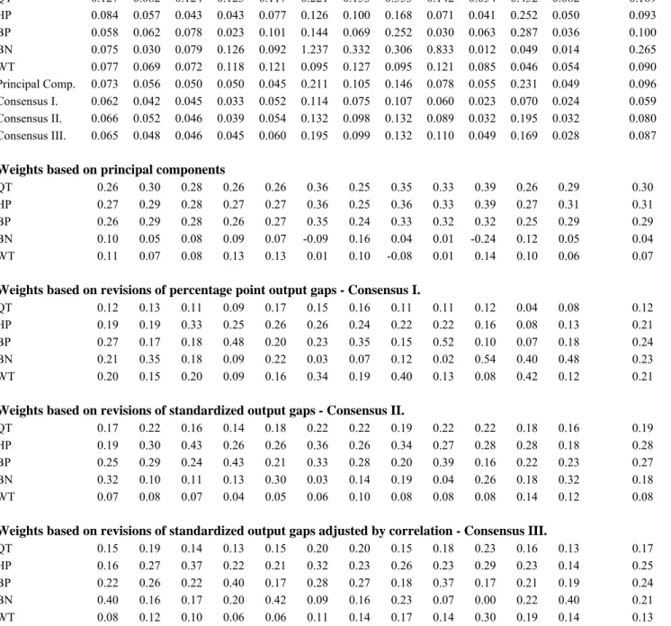
Table 1 reports the revisions of the five individual methods and the four combined methods (principal components, consensus I, consensus II, and consensus III), and the weights derived by the four combined methods. There are several interesting points to highlight.

First, the quadratic time trend tends to have larger revisions than that of the HP, BP, and WT.

The revisions of BN vary substantially across countries, ranging from a fraction of that of the other models in the case of the euro-area to several factors larger than in the cases of Lithuania and Slovakia. The reason behind the small euro-area revision is that in about half of the recursive samples an ARIMA(0,1,2) was found to be the best, which has almost no persistence for the differences. For Lithuania and Slovakia, five and three different models were identified for the recursive samples with nine and six changes in model specifications, respectively. In both countries an ARIMA(4,1,0) was selected the most frequently, which did have considerable persistence for the differences. The wide range of revisions across countries indicates the shakiness of the Beveridge- Nelson decomposition.¹⁹

Second, principal component analysis (PCA) tends to give larger revisions than our combining methods. This result is not merely a consequence of the fact that our weights are based on revisions, since PCA could have attached a large weight to a small revision output gap. Note also that we do not aim to minimize the revisions of the weighted average, but simply base our weights on the reciprocal of the revisions.

18 The sum of the elements of the first eigenvector of principal component analysis was between 1.5 and 2, while the sum of our weights is of course 1. We normalized the weights of the principal component analysis to one for better comparison.

19 Canova (1998) underlines that problems inherent to ARIMA specifications are carried over to the Beveridge-Nelson decomposition. He also states that results of his paper varied considerably with the choice of the lags both in terms of the magnitude of the fluctuations and of the path properties of the data.

Third, in three of the twelve cases PCA attached negative weight to a method. We have already argued that we would expect non-negative weights, since the only prior we have is that each method could give some information about the output gap, but not the inverse of the method could contain this information.

Fourth, results support our consideration that the revisions could be larger for methods revealing larger variance. This effect also reflected in the difference of weights derived from percentage point and standardized output gaps, i.e. the difference between the weights of Consensus I and Consensus II.

Finally, adjusting the weights by the correlation matrix of the individual gaps had only small effects. On average, the weights of the quadratic trend, HP and BP declined somewhat, while BN and WT weights increased by small amounts. We have highlighted that correlation adjustment could lead to negative weights that we exclude. Out of the sixty weights, only one, the BN weight for Slovenia, had such a property, which was set to zero. In this case, mainly WT took over the gap left by the exclusion of the BN output gap.

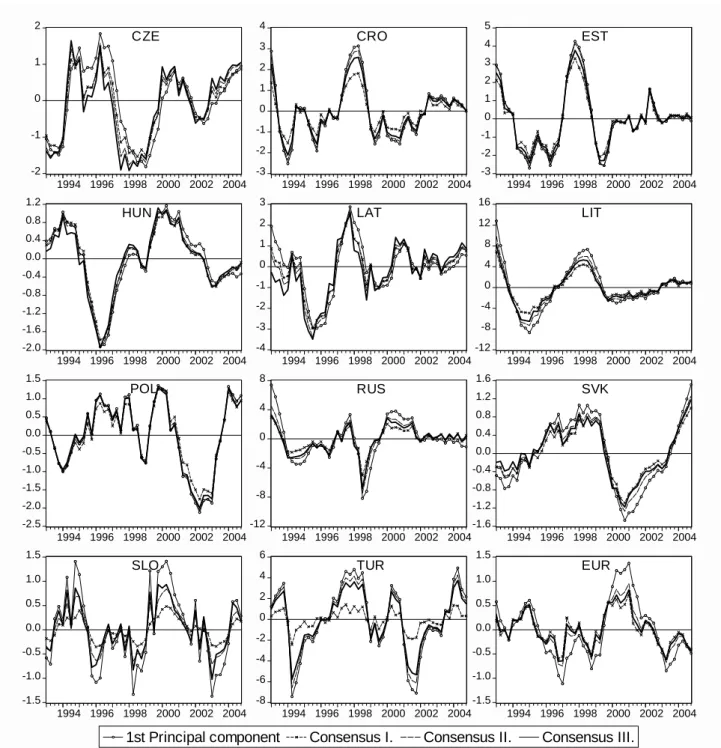
For a graphical inspection, Figure 3 plots the revisions of the five individual methods and three combining methods for the countries studied. In some cases there are indeed quite substantial revisions. For instance, using data up to the end of 2000, the quadratic trend would have indicated that the euro-area economy was at potential at that time. However, using the full sample and the same filter, a 2 percent positive output gap is found for end 2000. Figure 4 plots the full sample estimate of the four combining methods. Generally, the combined gaps do not differ much from each other. Since our method has smaller revisions than that of the PCA and does not allow negative weights, we regard it preferable.

5.2. Application the business cycle correlation analysis

Our weighting method could be used for various purposes, for instance, for business cycle analysis, monetary policy analysis, evaluation of fiscal positions, or optimum currency area (OCA) analysis.

In the topic of monetary policy analysis, Billmeier (2004) and Orphanides-van Norden (2005) study the usefulness of various (individual) output gap measures for forecasting inflation. As an illustration of our combining method, we selected a topic from the OCA literature, as several papers use univariate filters for the study of correlation of business cycles. We are interested in how robust are these results to the specific filter selected.

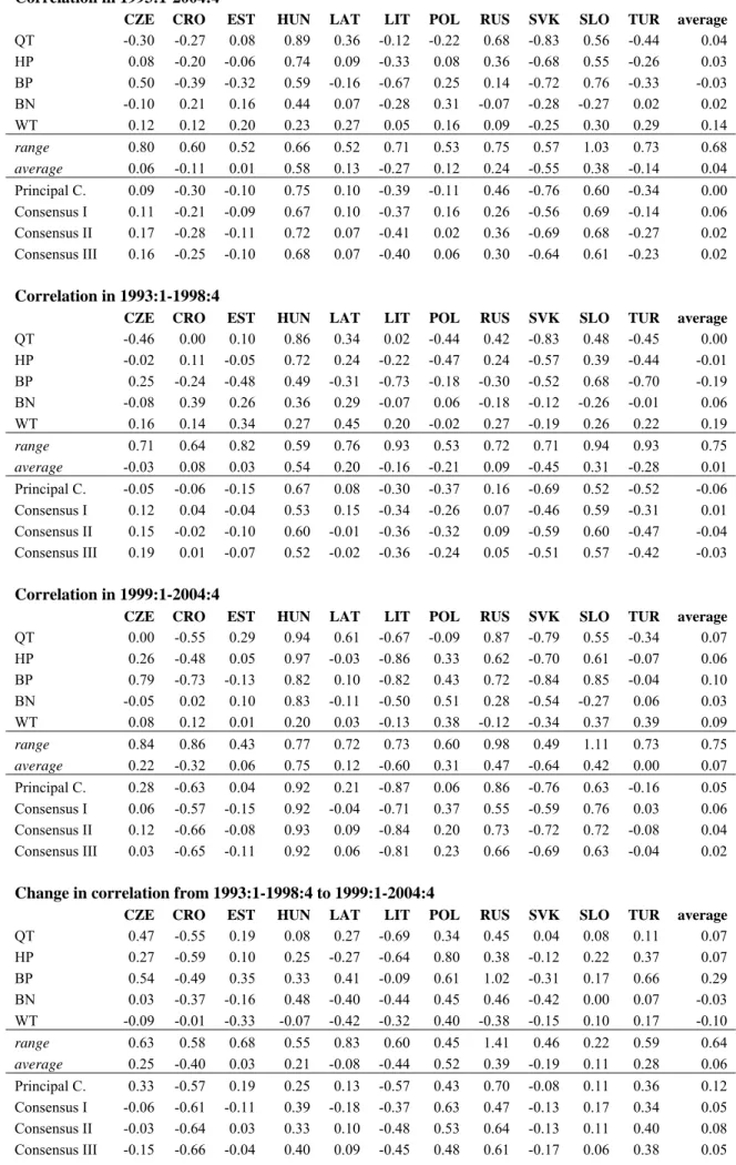
Table 2 reports the correlation coefficient between the business cycles of the euro area and the acceding countries in the full sample period of 1993-2004 and in the first and second 6-year period of this sample. The general conclusion is that different methods reveal rather different conclusions.

For example, in the case of the Czech Republic, in 1999-2004 the quadratic trend and the Beveridge-Nelson decomposition indicate no correlation (0.00 and -0.05), while the BP-filter shows a substantial positive correlation (0.79). The table also shows that the range of correlation coefficients tends to be quite wide, averaging 0.68 in the full sample and 0.75 in both 6-year period sub-samples.

From the perspective of optimum currency union theory not only the level of correlation matters, which, as we have just seen, seems rather different using different methods – the change in

correlation, which tests whether business cycles become synchronized in time, is also important.

This is usually called the test of the ‘endogeneity hypothesis of the OCA’, since these countries became more integrated with the euro area over time. The fourth block of Table 2 reports the change in correlation coefficient from the first to the second sub-period, i.e. the difference between values in the third and the second blocks of the table. The general result, again, is that a conclusion on endogeneity depends heavily on the method and that the conclusions are rather different across methods. The most extreme case is Russia, for which wavelet transformation indicates a 0.38 fall in correlation (from 0.27 to -0.12), while the BP filter indicates a 1.02 increase (from -0.30 to 0.72).

The range between the highest and the smallest changes are also quite wide for other countries (except Slovenia), averaging to 0.64.

To sum up, both the level and the change in correlation coefficients depends heavily on the specific filter adopted.

Among the four combining methods, principal component analysis (PCA) and our measures reveal reasonably similar correlations. The most extreme case is Hungary, for which correlation is 0.92-0.93 in the recent 6-year period using all four combining methods shown in the table. In the case of other countries, variation is somehow larger but we regard them as ‘small’.

Regarding our results for the OCA question, in the second half of the sample Hungary has achieved the highest level of business cycles synchronization (0.92), with Russia and Slovenia coming also to the stage (0.62-0.66), followed by Poland (0.23).²⁰ All other countries are either not correlated (Latvia, Czech Republic, Turkey, and Estonia), or the correlation is even negative, indicating countercyclical movements with the euro area. As for the endogeneity hypothesis, Hungary and Slovenia was already reasonably synchronized in the first half of the sample and among them only Hungary improved by 0.4. Russia and Poland made the biggest improvement (0.61 and 0.48 rise in correlation, respectively). Among the rest of the countries, Turkey made progress from a counter-cyclical position, but in all other countries correlation was either unchanged or even declined in time. This indicates the presence of either important country-specific shocks, or that the transmission of common external shocks is still rather different.

6. Summary

Most of the structural methods for output gap calculations are not applicable to open economies in general and transition countries in particular, and univariate detrending methods are also burdened with various deficiencies. However, univariate methods are frequently used because of the need for detrending for both policy and academic oriented research.

Since all methods have strengths and weaknesses, we do not suggest to pick a single one but to combine individual methods in order to derive a single measure of the output gap. We proposed a new method for combining based on revisions of the output gap for all dates by recursively estimating the models; hence, we suggest giving preference to methods which may lead to more stable inference. Our suggested method also takes into account the variance and the correlation structure of output gaps of individual methods.

20 These results support the findings of Darvas-Szapáry (2005).

We applied our method to business cycles correlation analysis, which has gained considerable interest in the literature. We have shown that results on business cycle correlation of the new EU Member States with the euro area differ substantially according to the method used, which preclude the possibility of drawing firm conclusions. We compared our combining method to principal component analysis. Although the results based on our procedure do not differ much from the results achieved by principal component analysis, our procedure has in many cases much smaller revisions and never derives negative weights, therefore, we regard it preferable.

References

Baxter, M. – King, R. G. (1999): Measuring Business Cycles Approximate Band-pass Filters for Economic Time Series, Review of Economics and Statistics 81, pp. 575-593.

Benczúr, P – Simon, A. – Várpalotai, V. (2002): Dezinflációs számítások kisméretű makromodellel, MNB Working Paper No. 2002/4.

Beveridge, S. – Nelson, C. R. (1981): A New Approach to Decomposition of Economic Time Series into Permanent and Transitory Components with Particular Attention to Measurement of the 'Business Cycle', Journal of Monetary Economics 7, pp. 151-174.

Billmeier, A. (2004): Ghostbusting: Which Output Gap Really Matters? IMF Working Paper 04/146.

Blanchard, O. J. – Quah, D. (1989): The Dynamic Effects of Aggregate Demand and Supply Disturbances, American Economic Review Vol. 79, No. 4, pp. 655-673.

Canova, F. (1998): Detrending and Business Cycle Facts, Journal of Monetary Economics, Vol. 41, pp. 475- 512.

Christiano, Lawrence J. —Fitzgerald, Terry J. (2003): The Band Pass Filter, International Economic Review, 44, No. 2., May 2003, pp.435-65.

Cogley, T. – Nason, J. M. (1995): Effects of the Hodrick-Prescott Filter on Trend and Difference Stationary Time Series: Implications for Business Cycle Research, Journal of Economic Dynamics and Control Vol.

19, pp. 253-278

Cooley, Thomas F. – Mark Dwyer (1998): Business Cycle Analysis without Much Theory: A Look at Structural VARs, Journal of Econometrics 83, 57-88.

Darvas, Zs. – Szapáry, Gy. (2005): Business Cycle Synchronization in the Enlarged EU, CEPR DP No 5179 Darvas, Zs. – Simon, A. (2000): Potential Output and Foreign Trade in Small Open Economies, MNB

Working Paper No. 2000/9.

Daubechies, I. (1988): Orthonormal Bases of Compactly Supported Wavelets, Communication on Pure and Applied Mathematics 41, pp. 909-96.

Denis, C. – McMorrow, K. – Röger Werner (2002): Production function approach to calculating potential growth and output gaps – estimates for the EU Member States and US, Economic Papers No. 176 – September 2002, European Commission.

Dupasquier, C. – Guay, A. – St-Amant, P. (1997): A Comparison of Alternative Methodologies for Estimating Potential Output and the Output Gap, Bank of Canada Working Paper No. 97-5.

Evans, G. – Reichlin, L. (1994): Information, Forecast, and Measurement of the Business Cycle, Journal of Monetary Economics Vol. 33, pp. 233-54.

Faust, J. – Leeper, E. M. (1997): When Do Long-Run Restrictions Give Reliable Results? Journal of Business & Economic Statistics, Vol. 15, No. 3, pp. 345-353.

Fidrmuc, Jarko — Korhonen, Iikka (2004): A meta-analysis of the business cycle correlation between the euro area and the CEECs: What do we know – and who cares? BOFIT Discussion Paper 20/2004.

Gerlach, S. – Smets, F. (1999): Output Gaps and Monetary Policy in the EMU Area, European Economic Review, Vol. 43, pp.801-812.

Giorno, C. – Richardson, P. – Roseveare, Deborah – van den Noord, Paul (1995): Estimating Potential Output, Output Gaps and Structural Budget Balances, OECD Economics Department Working Papers No. 152.

Harvey, A.C. – Jaeger, A. (1993): Detrending, Stylized Facts and the Business Cycle, Journal of Applied Econometrics 8, pp. 231-47.

Harvey, A.C. (1989): Forecasting, Structural Time Series Models, and the Kalman Filter, Cambridge U.K.:

Cambridge University Press.

Hodrick, R. J. – Prescott, E. C. (1997): Postwar US Business Cycles: An Empirical Investigation, Journal of Money, Credit, and Banking, Vol. 29, pp. 1-16.

Kuttner, K. N. (1994): Estimating Potential Output as a Latent Variable, Journal of Business & Economic Statistics, Vol. 12, No. 3, pp.361-368.

Lippi, M. – Reichlin, L. (1994): Diffusion of Technical Change and the Decomposition of Output into Trend and Cycle, Review of Economic Studies 61, pp. 19-30.

Orphanides, A. van Norden, S. (2002): The Unreliability of Output Gap Estimates in Real Time, Review of Economics and Statistics 84, pp. 569-583.

Orphanides, A. van Norden, S. (2005): The Reliability of Inflation Forecasts Based on Output Gap Estimates in Real Time, CEPR Discussion Paper 4830.

Percival, D. B. – Walden, A. T. (2000): Wavelet Methods for Time Series Analysis, Cambridge University Press.

Schleicher, C. (2002): An Introduction to Wavelets for Economists, Bank of Canada, Working Paper No.

2002-3.

Smets, Frank — Wouters, Raf (2003): Output gaps: Theory versus practice, paper presented at the ASSA Meetings in Washington, D.C, January 2003.

Stiglitz, J.E. (1992): Capital Markets and Economic Fluctuations in Capitalist Economies, European Economic Review 36, 269-306.

Stock, James H. — Mark O. W. Watson (1999): Business Cycle Fluctuations in US Macroeconomic Time Series, in Handbook of Macroeconomics, Vol. 1., Edited by J.B. Taylor and M. Woodford, Elseiver Science B.V., pp. 3-64.

Várpalotai, V. (2003): Numerical method for backward projection of macroeconomic data, MNB Working Paper 2003/2.

Watson, M.W. (1986): Univariate Detrending Methods with Stochastic Trends, Journal of Monetary Economics 18, pp. 49-75.

Figure 1 Inflation and unemployment rate, 1993Q1-2004Q4

0 10 20 30 40 50

0 10 20 30 40 50

94 95 96 97 98 99 00 01 02 03 04

CPI

0 4 8 12 16 20

0 4 8 12 16 20

94 95 96 97 98 99 00 01 02 03 04 Czech Rep.

Croatia Estonia

Hungary Latvia Lithuania

Poland Russia Slovak Rep.

Slovenia Turkey Euro-area

U

Figure 2 Annual growth of GDP, 1994Q1-2004Q4

-15 -10 -5 0 5 10 15

-15 -10 -5 0 5 10 15

94 95 96 97 98 99 00 01 02 03 04 Estonia

Latvia Lithuania

Turkey Croatia Russia

-2 0 2 4 6 8

-2 0 2 4 6 8

94 95 96 97 98 99 00 01 02 03 04 Czech Rep.

Hungary Poland

Slovak Rep.

Slovenia Euro-area

Figure 3 Revisions (estimations for recursive samples)

Notes for Figure 3. QT: quadratic trend, HP: Hodrick-Prescott filter, BP: band-pass filter, BN: Beveridge-Nelson decomposition, WT: wavelet transformation. Principal Comp.: combined output gap measure by the principal component analysis. Consensus I:

combined output gap measure using equations (1), (2), (3), and (4). Consensus III: combined output gap measure using equations (1’’), (2), (3), and (4).

-3 -2 -1 0 1 2 3 4

93 94 95 96 97 98 99 00 01 02 03 04

CZE QT

-3 -2 -1 0 1 2 3

93 94 95 96 97 98 99 00 01 02 03 04

CZE HP

-3 -2 -1 0 1 2

93 94 95 96 97 98 99 00 01 02 03 04

CZE BP

-5 -4 -3 -2 -1 0 1 2 3 4

93 94 95 96 97 98 99 00 01 02 03 04

CZE BN

-1.2 -0.8 -0.4 0.0 0.4 0.8 1.2

93 94 95 96 97 98 99 00 01 02 03 04

CZE WT

-2 -1 0 1 2

93 94 95 96 97 98 99 00 01 02 03 04

CZE 1st Principal Comp.

-1.6 -1.2 -0.8 -0.4 0.0 0.4 0.8 1.2 1.6

93 94 95 96 97 98 99 00 01 02 03 04

CZE Consensus I.

-2 -1 0 1 2

93 94 95 96 97 98 99 00 01 02 03 04

CZE Consensus III.

Czech Republic: Revisions

-6 -4 -2 0 2 4 6

93 94 95 96 97 98 99 00 01 02 03 04

CRO QT

-3 -2 -1 0 1 2 3 4 5

93 94 95 96 97 98 99 00 01 02 03 04

CRO HP

-4 -3 -2 -1 0 1 2 3 4 5

93 94 95 96 97 98 99 00 01 02 03 04

CRO BP

-2 -1 0 1 2

93 94 95 96 97 98 99 00 01 02 03 04

CRO BN

-1.2 -0.8 -0.4 0.0 0.4 0.8 1.2

93 94 95 96 97 98 99 00 01 02 03 04

CRO WT

-3 -2 -1 0 1 2 3 4

93 94 95 96 97 98 99 00 01 02 03 04

CRO 1st Principal Comp.

-2.0 -1.5 -1.0 -0.5 0.0 0.5 1.0 1.5 2.0

93 94 95 96 97 98 99 00 01 02 03 04

CRO Consensus I.

-3 -2 -1 0 1 2 3

93 94 95 96 97 98 99 00 01 02 03 04

CRO Consensus III.

Croatia: Revisions

-3 -2 -1 0 1 2

93 94 95 96 97 98 99 00 01 02 03 04

HUN QT

-3 -2 -1 0 1 2 3

93 94 95 96 97 98 99 00 01 02 03 04

HUN HP

-2.0 -1.6 -1.2 -0.8 -0.4 0.0 0.4 0.8 1.2

93 94 95 96 97 98 99 00 01 02 03 04

HUN BP

-6 -4 -2 0 2 4

93 94 95 96 97 98 99 00 01 02 03 04

HUN BN

-1.2 -0.8 -0.4 0.0 0.4 0.8 1.2

93 94 95 96 97 98 99 00 01 02 03 04

HUN WT

-2.0 -1.5 -1.0 -0.5 0.0 0.5 1.0 1.5

93 94 95 96 97 98 99 00 01 02 03 04

HUN 1st Principal Comp.

-2.0 -1.5 -1.0 -0.5 0.0 0.5 1.0 1.5

93 94 95 96 97 98 99 00 01 02 03 04

HUN Consensus I.

-3 -2 -1 0 1 2

93 94 95 96 97 98 99 00 01 02 03 04

HUN Consensus III.

Hungary: Revisions

-4 -3 -2 -1 0 1 2 3 4

93 94 95 96 97 98 99 00 01 02 03 04

LAT QT

-4 -3 -2 -1 0 1 2 3 4 5

93 94 95 96 97 98 99 00 01 02 03 04

LAT HP

-4 -3 -2 -1 0 1 2 3 4

93 94 95 96 97 98 99 00 01 02 03 04

LAT BP

-6 -4 -2 0 2 4 6

93 94 95 96 97 98 99 00 01 02 03 04

LAT BN

-1.2 -0.8 -0.4 0.0 0.4 0.8 1.2

93 94 95 96 97 98 99 00 01 02 03 04

LAT WT

-3 -2 -1 0 1 2 3 4

93 94 95 96 97 98 99 00 01 02 03 04

LAT 1st Principal Comp.

-3 -2 -1 0 1 2 3

93 94 95 96 97 98 99 00 01 02 03 04

LAT Consensus I.

-4 -3 -2 -1 0 1 2 3 4

93 94 95 96 97 98 99 00 01 02 03 04

LAT Consensus III.

Latvia: Revisions

-10 -5 0 5 10 15

93 94 95 96 97 98 99 00 01 02 03 04

LIT QT

-10 -5 0 5 10 15

93 94 95 96 97 98 99 00 01 02 03 04

LIT HP

-12 -8 -4 0 4 8

93 94 95 96 97 98 99 00 01 02 03 04

LIT BP

-40 -30 -20 -10 0 10

93 94 95 96 97 98 99 00 01 02 03 04

LIT BN

-1.2 -0.8 -0.4 0.0 0.4 0.8 1.2

93 94 95 96 97 98 99 00 01 02 03 04

LIT WT

-10 -5 0 5 10 15

93 94 95 96 97 98 99 00 01 02 03 04

LIT 1st Principal Comp.

-6 -4 -2 0 2 4 6 8

93 94 95 96 97 98 99 00 01 02 03 04

LIT Consensus I.

-8 -4 0 4 8 12

93 94 95 96 97 98 99 00 01 02 03 04

LIT Consensus III.

Lithuania: Revisions

-3 -2 -1 0 1 2 3 4

93 94 95 96 97 98 99 00 01 02 03 04

POL QT

-3 -2 -1 0 1 2

93 94 95 96 97 98 99 00 01 02 03 04

POL HP

-2.0 -1.5 -1.0 -0.5 0.0 0.5 1.0 1.5 2.0

93 94 95 96 97 98 99 00 01 02 03 04

POL BP

-8 -4 0 4 8 12

93 94 95 96 97 98 99 00 01 02 03 04

POL BN

-1.2 -0.8 -0.4 0.0 0.4 0.8 1.2

93 94 95 96 97 98 99 00 01 02 03 04

POL WT

-3 -2 -1 0 1 2

93 94 95 96 97 98 99 00 01 02 03 04

POL 1st Principal Comp.

-2.0 -1.5 -1.0 -0.5 0.0 0.5 1.0 1.5

93 94 95 96 97 98 99 00 01 02 03 04

POL Consensus I.

-3 -2 -1 0 1 2

93 94 95 96 97 98 99 00 01 02 03 04

POL Consensus III.

Poland: Revisions