The Q measureanditsconnectionswithbelief,probability,plausibility,roughsets,multiattributeutilityfunctionsandfuzzyoperators The λ -additiveMeasureinaNewLight

(will be inserted by the editor)

The λ -additive Measure in a New Light

The Q

measure and its connections with belief, probability, plausibility, rough sets, multiattribute utility functions and fuzzy operators

J´ozsef Dombi · Tam´as J´on´as

Received: date / Accepted: date

Abstract The aim of this paper is twofold. On the one hand, theλ-additive measure (Sugenoλ-measure) is revisited and a state-of-the-art summary of its most important properties is provided. On the other hand, the so-calledν-additive mea- sure as an alternatively parameterizedλ-additive measure is introduced. Here, the advantages of theν-additive measure are discussed and it is demonstrated that these two mea- sures are closely related to various areas of science. The motivation for introducing theν-additive measure lies in the fact that its parameterν∈(0,1)has an important semantic meaning as it is the fix point of the complement operation.

Here, by utilizing theν-additive measure, some well-known results concerning theλ-additive measure are put into a new light and rephrased in more advantageous forms. It is dis- cussed here how theν-additive measure is connected with the belief-, probability- and plausibility measures. Next, it is also shown that twoν-additive measures, with the parame- tersν1andν2, are a dual pair of belief- and plausibility mea- sures if and only ifν₁+ν₂=1. Furthermore, it is demon- strated how aν-additive measure (or aλ-additive measure) can be transformed to a probability measure and vice versa.

Lastly, it is discussed here how theν-additive measures are connected with rough sets, multi-attribute utility functions and with certain operators of fuzzy logic.

Keywords belief·probability·plausibility·λ-additive measure·rough sets·multi-attribute utility functions

J´ozsef Dombi

Institute of Informatics, University of Szeged, Szeged, Hungary E-mail: dombi@inf.u-szeged.hu Tam´as J´on´as

Institute of Business Economics, E¨otv¨os Lor´and University, Budapest, Hungary E-mail: jonas@gti.elte.hu

Corresponding author, tel: +36 30 688 5651

1 Introduction

It is an acknowledged fact that the λ-additive measure (Sugeno λ-measure) (Sugeno 1974) is one of the most widely applied monotone measure (fuzzy measure). The usefulness, versatility and applicability ofλ-additive mea- sures has inspired numerous theoretical and practical re- searches since Sugeno’s original results were published in 1974 (see, e.g. Magadum and Bapat (2018); Mohamed and Xiao (2003); Chit¸escu (2015); Chen et al. (2016); Singh (2018)).

The aim of the present study is twofold. On the one hand, we will revisit theλ-additive measure and give a state-of- the-art summary of its most important properties. On the other hand, we will introduce the so-calledν-additive mea- sure as an alternatively parameterizedλ-additive measure, demonstrate the advantages of theν-additive measure and point out that these two measures are closely related to var- ious areas of science. The motivation for introducing theν- additive measure lies in the fact that its parameterν∈(0,1) has an important semantic meaning. Namely, ν is the fix point of the complement operation; that is, if theνadditive measure of a set has the valueν, then theν-additive measure of its complement set has the valueνas well. It should be added that by utilizing theν-additive measure, some well- known results concerning theλ-additive measure can be put into a new light and rephrased in more advantageous forms.

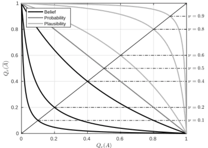
Here, we will discuss how the ν-additive measure is con- nected with the belief-, probability- and plausibility mea- sures (see, e.g. Wang and Klir (2013); H¨ohle (1987); Dubois and Prade (1980); Spohn (2012); Feng et al. (2014)). Also, we will demonstrate that aν-additive measure is a

(1) belief measure if and only if 0<ν≤1/2 (2) probability measure if and only ifν=1/2 (3) plausibility measure if and only if 1/2≤ν<1.

Next, we will show that two ν-additive measures, with the parameters ν₁ and ν₂, are a dual pair of belief- and plausibility measures if and only if ν1+ν2=1. Further- more, we will discuss how a ν-additive measure (or a λ- additive measure) can be transformed to a probability mea- sure and vice versa. Moreover, we will also discuss how theν-additive measures are connected with rough sets (see, e.g. Dubois and Prade (1990); Yao and Lingras (1998); Wu et al. (2002); Polkowski (2013)), multi-attribute utility func- tions (see, e.g. Sarin (2013); Greco et al. (2016); Keeney and Raiffa (1993)), and with certain operators of continuous- valued logic (see, e.g. Dombi (1982, 2008)).

The rest of this paper is structured as follows. In Section 2, we give an overview of the monotone (fuzzy) measures in- cluding the belief-, probability- and plausibility measures. In Section 3, theν-additive measure is introduced and its key properties are discussed. In Section 4, we demonstrate how theν-additive measure is related to the belief-, probability- and plausibility measures, and in Section 5, we show how a ν-additive measure can be transformed to a probability mea- sure and vice versa. Section 6 reveals some areas of science which the ν-additive (λ-additive) measures are connected with. Lastly, in Section 7, we give a short summary of our findings and highlight our future research plans including the possible application of ν-additive measure in network science.

In this study, we will use the common notations∩and∪ for the intersection and union operations over sets, respec- tively. Also, will use the notationAfor the complement of setA.

2 Monotone measures

Now, we will introduce the monotone measures and give a short overview of them that covers the probability-, belief- and plausibility measures.

Definition 1 LetΣ be aσ-algebra on the set X. Then the functiong:Σ→[0,1]is a monotone measure on the measur- able space(X,Σ)iffgsatisfies the following requirements:

(1) g(/0) =0,g(X) =1

(2) ifB⊆A, theng(B)≤g(A)for anyA,B∈Σ(monotonic- ity)

(3) if∀i∈N,A_i∈Σand(A_i)is monotonic(A₁⊆A2⊆. . .⊆ A_n⊆. . .orA₁⊇A₂⊇. . .⊇A_n. . .), then

i→∞limg(A_i) =g

i→∞limAi

(continuity).

IfX is a finite set, then the continuity requirement in Definition 1 can be disregarded and the monotone measure is defined as follows.

Definition 2 The functiong:P(X)→[0,1]is a monotone measure on the finite setX iffg satisfies the following re- quirements:

(1) g(/0) =0,g(X) =1

(2) ifB⊆A, theng(B)≤g(A)for anyA,B∈P(X)(mono- tonicity).

Note that the monotone measures given by Definition 1 and Definition 2 are known as fuzzy measures, which were originally defined by Choquet (Choquet 1954) and Sugeno (Sugeno 1974).

2.1 Some examples of monotone measures 2.1.1 Dirac measure

Definition 3 The functionδx₀ :P(X)→[0,1] is a Dirac measure on the setX, iff∀A∈P(X):

δx₀(A) =

(1, ifx₀∈A 0, otherwise.

2.1.2 Probability measure

Definition 4 LetΣbe aσ-algebra over the setX. Then the functionPr:Σ→[0,1]is a probability measure on the space (X,Σ)iffPrsatisfies the following requirements:

(1) ∀A∈Σ:Pr(A)≥0 (2) Pr(X) =1

(3) ∀A₁,A₂, . . .∈Σ, ifA_i∩A_j=/0,∀i6= j, then Pr

∞ [

i=1

A_i

!

=

∞ i=1

∑

Pr(A_i).

Remark 1 IfXis a finite set, then requirement (3) in Defini- tion 4 can be reduced to the following requirement: for any disjointA,B∈P(X),Pr(A∪B) =Pr(A) +Pr(B).

2.1.3 Belief measure and plausibility measure

Definition 5 The function Bl :P(X)→[0,1] is a belief measure on the finite setX, iffBlsatisfies the following re- quirements:

(1) Bl(/0) =0,Bl(X) =1

(2) for anyA1,A2, . . . ,An∈P(X), Bl(A₁∪A₂∪ · · · ∪A_n)≥

≥

n

∑

k=1

∑

1≤i₁<i2···

···<i_k≤n

(−1)^k−1Bl A_i1∩A_i1∩ · · · ∩A_ik

. (1)

Here,Bl(A)is interpreted as a grade of belief in that a given element ofXbelongs toA.

Lemma 1 If Bl is a belief measure on the finite set X , then for any A∈P(X),

Bl(A) +Bl(A)≤1.

Proof Noting Definition 5, we have

1=Bl(A∪A)≥Bl(A) +Bl(A)−Bl(A∩A) =Bl(A) +Bl(A).

u t The inequalityBl(A) +Bl(A)≤1 means that a lack of belief inx∈Adoes not imply a strong belief inx∈A. In particular, total ignorance is modeled by the belief function Bl_isuch thatBl_i(A) =0 ifA6=XandBl_i(A) =1 ifA=X.

The following proposition is about the monotonicity of belief measures.

Proposition 1 If X is a finite set, Bl is a belief measure on X , A,B∈P(X)and B⊆A, then Bl(B)≤Bl(A).

Proof LetB⊆A. Hence, there existsC∈P(X)such that A=B∪CandB∩C=/0. Now, by utilizing the definition of the belief measure and the fact thatB∩C=/0, we get Bl(A) =Bl(B∪C)≥Bl(B) +Bl(C)≥Bl(B).

u t Corollary 1 The belief measure given by Definition 5 is a monotone measure.

Proof LetBl be a belief measure. It follows from Defini- tion 5 thatBlsatisfies criterion (1) for a monotone measure given in Definition 2. Moreover, the monotonicity ofBlwas proven in Proposition 1; that is,Blalso satisfies criterion (2)

in Definition 2. ut

Definition 6 The functionPl:P(X)→[0,1]is a plausibil- ity measure on the finite setX, iffPl satisfies the following requirements:

(1) Pl(/0) =0,Pl(X) =1

(2) for anyA₁,A₂, . . . ,A_n∈P(X), Pl(A₁∩A₂∩ · · · ∩A_n)≤

≤

n

∑

k=1

∑

1≤i₁<i2···

···<i_k≤n

(−1)^k−1Pl A_i1∪A_i2· · · ∪A_ik

. (2)

Here,Pl(A)is interpreted as the plausibility ofA.

Lemma 2 If Pl is a plausibility measure on the finite set X , then for any A∈P(X),

Pl(A) +Pl(A)≥1.

Proof Noting Definition 6, we have

0=Pl(A∩A)≤Pl(A) +Pl(A)−Pl(A∪A) =

=Pl(A) +Pl(A)−1,

from whichPl(A) +Pl(A)≥1 follows. ut This result can be interpreted so that the plausibility ofx∈A does not imply a strong plausibility ofx∈A.

The following proposition is about the monotonicity of plausibility measures.

Proposition 2 If X is a finite set, Pl is a plausibility measure on X , A,B∈P(X)and B⊆A, then Pl(B)≤Pl(A).

Proof LetB⊆A. LetC∈P(X)such thatA∩C=Band A∪C=X. Now, by utilizing the definition of plausibility measure, and the facts thatA∪C=XandPl(C)≤1, we get Pl(B) =Pl(A∩C)≤Pl(A) +Pl(C)−Pl(A∪C) =

=Pl(A) +Pl(C)−1≤Pl(A).

u t Corollary 2 The plausibility measure given by Definition 6 is a monotone measure.

Proof LetPlbe a plausibility measure. It follows from Def- inition 6 thatPl satisfies criterion (1) for a monotone mea- sure given in Definition 2. Next, the monotonicity ofPlwas proven in Proposition 2; that is,Plalso satisfies criterion (2)

in Definition 2. ut

The plausibility of a subsetAof the finite setX was de- fined by Shafer (Shafer 1976) as

Pl(A) =1−Bl(A),

where Bl is a belief function. The following proposition states an interesting connection between the belief measure and the plausibility measure.

Proposition 3 Let X be a finite set and letµ1,µ2:P(X)→ [0,1]be two monotone measures on X such that

µ2(A) =1−µ1(A) (3)

holds for any A∈P(X). Then, either (1)µ1is a belief mea- sure on X if and only ifµ2is a plausibility measure on X , or (2)µ₁is a plausibility measure on X if and only ifµ₂is a belief measure on X .

Proof We will prove case (1), and the proof of case (2) is similar. Firstly, we will show that if µ1 is a belief mea- sure on X and µ₂(A) is given as µ₂(A) =1−µ₁(A) for any A∈P(X), then µ2 is a plausibility measure on X.

Let µ1 be a belief measure on X and µ2(A) =1−µ1(A)

for any A∈P(X). Then,µ2(/0) =0 andµ2(X) =1 triv- ially follow from the fact that µ₁is a belief measure and µ2(A) =1−µ₁(A). That is, functionµ2satisfies requirement (1) for a plausibility measure given in Definition 6. Further- more, since functionµ₁is a belief measure, the inequality

µ1(A₁∪A₂∪ · · · ∪A_n)≥

≥

n

∑

k=1

∑

1≤i₁<i₂···<i_k≤n

(−1)^k−1µ₁ A_i1∩A_i1∩ · · · ∩A_ik

. (4)

holds for any A1,A2, . . . ,An∈P(X). From the condition µ2(A) =1−µ1(A), we also have that µ1(A) =1−µ2(A).

Next, applying the inequality in Eq. (4) to the comple- ment setsA1,A2, . . . ,An∈P(X)and utilizing the fact that µ1(A) =1−µ2(A), we get

1−µ₂(A₁∪A₂∪ · · · ∪A_n)≥

≥1−µ2(A₁) +1−µ2(A₂) +· · ·+1−µ2(A_n)−

−(1−µ2(A₁∩A₂))− · · · −(1−µ2(An−1∩A_n)) +· · ·

· · ·+ (−1)ⁿ⁺¹

1−µ₂(A₁∩A₂∩ · · · ∩A_n)

=

=−µ₂(A₁)−µ2(A₂)− · · · −µ2(A_n)+

+µ₂(A₁∩A₂) +· · ·+µ2(An−1∩A_n) +· · ·

· · ·+ (−1)ⁿµ2(A₁∩A2∩ · · · ∩A_n)+

+ n

1

− n

2

+· · ·+ n

n

(−1)ⁿ⁺¹. Noting the fact that

n

∑

k=1

n k

(−1)^k+1=1, (5)

the previous inequality can be written as 1−µ2(A₁∪A₂∪ · · · ∪A_n)≥

≥1−µ2(A₁)−µ2(A₂)− · · · −µ2(A_n)+

+µ₂(A₁∩A₂) +· · ·+µ2(An−1∩A_n) +· · ·

· · ·+ (−1)ⁿµ₂(A₁∩A₂∩ · · · ∩A_n).

Now, applying the De Morgan law to the last inequality, we get

µ2(A₁∩A₂∩ · · · ∩A_n)≤

≤

n

k=1

∑ ∑

1≤i₁<i₂···<i_k≤n

(−1)^k−1µ2 A_i1∪A_i1∪ · · · ∪A_ik , which means that functionµ2is a plausibility measure.

Secondly, we will demonstrate that ifµ2is a plausibility measure onX andµ2(A)is given asµ2(A) =1−µ1(A)for anyA∈P(X), thenµ₁is a belief measure onX. Letµ₂be a plausibility measure onX andµ2(A) =1−µ1(A)for any A∈P(X). These conditions trivially imply thatµ1(/0) =0

andµ1(X) =1; that is, functionµ1satisfies requirement (1) for a belief measure given in Definition 5. Next, because functionµ2is a plausibility measure, the inequality

µ₂(A₁∩A₂∩ · · · ∩A_n)≤

≤

n

∑

k=1

∑

1≤i₁<i2···<i_k≤n

(−1)^k−1µ₂ A_i1∪A_i2· · · ∪A_ik (6) holds for anyA₁,A₂, . . . ,A_n∈P(X). Then, applying the in- equality in Eq. (6) to the complement setsA₁,A₂, . . . ,A_n∈ P(X)and utilizing the condition that µ₂(A) =1−µ₁(A), we get

1−µ₁(A₁∩A₂∩ · · · ∩A_n)≤

≤1−µ1(A₁) +1−µ1(A₂) +· · ·+1−µ1(A_n)−

−(1−µ1(A₁∪A₂))− · · · −(1−µ1(An−1∪A_n)) +· · ·

· · ·+ (−1)ⁿ⁺¹

1−µ₁(A₁∪A₂∪ · · · ∪A_n)

=

=−µ₁(A₁)−µ1(A₂)− · · · −µ1(A_n)+

+µ₁(A₁∪A₂) +· · ·+µ1(An−1∪A_n) +· · ·

· · ·+ (−1)ⁿµ1(A₁∪A2∪ · · · ∪A_n)+

+ n

1

− n

2

+· · ·+

n n

(−1)ⁿ⁺¹.

Again, taking into account Eq. (5), the previous inequality can be written as

1−µ1(A₁∩A₂∩ · · · ∩A_n)≤

≤1−µ₁(A₁)−µ₁(A₂)− · · · −µ₁(A_n)+

+µ₁(A₁∪A2) +· · ·+µ1(A_n−1∪An) +· · ·

· · ·+ (−1)ⁿµ1(A₁∪A₂∪ · · · ∪A_n).

Now, applying the De Morgan law to the last inequality, we get

µ1(A₁∪A₂∪ · · · ∪A_n)≥

≥

n

∑

k=1

∑

1≤i₁<i2···<i_k≤n

(−1)^k−1µ₁ A_i1∩A_i1∩ · · · ∩A_ik .

Hence,µ1is a belief measure. ut

Later, we will use the concept of dual pair of belief- and plausibility measures.

Definition 7 LetBlandPlbe a belief measure and a plau- sibility measure, respectively, on setX. ThenBlandPl are said to be a dual pair of belief- and plausibility measures iff Pl(A) =1−Bl(A)

holds for anyA∈P(X).

In the Dempster-Shafer theory of evidence, a belief mass is assigned to each element of the power setP(X), whereX is a finite set. The belief mass is given by the so-called basic probability assignmentmfromP(X)to[0,1]that is defined as follows.

Definition 8 The function m:P(X)→[0,1] is a basic probability assignment (mass function) on the finite setX, iffmsatisfies the following requirements:

(1) m(/0) =0

(2) ∑A∈P(X)m(A) =1.

The subsetsAofX for whichm(A)>0 are called the focal elements of m. Let x∈A andA∈P(X). Then, the mass m(A)can be interpreted as the probability of knowingx∈A given the available evidence. Utilizing a given basic proba- bility assignmentm, the beliefBl(A)for the setAis Bl(A) =

∑

B|B⊆A

m(B),

and the plausibilityPl(A)is Pl(A) =

∑

B|B∩A6=/0

m(B).

A basic probability assignmentmcan be represented by its belief functionBlas

m(B) =

∑

A⊆B

(−1)^|B\A|Bl(A),

whereB∈P(X). Here,mis the basic probability assign- ment of the belief measureBl. Note that plausibility mea- sures and belief functions were introduced by Dempster Dempster (1967) under the names upper and lower proba- bilities, induced by a probability measure by a multivalued mapping.

Remark 2 The monotonicity of the plausibility measurePl can also be demonstrated by utilizing the duality Pl(A) = 1−Bl(A)and the monotonicity of the belief measure Bl. Namely, ifB⊆A, thenA⊆Band so

Bl(A)≤Bl(B), from which

1−Bl(A)≥1−Bl(B), which means that Pl(A)≥Pl(B).

3 Introduction to theQ_νmeasure

Relaxing the additivity property of the probability measure, theλ-additive measures were proposed by Sugeno in 1974 (Sugeno 1974).

Definition 9 The function Q_λ : P(X)→ [0,1] is a λ- additive measure (Sugeno λ-measure) on the finite set X, iffQ_λ satisfies the following requirements:

(1) Q_λ(X) =1

(2) for anyA,B∈P(X)andA∩B=/0,

Q_λ(A∪B) =Q_λ(A) +Q_λ(B) +λQ_λ(A)Q_λ(B), (7) whereλ ∈(−1,∞).

Note that if X is an infinite set, then the continuity of functionQ_λ is also required. Here, we will show that the λ-additive measures are monotone measures as well.

Proposition 4 Every λ-additive measure is a monotone measure.

Proof LetQ_λ be aλ-additive measure on the setX. Then Q_λ(X) =1 holds by definition. Next, by utilizing Eq. (7), we get Q_λ(X) =Q_λ(X∪/0) =Q_λ(X) +Q_λ(/0)(1+λQ_λ(X)), which implies thatQ_λ(/0) =0. Thus,Q_λ satisfies criterion (1) of a monotone measure given in Definition 2.

Next, letA,B∈P(X)and letB⊆A. Then there exists aC∈P(X)such thatA=B∪CandB∩C=/0. Now, by utilizing Eq. (7) and the fact thatλ>−1, we get

Q_λ(A) =Q_λ(B∪C) =

=Q_λ(B) +Q_λ(C)(1+λQ_λ(B))≥Q_λ(B).

It means thatQ_λ also satisfies the monotonicity criterion of

a monotone measure. ut

Remark 3 The requirementλ ≥ −1 instead of the require- mentλ>−1 would be sufficient to ensure the monotonicity ofQ_λ (see Proposition 4). The requirementλ≥ −1 also en- sures that for anyA,B∈P(X)andA∩B=/0 theQ_λ(A∪B) quantity is non-negative. Namely, since Q_λ(A),Q_λ(B)∈ [0,1], the inequality

Q_λ(A)Q_λ(B)≤p

Q_λ(A)Q_λ(B)≤Q_λ(A) +Q_λ(B) holds, and so ifλ≥ −1, then

0≤(1+λ)Q_λ(A)Q_λ(B) =

=Q_λ(A)Q_λ(B) +λQ_λ(A)Q_λ(B)≤

≤Q_λ(A) +Q_λ(B) +λQ_λ(A)Q_λ(B) =Q_λ(A∪B).

However, the requirementλ >−1 is given in the definition ofλ-additive measures. Later, we will see that certain prop- erties ofλ-additive measures hold only ifλ >−1.

3.1 Theλ-additive complement and the Dombi form of negation

Proposition 5 If X is a finite set and Q_λ is a λ-additive measure on X , then for any A∈P(X)the Q_λ measure of the complement set A=X\A is

Q_λ(A) = 1−Q_λ(A)

1+λQ_λ(A). (8)

Proof SinceA∩A=/0, we can write 1=Q_λ(X) =Q_λ(A∪A) =

=Q_λ(A) +Q_λ(A) +λQ_λ(A)Q_λ(A) =

=Q_λ(A) +Q_λ(A)(1+λQ_λ(A)), from which we get

Q_λ(A) = 1−Q_λ(A) 1+λQ_λ(A).

u t Remark 4 For anyA∈P(X), we have

Q_λ(A) +Q_λ(A) =Q_λ(A) + 1−Q_λ(A) 1+λQ_λ(A)=

=1+λQ²

λ(A)

1+λQ_λ(A)=1−λQ_λ(A)Q_λ(A).

(9)

It can be seen from Eq. (9) that

0<Q_λ(A) +Q_λ(A)≤1 if λ ∈(0,∞) Q_λ(A) +Q_λ(A) =1 if λ =0 1≤Q_λ(A) +Q_λ(A)<2 if λ ∈(−1,0).

We have shown in Proposition 5 that ifX is a finite set andQ_λis aλ-additive measure onX, then for anyA∈P(X) theQ_λ measure of the complement setA=X\Ais Q_λ(A) = 1−Q_λ(A)

1+λQ_λ(A). (10)

Now, let us assume that 0≤Q(A)<1. Then, Eq. (10) can be written as

Q_λ(A) = 1−Q_λ(A)

1+λQ_λ(A)= 1 1+ (1+λ)_1−Q^Qλ(A)

λ(A)

. (11)

In continuous-valued logic, the Dombi form of negation with the neutral value ν ∈(0,1)is given by the operator nν:[0,1]→[0,1]as follows:

n_ν(x) =







1

1+(^1−ν_ν )²_1−x^x ifx∈[0,1)

0 ifx=1,

(12) where x ∈ [0,1] is a continuous-valued logic variable (Dombi 2008). Note that the Dombi form of negation is the unique Sugeno’s negation (Sugeno 1993) with the fix

pointν∈(0,1). Also, forQ_λ(A)∈[0,1), the formula ofλ- additive measure ofQ_λ(A)in Eq. (11) is the same as the formula of the Dombi form of negation in Eq. (12) with x=Q_λ(A)and

1−ν ν

2

=1+λ.

Based on the definition ofλ-additive measures,λ>−1, and since

λ= 1−ν

ν 2

−1

is a bijection between (0,1) and (−1,∞), the λ-additive measure of the complement setA can be alternatively re- defined as

Q_λ(A) =







1 1+(^1−ν_ν )²_1−Q^Qλ(A)

λ(A)

ifQ_λ(A)∈[0,1)

0 ifQ_λ(A) =1,

(13)

where ^1−ν_ν 2

=1+λ,ν∈(0,1).

Following this line of thinking, here, we will introduce theν-additive measure and state some of its properties.

Definition 10 The function Q_ν :P(X)→ [0,1] is a ν- additive measure on the finite setX, iffQ_νsatisfies the fol- lowing requirements:

(1) Q_ν(X) =1

(2) for anyA,B∈P(X)andA∩B=/0, Q_ν(A∪B) =Q_ν(A) +Q_ν(B)+

+

1−ν ν

2

−1

!

Q_ν(A)Q_ν(B), (14) whereν∈(0,1).

Note that if X is an infinite set, then the continuity of functionQ_ν is also required. Here, we state a key proposi- tion that we will frequently utilize later on.

Proposition 6 Let X be a finite set, and let Q_λ and Qν be aλ-additive and a ν-additive measure on X , respectively.

Then,

Q_λ(A) =Qν(A) (15)

for any A∈P(X), if and only if λ=

1−ν ν

2

−1, (16)

whereλ >−1,ν∈(0,1).

Proof This proposition immediately follows from the defi- nitions of theλ-additive measure andν-additive measure.

u t

IfQ_νis aν-additive measure on the finite setX, then, by utilizing Eq. (13), theQνmeasure of the complement setA is

Q_ν(A) =







1 1+(¹⁻_ν^ν)²_1−Q^Qν(A)

ν(A)

ifQ_ν(A)∈[0,1)

0 ifQ_ν(A) =1.

(17)

Moreover, as the ν parameter is the neutral value of the Dombi negation operator (see Eq. (12)), the following prop- erty of theν-additive measure holds as well.

Proposition 7 Let X be a finite set, Q_ν aν-additive mea- sure on X and let the set A_ν be given as

A_ν={A∈P(X)|Q_ν(A) =ν},

whereν∈(0,1). Then for any A∈A_νthe Q_νmeasure of the complement set A is equal toν; that is, Q_ν(A) =ν.

Proof IfA∈A_ν, thenQ_ν(A) =νand utilizing theν-additive negation given by Eq. (17), we have

Q_ν(A) = 1 1+ ^1−ν

ν

2 ν 1−ν

=ν.

u t This result means that theν-additive complement oper- ation may be viewed as a complement operation character- ized by its fix pointν.

3.2 Main properties of theν-additive (λ-additive) measures It is worth mentioning that the definition of theν-additive measure is the same as that of theλ-additive measure with an alternative parametrization. Thus, utilizing the fact that any ν-additive measure is aλ-additive measure withλ =

1−ν ν

2

−1, some of the properties ofλ-additive measures can be expressed in terms ofν-additive measures and vice versa. In this section, we will discuss the main properties of these two measures. In many cases, to make the calcu- lations simpler, we will use theλ-additive form to demon- strate some properties and then we will state them in terms of theν-additive measure as well. We will follow this ap- proach from now on, andQ_λwill always denote aλ-additive measure with the parameterλ∈(−1,∞)andQνwill always denote aν-additive measure with the parameterν∈(0,1).

3.2.1ν-additive (λ-additive) measure of collection of disjoint sets

Here, we will outline the computation of theν-additive (λ- additive) measure of collection of pairwise disjoint sets.

Proposition 8 If X is a finite set, Q_λ is aλ-additive mea- sure on X and A₁,A₂, . . . ,A_n∈P(X)are pairwise disjoint sets, then

Q_λ

n [

i=1

A_i

!

=

=







n

∑

i=1

Q_λ(A_i), ifλ =0

1 λ

_n

∏

i=1

(1+λQ_λ(A_i))−1

, ifλ >−1,λ 6=0.

(18)

Proof Here, we will discuss the two possible cases: (1)λ= 0, (2)λ>−1 andλ 6=0.

(1) In this case, the proposition trivially follows from the definition of theλ-additive measures.

(2) Here, we will apply induction. By utilizing the defini- tion of theλ-additive measures, the associativity of the union operation over sets and simple calculations, it can be shown that

Q_λ

n [

i=1

A_i

!

= 1 λ

n

∏

(1+λQ_λ(A_i))−1

!

(19)

holds for n=2 andn=3, where A1,A₂,A3∈P(X), λ >−1,λ 6=0. Now, let us assume that Eq. (19) holds for anyA₁,A₂, . . . ,A_n∈P(X),λ>−1,λ 6=0. LetG_n be defined as follows:

G_n=

n

∏

(1+λQ_λ(A_i)).

With this notation,G_n+1=G_n(1+λQ_λ(A_n+1)), and the equality that we seek to prove is

Q_λ

n+1 [

i=1

A_i

!

= 1

λ(G_n+1−1).

By utilizing the definition of the λ-additive measures and the associativity of the union operation over sets, we get

Q_λ

n+1 [

i=1

A_i

!

=Q_λ

n [

i=1

A_i

!

+Q_λ(A_n+1)+

+λQ_λ

n [

i=1

A_i

!

Q_λ(A_n+1).

Now, utilizing the inductive condition, the last equation can be written as

Q_λ

n+1 [

i=1

A_i

!

= 1

λ (G_n−1) +Q_λ(A_n+1)+

+λ 1

λ (G_n−1)Q_λ(An+1) =

= 1

λ(G_n−1) (1+λQ_λ(A_n+1)) +Q_λ(A_n+1) =

= 1

λG_n(1+λQ_λ(A_n+1))−1 λ =

= 1

λ (G_n(1+λQ_λ(A_n+1))−1) = 1

λ (G_n+1−1). u t Remark 5 Note that in Eq. (18), the case λ =0 may be viewed as a special case of λ >−1 and λ 6=0. Namely, the right hand side of Eq. (19) can be written as

1 λ

n

∏

i=1

(1+λQ_λ(A_i))−1

!

=

n

∑

i=1

Q_λ(A_i)+

+

n

∑

k=2

λ^k−1

∑

1≤i₁<i2···

···<i_k≤n

Q_λ(A_i1)Q_λ(A_i2)· · ·Q_λ(A_ik)

from which

lim

λ→0

1 λ

n

∏

i=1

(1+λQ_λ(A_i))−1

!!

=

n

∑

i=1

Q_λ(A_i).

Proposition 8 can be stated in terms of the ν-additive measure as follows.

Proposition 9 If X is a finite set, Qνis aν-additive measure on X and A₁,A₂, . . . ,A_n∈P(X)are pairwise disjoint sets, then

Q_ν

n [

i=1

A_i

!

=

=







n

∑

i=1

Q_ν(A_i), ifν=1/2 y ifν6=1/2,

(20)

whereν∈(0,1),

y= 1

1−ν ν

2

−1

n

∏

(1+

1−ν ν

2

−1

!

Q_ν(A_i))−1

! .

Proof Recalling Proposition 6, this proposition directly fol-

lows from Proposition 8. ut

3.2.2 General forms for theν-additive (λ-additive) measure of union and intersection of two sets

The calculations of theλ-additive measure andν-additive measure of two disjoint sets are given in Definition 9 and Definition 10, respectively. Here, we will show how theν- additive (λ-additive) measure of two sets can be computed when these sets are not disjoint. We will also discuss how theν-additive (λ-additive) measure of intersection of two sets can be computed.

Proposition 10 If X is a finite set and Q_λ is aλ-additive measure on X , then for any A,B∈P(X),

Q_λ(A∪B) =

=Q_λ(A) +Q_λ(B) +λQ_λ(A)Q_λ(B)−Q_λ(A∩B)

1+λQ_λ(A∩B) .

Proof SinceA∩(A∩B) =/0 andA∪(A∩B) =A∪B, apply- ing Eq. (7) gives us

Q_λ(A∪B) =

=Q_λ(A) +Q_λ(A∩B) +λQ_λ(A)Q_λ(A∩B) =

=Q_λ(A) +Q_λ(A∩B)(1+λQ_λ(A)).

(21)

Next, since(A∩B)∩(A∩B) =/0 and(A∩B)∪(A∩B) =B, applying Eq. (7) again gives

Q_λ(B) =Q_λ(A∩B) +Q_λ(A∩B)+

+λQ_λ(A∩B)Q_λ(A∩B) =

=Q_λ(A∩B) +Q_λ(A∩B)(1+λQ_λ(A∩B)).

(22)

Now, by expressingQ_λ(A∩B)in terms of (22), we get Q_λ(A∩B) =Q_λ(B)−Q_λ(A∩B)

1+λQ_λ(A∩B) and substituting this into (21), we get

Q_λ(A∪B) =

=Q_λ(A) +Q_λ(B)−Q_λ(A∩B)

1+λQ_λ(A∩B) (1+λQ_λ(A)) =

=Q_λ(A) +Q_λ(B) +λQ_λ(A)Q_λ(B)−Q_λ(A∩B)

1+λQ_λ(A∩B) .

(23)

Hence, we have the general form of theλ-additive measure

of the union of two sets. ut

Remark 6 Notice that if λ =0, then Eq. (23) reduces to Q_λ(A∪B) =Q_λ(A) +Q_λ(B)−Q_λ(A∩B), which has the same form as the probability measure of union of two sets.

Later, we will discuss how theλ-additive (ν-additive) mea- sure is related to the probability measure.

Remark 7 Note that Eq. (23) can be written in the following equivalent forms:

Q_λ(A∪B) +Q_λ(A∩B) +λQ_λ(A∪B)Q_λ(A∩B) =

=Q_λ(A) +Q_λ(B) +λQ_λ(A)Q_λ(B) or forλ6=0

1

λ((1+Q_λ(A∪B)) (1+λQ_λ(A∩B))−1) =

= 1

λ ((1+Q_λ(A)) (1+λQ_λ(B))−1).

Corollary 3 If X is a finite set and Q_λ is aλ-additive mea- sure on X , then for any A,B∈P(X),

Q_λ(A∩B) =

=Q_λ(A) +Q_λ(B) +λQ_λ(A)Q_λ(B)−Q_λ(A∪B)

1+λQ_λ(A∪B) . (24)

Proof By expressingQ_λ(A∩B)in Eq. (23), we get Eq. (24).

u t 3.2.3 Other properties of theν-additive (λ-additive) measure of union and the intersection of two sets

The following results are related to theν-additive measure of union and the intersection of two sets.

Proposition 11 Let X be a finite set, Q_ν be aν-additive measure on X and let A,B∈P(X). Then

(1) if A∪B=X (complementing case), then Q_ν(A∩B) =Q_ν(A)Q_ν(B)−

− ν

1−ν 2

(1−Qν(A))(1−Q_ν(B))

(25) (2) if A∩B=/0(disjoint case), then

Qν(A∪B) =

=1− (1−Qν(A))(1−Q_ν(B))−

− 1−ν

ν 2

Q_ν(A)Q_ν(B)

! .

(26)

Proof (1) Since theν-additive measure Qν is identical to theλ-additive measureQ_λwithλ= ^1−ν

ν

2

−1,Qν(A∩

B) =Q_λ(A∩B). Now, utilizing the fact thatQ_ν(A∪B)

=Q_λ(A∪B)= 1 and Eq. (24),Q_λ(A∩B)can be written as

Q_λ(A∩B) =Q_λ(A) +Q_λ(B) +λQ_λ(A)Q_λ(B)−1

1+λ =

=(1+λ)Q_λ(A)Q_λ(B)

1+λ −

−1−Q_λ(A)−Q_λ(B) +Q_λ(A)Q_λ(B)

1+λ =

=Q_λ(A)Q_λ(B)− 1

1+λ(1−Q_λ(A))(1−Q_λ(B)).

And by using the equationλ= ^1−ν

ν

2

−1, we get Qν(A∩B) =

=Q_ν(A)Q_ν(B)− ν

1−ν 2

(1−Q_ν(A))(1−Q_ν(B)).

(2) SinceA∩B=/0, applying the definition of theν-additive measure gives

Qν(A∪B) =

=Q_ν(A) +Q_ν(B) +

1−ν ν

2

−1

!

Q_ν(A)Q_ν(B) =

=1−(1−Q_ν(A)−Q_ν(B) +Q_ν(A)Q_ν(B))+

+ 1−ν

ν 2

Q_ν(A)Q_ν(B) =

=1− (1−Qν(A))(1−Q_ν(B))−

− 1−ν

ν 2

Qν(A)Q_ν(B)

! .

u t Note that the term _1−ν^ν 2

(1−Qν(A))(1−Qν(B))in Eq, (25) may be regarded as the corrective term of the in- tersection; that is, ifν→0, thenQ_ν(A∩B) =Q_ν(A)Q_ν(B).

Similarly, the term ^1−ν

ν

2

Qν(A)Q_ν(B)in Eq. (26) may be interpreted as the corrective term of the union; that is, if ν→1, thenQ_ν(A∪B) =1−(1−Q_ν(A))(1−Q_ν(B)).

3.2.4 Characterization by independent variables

We have demonstrated (see Proposition 8) that ifX is a fi- nite set,Q_λ is aλ-additive measure onX,λ >−1,λ6=0, A1,A2, . . . ,An∈P(X)are pairwise disjoint sets, and A=

n [

i=1

A_i, then Q_λ(A) =Q_λ

n [

i=1

A_i

!

= 1 λ

n

∏

i=1

(1+λQ_λ(A_i))−1

! . It means that the value ofQ_λ(A)can be readily calculated from the independent valuesQ_λ(A_i), wherei=1,2, . . . ,n. If X={A1,A2, . . . ,A_n}, then

Q_λ(X) =Q_λ

n [

i=1

A_i

!

=

= 1 λ

n

∏

i=1

(1+λQ_λ(A_i))−1

!

=1.

(27)

The following proposition demonstrates that Eq. (27) has only one root in the interval(−1,0)∪(0,∞).

Proposition 12 If X is a finite set, Q_λ is aλ-additive mea- sure on X ,λ>−1,λ6=0, A₁,A₂, . . . ,A_n∈P(X)are pair- wise disjoint sets such that Q_λ(A_i)<1, i∈ {1,2, . . . ,n}, then the equation

1 λ

n

∏

(1+λQ_λ(A_i))−1

!

=1 (28)

has only one root in the interval(−1,0)∪(0,∞).

Proof This proof is based on the proof of a theorem con- nected with the multiplicative utility functions described by Keeney in (Keeney 1974, Appendix B). Since λ 6=0, Eq.

(28) can be written as λ+1=

n

∏

(1+λzi), (29)

wherez_i=Q_λ(A_i),i=1,2, . . . ,n. Now, letS=∑ⁿ_i=1z_i and let the polynomial f(q)be given as

f(q) =q+1−

n

∏

(1+qz_i), (30)

where−1≤q<∞. From Eq. (29) and Eq. (30), we get the following results:

f(λ) =0, f(0) =0, f(−1) =−

n

∏

(1−z_i)<0.

The first derivative of function f is f⁰(q) =df(q)

dq =1−

n

∑

i=1

z_i

∏

i6=j

(1+z_jq),

from which we can see thatf⁰(q)is decreasing (with respect toq) in the interval(−1,∞),

f⁰(0) =1−

n

∑

i=1

z_i=1−S (31)

and

q→∞lim f⁰(q) =−∞. (32)

Here, we will distinguish three cases: (1)S<1; (2)S=1;

(3)S>1.

(1) Eq. (31) implies that if S <1, then f⁰(0)>0. Since f⁰(0)>0 and f⁰(q)is decreasing in the interval(−1,∞), f⁰(q)is positive in(−1,0). Therefore, f⁰(q) =0 has no root in(−1,0). Based on Eq. (32), f⁰(∞) =−∞, and so f⁰(q) =0 has a unique rootq^∗in(0,∞). Since f(0) =0 andf⁰(q)>0 in(0,q^∗),f(q) =0 has no root in(0,q^∗).

As f(q^∗)>0 and f⁰(q)is negative and decreasing to

−∞in(q^∗,∞), f(q) =0 has a unique rootq₀in(q^∗,∞).

Moreover, f(q)>0 in(0,q₀)and f(q)<0 in(q₀,∞);

that is, the unique rootq₀is in(0,∞).

(2) It follows from Eq. (31) that if S=1, then f⁰(0) =0.

Since f⁰(0) =0 and f⁰(q)is decreasing in the interval (−1,∞), f⁰(q)is positive in the interval(−1,0)and it is negative in the interval(0,∞). Thus,q=0 is the only root off⁰(q) =0 in the interval(−1,∞). Moreover, since f(0) =0, q=0 is the only root of f(q) =0. It means that ifS=1, then the only solution of Eq. (29) isλ=0.

Recall thatλ6=0; that is, in this case we do not get any solution to the equation in (28).

(3) Eq. (31) implies that if S>1, then f⁰(0)<0. Since f⁰(0)<0 and f⁰(q)is decreasing in the interval(−1,∞), f⁰(q)is negative in(0,∞). Asf(0) =0 and f⁰(q)is neg- ative in (0,∞), f(q) =0 has no root in(0,∞). On the one hand, as f(0) =0 and f⁰(0)<0, f(q)>0 immedi- ately to the left of zero. On the other hand, f(−1)<0. It means that there must be at least one rootq₀of f(q) =0 in(−1,0). Sincef⁰(q)is decreasing and f(0) =0,q₀is the unique root of f(q) =0 in(0,1). ut Proposition 12 tells us that Eq. (27) can be solved numeri- cally forλ in the interval(−1,0)or in the interval(0,∞).

Hence, theλ-additive measureQ_λ can be unambiguously characterized bynindependent variables.

3.3 Dualν-additive (λ-additive) measures and their properties

Later, we will utilize the concept of the dual pair of λ- additive measures and the concept of the dual pair of ν- additive measures.

Definition 11 LetQ_λ1andQ_λ2 be twoλ-additive measures on the finite setX. Then,Q_λ1 andQ_λ2 are said to be a dual pair ofλ-additive measures iff

Q_λ1(A) +Q_λ2(A) =1 holds for anyA∈P(X).

Definition 12 LetQ_ν1 andQ_ν2be twoν-additive measures on the finite setX. Then,Qν₁ andQν₂ are said to be a dual pair ofν-additive measures iff

Q_ν1(A) +Q_ν2(A) =1 holds for anyA∈P(X).

Later, we will utilize the following proposition.

Proposition 13 Let Q_λ1 and Q_λ2 be two λ-additive mea- sures on the finite set X and let

λ2=− λ1

1+λ₁. (33)

Then, for any A∈P(X)

Q_λ2(A)>1−Q_λ1(A), (34)

if and only if

Q_λ2(A)<1−Q_λ1(A). (35)

Proof Firstly, we will show that if λ₂ = −_1+λ^λ1

1 and

Q_λ2(A) > 1−Q_λ1(A) holds for any A ∈ P(X), then Q_λ2(A)<1−Q_λ1(A)holds as well. By utilizing the formula for theλ-additive measure of complementer set given by Eq.

(8), we get

Q_λ2(A) = 1−Q_λ2(A) 1+λ2Q_λ

2(A) and

Q_λ

1(A) = 1−Q_λ1(A) 1+λ1Q_λ1(A)

for anyA∈P(X). Next, based on the conditionQ_λ2(A)>

1−Q_λ1(A), we have the following inequality:

1−Q_λ2(A)

1+λ₂Q_λ2(A)>1− 1−Q_λ1(A) 1+λ1Q_λ

1(A). (36)

From Eq. (36), via simple calculations, we get 1−Q_λ

1(A)−Q_λ

2(A)>

>Q_λ1(A)Q_λ

2(A)(λ₁+λ₂+λ1λ2). (37) From the conditionλ2=−_1+λ^λ1

1, we have the equationλ1+ λ₂+λ₁λ₂=0, and so the inequality relation in Eq. (37) can be written as

1−Q_λ1(A)−Q_λ2(A)>0,

which is equivalent to that stated in Eq. (35).

Secondly, we will show that if λ2 = −_1+λ^λ1

1 and

Q_λ2(A) < 1−Q_λ1(A) holds for any A ∈ P(X), then Q_λ

2(A)>1−Q_λ

1(A)holds as well. By utilizing the formula for theλ-additive measure of complementer set given by Eq.

(8), we get Q_λ2(A) = 1−Q_λ

2(A) 1+λ2Q_λ2(A) and

Q_λ1(A) = 1−Q_λ1(A) 1+λ1Q_λ1(A)

for anyA∈P(X). Next, based on the conditionQ_λ2(A)<

1−Q_λ1(A), we have the following inequality:

1−Q_λ

2(A)

1+λ₂Q_λ2(A)<1− 1−Q_λ1(A)

1+λ1Q_λ1(A). (38)

From Eq. (38), by direct calculations, we get 1−Q_λ1(A)−Q_λ2(A)<

<Q_λ1(A)Q_λ2(A)(λ₁+λ₂+λ₁λ₂). (39)

Since the conditionλ2=−_1+λ^λ1

1 is equivalent to the equation λ1+λ2+λ1λ2=0, the inequality relation in Eq. (39) can be written as

1−Q_λ

1(A)−Q_λ

2(A)<0,

which is equivalent to that stated in Eq. (34). ut Here, we will demonstrate some key properties of the ν-additive (λ-additive) measure related to a dual pair ofν- additive (λ-additive) measures.

Proposition 14 Let Q_λ1 and Q_λ2 be two λ-additive mea- sures on the finite set X . Then Q_λ1 and Q_λ2 are a dual pair ofλ-additive measures if and only if

λ₂=− λ1

1+λ₁.

Proof Firstly, we will show that ifQ_λ1 andQ_λ2 are a dual pair ofλ-additive measures on the finite setX, thenλ2=

−_1+λ^λ1

1. LetQ_λ

1 andQ_λ

2 be a dual pair ofλ-additive mea- sures onX. It means thatQ_λ2(A) =1−Q_λ

1(A)holds for any A∈P(X). Next, letA,B∈P(X)such thatA∩B=/0. Then, X=A∩B=A∪B. Now, noting thatQ_λ2(A) =1−Q_λ1(A), the formula for theλ-additive measure of the intersection of two sets given by Eq. (24) and the fact thatQ_λ1(A∪B) = Q_λ1(X) =1, we get

Q_λ2(A∪B) =1−Q_λ1(A∪B) =

=1−Q_λ1(A∩B) =1−Q_λ1(A) +Q_λ1(B) 1+λ₁Q_λ

1(A∪B)−

−λ1Q_λ1(A)Q_λ

1(B)−Q_λ

1(A∪B) 1+λ1Q_λ1(A∪B) =

=1−1−Q_λ2(A) +1−Q_λ

2(B)

1+λ₁ −

−λ1(1−Q_λ

2(A))(1−Q_λ

2(B))−1

1+λ₁ =

=Q_λ

2(A) +Q_λ

2(B)− λ1

1+λ₁Q_λ

2(A)Q_λ

2(B).

(40)

Moreover, sinceQ_λ2 is aλ-additive measure andA∩B=/0, the equation

Q_λ2(A∪B) =Q_λ2(A) +Q_λ2(B) +λ₂Q_λ2(A)Q_λ

2(B) (41)

holds. Thus, from Eq. (40) and Eq. (41) we get thatλ₂=

−_1+λ^λ1

1.

Secondly, we will show that ifλ₂=−_1+λ^λ1

1, thenQ_λ1and Q_λ2 are a dual pair ofλ-additive measures onX. Letλ2=

−_1+λ^λ1

1. Here, we seek to show thatQ_λ1 andQ_λ2 are a dual pair ofλ-additive measures; that is,Q_λ2(A) =1−Q_λ1(A) holds for any A∈P(X). Now, we will give an indirect proof of this. Let us assume thatλ₂=−_1+λ^λ1

1, but either (1)