Resolution methods for mathematical models based on differential equations with Stieltjes derivatives
Rodrigo López Pouso and Ignacio Márquez Albés
BUniversidade de Santiago de Compostela, R. Lope Gómez de Marzoa, Santiago de Compostela, Spain Received 15 March 2019, appeared 2 October 2019
Communicated by Gennaro Infante
Abstract. Stieltjes differential equations, i.e. differential equations with usual deriva- tives replaced by derivatives with respect to given functions (derivators), are useful to model processes which exhibit dead times and/or sudden changes. These advantages of Stieltjes equations are exploited in this paper in the analysis of two real life models:
first, the frictionless motion of a vehicle equipped with an electric engine and, second, the evolution of populations of cyanobacteria Spirullina plantensis in semicontinuous cultivation processes. Furthermore, this is not only a paper on applications of known results. For the adequate analysis of our mathematical models we first deduce the so- lution formula for Stieltjes equations with separate variables. Finally, we show that differential equations with Stieltjes derivatives reduce to ODEs when the derivator is continuous, thus obtaining another resolution method for more general cases.
Keywords: Stieltjes differential equations, dynamic equations, separation of variables, biological models.
2010 Mathematics Subject Classification: 34A36, 34K05, 34K05.
1 Introduction and preliminary results
In this paper we will obtain resolution methods for differential equations with Stieltjes deriva- tives to be applied in the exact computation of solutions of two mathematical models. This will be done in two different ways. We will first study Stieltjes differential equations with sep- arate variables and later we show that, in general, Stieltjes differential equations are equivalent to ODEs under certain hypotheses.
Consider a Stieltjes differential system
x0g(t) = f(t,x(t)), t ∈ I = [t0,t0+T], x(t0) =x0 (1.1) where T>0 andx0 ∈Rare fixed, f : I×R→Ris a given function, andx0g(t)stands for the g-derivative of the unknown with respect to a nondecreasing and left-continuous derivator g:R→R. The precise definition and background on g-derivatives are collected in Section 2.
BCorresponding author. Email: ignacio.marquez@usc.es
It is shown in [3, Section 3], see also [1, Section 8], that this kind of equation contains as particular cases∆-differential equations on time scales or differential equations with countably many impulses.
In Section 3, we look at (1.1) in the particular case of separable variables, namely x0g(t) =c(t)f(x(t)), t ≥t0, x(t0) =x0,
for which, under certain hypotheses, we obtain an explicit solution using the chain rule for g-derivatives. Then, in Section 4 we introduce and study our mathematical models in the form of these problems. We present a model for the motion of a vehicle and another one for a bacteria population. These examples are meant to show the interest of Stieltjes differential equations for modelling different processes which could hardly be studied by means of ordi- nary differential equations. It was precisely in the analysis of those models where we found the main idea for Section 5: Stieltjes differential equations of the form of (1.1) reduce to ODEs when the derivator is continuous, a most useful result in the exact computation of solutions to Stieltjes equations.
2 Preliminares
Letg:R→Rbe a nondecreasing and left-continuous function. Let us recall the definition of theg-derivative introduced in [3]. To that end, we first introduce the following two sets: the set of points around whichgis constant,
Cg= {s∈R : gis constant on(s−ε,s+ε)for someε>0}, and the set of discontinuity points ofgthat can be written as
Dg ={s∈R : g(s+)−g(s)>0},
where g(s+) denotes the limit of g at s from the right. Now the g-derivative of a function x:R→Rat a pointt∈R\Cg is
x0g(t) =
lims→t
x(s)−x(t)
g(s)−g(t), ift6∈Dg, x(t+)−x(t)
g(t+)−g(t), ift∈ Dg andt <t0+T, provided that the corresponding limit exists.
Notice that we do not define g-derivatives at pointst ∈Cg, nor it is necessary because Cg
is a null-measure set forµg(the Lebesgue–Stieltjes measure induced by g), see [3, Proposition 2.5]. Therefore, the differential equation in (1.1) is not really defined for t ∈ I∩Cg. Roughly speaking, connected components ofCg correspond to negligible times, i.e. lapses when our system does not evolve at all. In turn, discontinuities ofgcorrespond with times when sudden changes occur and which are usually introduced in models in the form of impulses. For the remaining set of timesI\(Cg∪Dg)we note that different slopes of the derivatorgcorrespond to different influences of the corresponding times, namely, the bigger the slope ofg the more important the corresponding times are for the process.
Finally, we recover an interesting set introduced in [3]. By definition, the set Cg is open in the usual topology, so it can be uniquely expressed as the countable union of open disjoint intervals, say
Cg= [
n∈N
(an,bn). (2.1)
Without loss of generality, we can assume that an< an+1for alln∈ N. The setNg is defined then as the endpoints of such intervals that are continuity point ofg, that is
Ng={an,bn :n∈N} \Dg.
We also defineNg−={an: n∈N} \DgandNg+={bn:n∈ N} \Dg. Clearly,Ng= Ng−∪Ng+. Remark 2.1. Note that if u 6∈ Cg∪Ng∪Dg, then g(v) 6= g(u) for v = u. Hence, if g is continuous,u6∈Cg∪Ng implies that g(v)6= g(u)forv=u.
By a solution of (1.1), we mean a function x : [t0,t0+T] → R such that x(t0) = x0 and x isg-absolutely continuous function in the sense of the definition included in the following Fundamental Theorem of Calculus for the Lebesgue–Stieltjes integral [3, Theorem 5.4].
Theorem 2.2(Fundamental Theorem of Calculus for the Lebesgue–Stieltjes integral). Let a,b∈ R, a<b, and F:[a,b]→R. The following conditions are equivalent.
(1) The function F isabsolutely continuous with respect to gon[a,b](or g-absolutely contin- uous) according to the following definition: to eachε>0there is someδ> 0such that, for any family{(an,bn)}mn=1 of pairwise disjoint open subintervals of[a,b], the inequality
∑
m n=1(g(bn)−g(an))< δ implies
∑
m n=1|F(bn)−F(an)|<ε.
(2) The function F fulfills the following properties:
(a) There exists Fg0(t)for g-almost all t ∈ [a,b)(i.e., for all t except on a set of µg measure zero);
(b) Fg0 ∈ L1g([a,b)), the set of Lebesgue–Stieltjes integrable functions with respect toµg; and (c) For each t∈[a,b], we have
F(t) =F(a) +
Z
[a,t)Fg0(s)dµg. (2.2) In this paper we consider integration in the Lebesgue–Stieltjes sense mainly, and we shall call “g-measurable” any function (or set) which is measurable with respect to the Lebesgue–
Stieltjes σ-algebra generated by g. Moreover, integrals such as that in (2.2) shall be denoted
also as Z
[a,t)Fg0(s)dg(s).
For the particular case of g(t) = t, we have that µg = m, the usual Lebesgue measure, for which we use the notation
Z t
a F0(s)ds.
For properties of g-absolutely continuous functions we refer readers to [1,3]. For conve- nience of readers, we include the following results.
Proposition 2.3([3, Proposition 5.3]). If F is g-absolutely continuous on[a,b], then it has bounded variation and it is continuous from the left at every t∈[a,b).
Moreover, F is continuous in[a,b]\Dg, where Dg is the set of discontinuity points of g, and if g is constant on some interval(α,β)⊂[a,b], then F is constant on(α,β)as well.
Proposition 2.4([1, Proposition 5.3]). Let F1:[a,b]→Rbe g-absolutely continuous. Assume that F1([a,b]) ⊂ [c,d]for some c,d ∈ R, c < d, and let F2 : [c,d] → R satisfy a Lipschitz condition on [c,d]. Then the composition F2◦F1 is g-absolutely continuous on[a,b].
Finally, we recall the chain rule for g-derivatives and g-differentiation of indefinite inte- grals, which we shall use in order to obtain the formula of the solution of a problem with separate variables.
Theorem 2.5(Chain rule for g-derivatives [3, Theorem 2.3]). Let f be a real-valued real function defined on a neighborhood of t ∈ R\Dg, and let h be another function defined in a neighborhood of
f(t). The following results hold for the g-derivative of the composition h◦f at t:
1. If there exist h0(f(t))and fg0(t), then there exists
(h◦f)0g(t) =h0(f(t))fg0(t). 2. If there exist h0g(f(t)), g0(f(t)), and fg0(t), then there exists
(h◦ f)0g(t) =h0g(f(t))g0(f(t))fg0(t).
Theorem 2.6([3, Theorem 2.4, Proposition 5.2]). Assume that c:[a,b)→Ris integrable on[a,b) with respect toµgand consider its indefinite Lebesgue–Stieltjes integral
C(t) =
Z
[a,t)c dµg for all t∈ [a,b].
Then C is g-absolutely continuous on [a,b] and there is a g-measurable set N ⊂ [a,b] such that µg(N) =0and
Cg0(t) =c(t) for all t ∈[a,b]\N.
3 Separation of variables
This section is devoted to the explicit resolution of the separable initial value problem
x0g(t) =c(t)f(x(t)), t ≥t0, x(t0) =x0. (3.1) Note that for the particular case of f(x) = x the problem has been solved in [1]. As in the ODE case, problem (3.1) can be solved with an exponential map, which we recall here for the convenience of the reader.
Definition 3.1. Letc∈ L1g([a,b))be such that
c(t) g(t+)−g(t)> −1 for everyt∈ [a,b)∩Dg, (3.2)
and
∑
t∈[a,b)∩Dg
log 1+c(t)(g(t+)−g(t))<∞. (3.3)
We defineec(·,a):[a,b]→(0,∞)by
ec(t,a) =e
R
[a,t)ec(s)dµg, (3.4) where
ec(t) =
c(t) ift∈[a,b]\Dg,
log 1+c(t)(g(t+)−g(t))
g(t+)−g(t) ift∈[a,b)∩Dg.
(3.5) Proposition 3.2([1, Lemma 6.3]). Let c∈ L1g([a,b))satisfy(3.2)and(3.3). Then for every xa ∈R the mapping t7→ xaec(t,a)is g-absolutely continuous and solves the initial value problem
x0g(t) =c(t)x(t) for g-almost all t∈[a,b), x(a) =xa. (3.6) It is important to note that c has to be redefined at discontinuity points of g. Bearing this idea in mind, we consider the particular case of (3.1) corresponding to a continuous derivatorg.
Theorem 3.3. Let c ∈ L1g,loc([t0,+∞)) (i.e., c is g-integrable on compact subsets of [t0,∞)) and assume that there is some R > 0 such that f is continuous and positive on J = (x0−R,x0+R). Define
F(x) =
Z x
x0
dr
f(r) for every x ∈ J. (3.7)
If there exists r>0such that Z
[t0,t)c(s)dg(s)∈F(J) for all t∈[t0,t0+r), and g is continuous on[t0,t0+r), (3.8) then a solution of (3.1)is given by the following formula:
x(t) =F−1 Z
[t0,t)c(s)dg(s)
for all t∈[t0,t0+r). (3.9)
Proof. Clearly, x(t0) = x0. Since F−1 is locally Lipschitzian, we can deduce from Proposi- tion2.4and Theorem2.6thatxisg-absolutely continuous on any interval[t0,t0+s],s ∈(0,r). In particular, there exists x0g(t) for g-almost all t ∈ [t0,t0+r). Using the chain rule (Theo- rem2.5) and Theorem2.6, we compute forg-almost allt∈ [t0,t0+r)
x0g(t) = (F−1)0 Z
[t0,t)c(s)dg(s)
Z
[t0,·)c(s)dg(s) 0
g
(t) = 1
F0(x(t))c(t) = f(x(t))c(t).
Remark 3.4. Formula (3.9) is equivalent to Z x(t)
x0
dr f(r) =
Z
[t0,t)c(s)dg(s).
Theorem3.3 is false, in general, wheng is discontinuous. Indeed, observe that (3.9) does not give (3.4) when f is the identity and ghas at least one discontinuity point in(t0,t0+r). At discontinuity points of g we cannot use Theorem2.5 to compute derivatives of compositions
by means of the chain rule, so we need an alternative approach and an alternative formula for the solutions.
Here and henceforth, we assume thatgis discontinuous exactly at the points of a sequence {τk}∞k=1, where
t0<τ1<τ2< · · · .
Assuming thatgis continuous at the initial timet0is not really a restriction, see [1, Section 5].
Remark 3.5. In general,Dgis just a countable set. Here we assume that Dgis discrete, i.e. all its elements are isolated points. We have no solution formula for the general case.
Solving (3.1) on the interval[t0,τ1)can be done with the aid of Theorem3.3, because gis continuous on[t0,τ1). Furthermore, since solutions are continuous from the left everywhere, we get the solution on[t0,τ1]with the same formula. Specifically, under suitable conditions, a solution of (3.1) on the interval[t0,τ1]is implicitly given by the expression
Z x(t) x0
dr f(r) =
Z
[t0,t)c(s)dg(s) for all t∈[t0,τ1]. (3.10) Obtaining the solution formula on the right of τ1 is a matter of induction. First, according to the definition of g-derivative at discontinuity points, the differential equation in (3.1) for t=τ1reads simply as follows:
x(τ1+) =x(τ1) +c(τ1)f(x(τ1))(g(τ1+)−g(τ1))≡ x1. (3.11) Therefore, we have to solve another initial value problem
x0g(t) =c(t)f(x(t)), t∈ (τ1,τ2], x(τ1+) =x1, (3.12) by means of (3.9), with obvious modifications: under suitable conditions (see Remark3.6), a solution of (3.12) is defined by
Z x(t) x1
dr f(r) =
Z
(τ1,t)c(s)dg(s) for allt ∈(τ1,τ2], (3.13) wherex1 is defined in (3.11).
Remark 3.6. Formula (3.13) gives a solution of (3.12) provided that, for instance, f is continu- ous and positive on J = (x1−R,x1+R), for someR>0, and
Z
(τ1,t)c(s)dg(s)∈F(J) for allt∈ (τ1,τ2], whereF(x) =Rx
x1dr/f(r),x ∈ J.
Summing up, a solution of (3.1) can be recursively computed as follows: define x(t)on [t0,τ1]by means of (3.10); assume that we have definedx(t)on[t0,τk], for somek∈ {1, 2, . . .}, then compute the number
xk = x(τk) +c(τk)f(x(τk))(g(τk+)−g(τk)), (3.14) and definex(t)implicitly on(τk,τk+1]by the expression
Z x(t)
xk
dr f(r) =
Z
(τk,t)c(s)dg(s) for allt ∈(τk,τk+1]. (3.15)
4 Real life applications
4.1 An irregularly forced frictionless motion
We want to set up a simple model for the motion of a vehicle impulsed by an electric engine which we can turn on and off as often as we please. We disregard any other force. In particular, the speed increases when the engine is turned on, and the vehicle never slows down, it just keeps its speed when the engine is turned off.
Letg(t)denote the number of seconds that the engine has been on until timet. This func- tiong(t)is continuous, nondecreasing, and constant on the time intervals when the engine is turned off.
Let s(t) denote the vehicle’s speed after t seconds. For simplicity, we assume that speed increases on every time interval [t,t+h],h > 0, at a rate proportional to the time the engine has been on during that time interval. Moreover, we consider that accelerating the vehicle is harder at very slow or at very high speeds, so we assume a proportionality “constant” which depends ons(t), at least for small values ofh>0. This leads to
s(t+h)−s(t) = f(s(t))(g(t+h)−g(t)), which, considering the limit ash→0+, yields theg-differential model
s0g(t) = f(s(t)), t≥0, s(0) =s0. (4.1) We suggest using logistic-type functions like
f(s) =αmax{0,(s+β)(smax−s)}, fors≥0,
where α, β and smax are positive constants. Observe that f(s) > 0 for s ∈ [0,smax) and f(s) = 0 fors ≥ smax, which means that the engine can accelerate the vehicle only when its speed belongs to the interval[0,smax). Observe also that, in caseβ< smax(which we assume from now on), f attains a maximum at (smax−β)/2, which means that the engine is more efficient when the vehicle is moving at that specific value of speed.
As an instance, we consider
f(s) =max{0,(s+1)(2−s)} (4.2) and we solve (4.1) for s0 = 0. We note that f is continuous and positive for s ∈ [0, 2), and a solution is implicitly given by
Z s(t)
0
dr
(r+1)(2−r) =
Z
[0,t)dg(s) =g(t). Elementary computations yield the solution
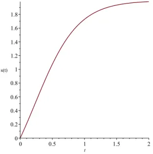
s(t) = 2e
3g(t)−2
e3g(t)+2 , t ≥0. (4.3)
Keeping the engine on at every time corresponds to the derivator g(t) = t for all t ≥ 0.
The corresponding solution is displayed in Figure4.1.
Figure 4.1: Solution (4.3) forg(t) =t (engine constantly on).
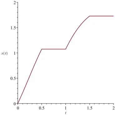
If we turn the device off fort∈[1/2, 1]∪[3/2, 2], then we should take
g(t) =
t, fort ∈[0, 1/2], 1/2, fort ∈[1/2, 1], t−1/2, fort ∈[1, 3/2], 3/2, fort ∈[3/2, 2].
The graph ofgand the solution given by (4.3) can be seen in Figures4.2and4.3, respectively.
Figure 4.2: Graph ofg(t).
Figure 4.3: Solution (4.3) with dead times (engine off).
4.2 Semicontinuous culture systems
Semicontinuous cultivation is a system to produce bacteria in which a portion of the culture medium is periodically removed and the remaining culture is used as the starting point for continuation of the culture. For the model in this section we take into account [5], where semicontinuous cultivation of the cyanobacteria Spirulina plantensisis studied. We highlight the following important feature of the system in [5]: illumination was controlled to have a 12 hours light/dark photoperiod, which resulted in two different reproduction phases every day.
Bearing the above considerations in mind, we shall set up a mathematical model for the production ofSpirulina plantensisin a semicontinuous culture system. First, we consider days as our time units. We assign light periods to be the time intervals [k,k+1/2),k = 0, 1, 2, . . . , while dark periods are [k+1/2,k+1), k = 0, 1, 2, . . . . Second, we assume that half of the culture is removed every 10 days and immediately refilled with new nutrients so that the remaining bacteria start reproducing again. Finally, we take as derivator a nondecreasing function g: [0,∞)→ [0,∞), continuous everywhere with the exception of the positive multi- ples of 10, and such that
g0(t) =
(1, if t∈(k,k+1/2),k =0, 1, 2, . . . , 1/2, if t∈(k+1/2,k+1),k =0, 1, 2, . . . ,
and g((10k)+)−g(10k) = 1 for k = 1, 2, 3, . . . A concise explicit expression for g(t) can be obtained by defining first its values on the first day, namely
h(t) =
(t, ift ∈[0, 1/2), t/2+1/4, ift ∈(1/2, 1],
and then we can define the remaining values by “periodicity”, and introducing jump discon-
tinuities at relevant places, as
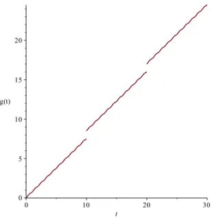
g(t) =h(t−[t]) +3[t]/4+ [t/10],
where [·] stands for the floor function. Observe that we should modify the values g(10k) (k = 1, 2, . . . ) so that g be left-continuous, but we shall not do it to avoid technicalities. See Figure4.4 for a plot of this function.
Figure 4.4: Graph of g(t) for a semicontinuous bacteria culture. Observe dif- ferent slopes for light and dark periods, and discontinuities at the renewal mo- ments.
We are now ready to introduce ag-differential model for the biomass concentrationx(t), measured in grams per liter at timet, with a given initial concentrationx(0) = x0. Biomass concentration should satisfy
x0g(t) = f(t,x(t)) t ≥0, x(0) =x0, (4.4) where f(t,x)is assumed to be logistic except at the renewal moments (positive multiples of 10), when we remove half of the culture and immediately refill the flask with new nutrients.
Specifically, we define
f(t,x) = (
αx(N−x), ift 6=10k,k =1, 2, . . . ,
−x/2, ift =10k,k=1, 2, . . . ,
whereα>0 and N>0 are biological parameters to be adjusted from experimental results.
Using the formulas (3.10) and (3.15), we compute the solution: fort∈[0, 10]the solution is
x(t) =
x0N
N−x0eαNg(t) 1+ x0
N−x0eαNg(t) .
Assume we have computedx(t)for allt∈ [0, 10k], for somek =1, 2, . . . , then we define xk =x(10k+) = x(10k)
2 , and the solution fort∈ (10k, 10k+10]is given by
x(t) =
xkN
N−xkeαN[g(t)−g(10k+)]
1+ xk
N−xkeαN[g(t)−g(10k+)]
.
Observe that g(10k+) =8.5k for allk=1, 2, . . .
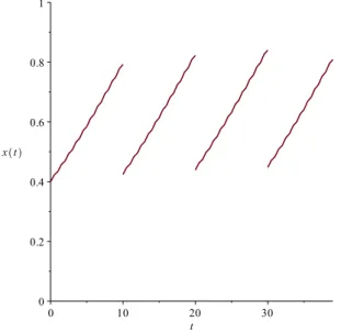
See Figure4.5 for a plot of the solution corresponding tox0= 0.4 grams per liter,α=0.1 and N= 1.5. These choices yield a good approximation of the experimental results obtained in [5] for the cyanobacteriaSpirulina platensis, see [5, Figure 2].
Figure 4.5: Biomassx(t)grams per liter in a semicontinuous culture, with initial density of 0.4 g/L, and parameters α=0.1,N =1.5.
5 Stieltjes equations with continuous derivators are just ODEs
The careful reader might have noticed that the solutions obtained for the previous examples are just the solutions of the corresponding ODEs, composed with the derivator g. In this section we will show that, under the assumption of continuity there is an equivalence between Stieltjes differential equations and ODEs.
It is pretty straightforward that a Stieltjes differential equation reduces to an ODE when the derivator is not only continuous, but also differentiable. Indeed, assume thatg∈ C1([t0,t0+T]). Then, for any t ∈ [t0,t0+T]\(Cg∪Ng)and anyx :[t0,t0+T]→ Rsuch that x0g(t)exists, it follows directly from the definition that x0(t)exists and
x0(t) =x0g(t)g0(t).
Therefore, ifxsolves (1.1) on[t0,t0+T]\(Cg∪Ng)then xsolves
x0(t) = f(t,x(t))g0(t), t∈ [t0,t0+T]\(Cg∪Ng). (5.1) More than that is true: since g0(t) = 0 for all t ∈ Cg∪Ng, the ODE (5.1) is satisfied on the whole interval I = [t0,t0+T].
Conversely, letc∈ L1([t0,t0+T]), c≥0, and assume thatx solves
x0(t) = f(t,x(t))c(t), t ∈ I = [t0,t0+T]. (5.2) Thenxsolves (1.1) on[t0,t0+T]\Nwith
g(t) =
Z t
t0 c(s)ds, t∈[t0,t0+T], andN={t ∈ I : c(t) =0}.
In what follows, we will show that we can still transform a Stieltjes differential equation into an ODE when we change the hypothesis of differentiability for just continuity.
Consider equation (1.1) with g : R → R nondecreasing and continuous, i.e., Dg = ∅.
Without loss of generality, we assume that g(R) =R (if not, it suffices to redefine g linearly outside the intervalI = [t0,t0+T], which has no influence on the equation).
We define the pseudo-inverse ofgas the functionγ:R→Rsuch that
γ(x) =min{t ∈R : g(t) =x} for each x∈R. (5.3) This definition is good. To prove it, just notice that g is continuous, nondecreasing and g(±∞) =±∞, which implies that
g−1({x}) ={t∈R : g(t) =x} (5.4) is a compact interval (even a singleton ifx 6∈Cg∪Ng).
The most important properties ofγare gathered in the following statement.
Proposition 5.1. Assume that g:R→Ris nondecreasing, continuous and g(R) =R. Ifγ:R→Ris defined as in(5.3), then the following properties hold:
1. for all x∈R, g(γ(x)) =x;
2. for all t∈R,γ(g(t))≤t;
3. for all t∈R, t6∈Cg∪Ng+,γ(g(t)) =t;
4. γis strictly increasing: x <y impliesγ(x)<γ(y);
5. γis left-continuous everywhere and continuous at every x∈R, x6∈g(Cg).
Proof. Property 1 is a direct consequence of the definition (5.3): g(γ(x))) = g(min{t : g(t) = x}) = x. For 2 observe thatγ(g(t)) = min{s : g(s) = g(t)} ≤ t. To prove 3 just note that t6∈Cg∪Ngimplies that the set (5.4) forx= g(t)is the singleton{t}. Now, ift ∈Ng−, we have that t = an0 for somen0 ∈ N. In that case, it is clear that g(t) = g(s) for alls ∈ (t,bn0)and g(s)< g(t)for alls< t, as any other case would lead to a contradiction. Thus, we have that
γ(g(t)) =min{s ∈R:g(t) =g(s)}=min(an0,bn0) =an0 =t.
For 4 we fix x < y and we note that if t ∈ g−1({x}) and s ∈ g−1({y}), then t < s, for otherwise we would havex =g(t)≥ g(s) =y, a contradiction. Henceγ(x) =ming−1({x})<
ming−1({y}) =γ(y).
Finally, we prove 5. First, property 4 ensures that
γ(x−)≤γ(x)≤γ(x+) for allx ∈R. (5.5) Assume, reasoning by contradiction, thatγ(x−)< γ(x)for some x. Sinceγis increasing, we can fixτsuch that
γ(y)<τ<γ(x) for ally< x. (5.6) Now we deduce from the monotonicity of gand property 1 that
y =g(γ(y))≤ g(τ)≤g(γ(x)) =x for ally <x,
which implies thatg(τ) =x. Now property 2 yieldsγ(x) =γ(g(τ))≤τ, a contradiction with (5.6). Henceγis left-continuous everywhere.
We shall prove thatγ is right-continuous at every x ∈ R\g(Cg)from (5.5) and a similar contradiction argument. Assume that for one of thosexwe can findτsuch that
γ(x)<τ<γ(y) for ally> x.
Since gis nondecreasing we have
x= g(γ(x))≤ g(τ)≤ g(γ(y)) =y for ally >x,
and thereforex= g(γ(x)) =g(τ). Sinceγ(x)<τ, for anyt∈(γ(x),τ)we haveg(t) =xand t∈Cg, a contradiction with the choice ofx.
We now have the necessary tools to reduce a Stieltjes differential equation to an ODE. First, we show how to compute solutions of Stieltjes equations by solving related ODEs.
Theorem 5.2. Assume that g:R→Ris nondecreasing, continuous and g(R) =R.
If y:[g(t0),g(t0+T)]→Ris a solution of
y0(s) = f(γ(s),y(s)), s∈ [g(t0),g(t0+T)]\C, (5.7) for some set C, then x:[t0,t0+T]→Rgiven by x(t) =y(g(t))solves(1.1)for all t∈ [t0,t0+T]\ (g−1(C)∪Cg∪Ng).
In particular, x= y◦g solves(1.1) g-almost everywhere in[t0,t0+T]provided that g−1(C)be a null g-measure subset of[t0,t0+T].
Proof. Fixt ∈ [t0,t0+T]\(g−1(C)∪Cg∪Ng). Then assertion 2 in Proposition5.1 yields that γ(g(t)) =tand, moreoverg(t)∈[g(t0),g(t0+T)]\C. Hencey0(g(t))exists and
y0(g(t)) = f(γ(g(t)),y(g(t))) = f(t,x(t)). Thus, it is enough to show thatx0g(t)exists and equalsy0(g(t)).
Fixε>0. Sincey0(g(t))exists, there exists ˜δ>0 such that z ∈[g(t0),g(t0+T)], 0<|z−g(t)|<δ˜
=⇒
y(z)−y(g(t))
z−g(t) −y0(g(t))
<ε.
On the other hand, sincegis continuous att, there existsδ>0 such that [s∈ [t0,t0+T], |s−t|<δ] =⇒ |g(s)−g(t)|<δ.˜
Now, Remark2.1 ensures that if 0< |s−t| < δ then 0< |g(s)−g(t)|< δ. Hence, it follows˜ that
[s∈ [t0,t0+T], 0< |s−t|<δ] =⇒
y(g(s))−y(g(t))
g(s)−g(t) −y0(g(t))
<ε, that is,x0g(t)exists andx0g(t) =y0(g(t)).
Example 5.3. We consider problem (4.1) again, fors0=0 and f(s) = [(s+1)(2−s)]+.
Assuming a derivatorgin the conditions of Theorem 5.2and g(0) = 0, we just have to solve the initial value problem
y0(s) = f(y(s)), y(0) =0, and then we get a solution of the Stieltjes problem (4.1) in the form
s(t) =y(g(t)) = 2e
3g(t)−2
e3g(t)+2 , t≥0.
Next we prove the converse result, thus showing that problems (1.1) and (5.7) are equiva- lent.
Theorem 5.4. Assume that g:R→Ris nondecreasing, continuous and g(R) =R.
If x:[t0,t0+T]→Ris a solution of (1.1)for all t∈ [t0,t0+T]\(C∪Cg∪Ng)for some set C, then y :[g(t0),g(t0+T)]→R given by y(t) = x(γ(t))solves(5.7) for all t∈ [g(t0),g(t0+T)]\ g(C∪Cg∪Ng).
In particular, y = x◦γsolves m-almost everywhere in [g(t0),g(t0+T)]provided that m−1(C) be a null m-measure subset of[g(t0),g(t0+T)].
Proof. Fixs∈[g(t0),g(t0+T)]\g(C∪Cg∪Ng). Then there existsu∈ [t0,t0+T]\C∪Cg∪Ng such that g(u) = s. Moreover, Remark 2.1 ensures that g−1({s}) = {u} so γ(s) = u ∈ [t0,t0+T]\C∪Cg∪Ng andx0g(γ(s))exists. Furthermore,
x0g(γ(s)) = f(γ(s),x(γ(s))) = f(γ(s),y(s)), so, it is enough to show thaty0(s)exists and equals x0g(γ(s)).
Fixε>0. Since x0g(γ(s))exists, there exists ˜δ>0 such that z∈ [t0,t0+T], 0< |z−γ(s)|<δ˜
=⇒
x(z)−x(γ(s))
g(z)−g(γ(s))−x0g(γ(s))
<ε.
On the other hand, s ∈ [g(t0),g(t0+T)]\g(C∪Cg∪Ng) so assertion 4 in Proposition 5.1 ensures thatγis continuous ats. Hence, there existsδ >0 such that
[r ∈[g(t0),g(t0+T)], |r−s|<δ] =⇒ |γ(r)−g(s)|<δ.˜
Now, assertion 3 in Proposition5.1guarantees that if 0<|s−t|<δthen 0 <|g(s)−g(t)|<δ.˜ Hence, it follows that
[r ∈[g(t0),g(t0+T)], 0<|r−s|< δ] =⇒
x(γ(r))−x(γ(s))
g(γ(r))−g(γ(s))−x0g(γ(s))
<ε.
The result now follows by property 1 in Proposition5.1.
Remark 5.5. It is possible to extend theorems5.2and5.4to problem (1.1) with f :I×Rn→Rn with the obvious changes.
As a final comment, note that the results in this section are not valid for discontinuous derivatorsg. However, ifDg is a discrete set, then we can argue “piece-by-piece” to obtain the general solution of (1.1). That is, we can use the results in this section to solve (5.7) in each of the subintervals generated by Dg.
Acknowledgements
Rodrigo López Pouso was partially supported by Ministerio de Economía y Competitivi- dad, Spain, and FEDER, Project MTM2016-75140-P and Xunta de Galicia under grant ED431C 2019/02. Ignacio Márquez Albés was supported by Xunta de Galicia under grants ED481A- 2017/095 and ED431C 2019/02.
References
[1] M. Frigon, R. LópezPouso, Theory and applications of first-order systems of Stieltjes differential equations, Adv. Nonlinear Anal. 6(2017), No. 1, 13–36. https://doi.org/10.
1515/anona-2015-0158
[2] R. LópezPouso, I. MárquezAlbés, General existence principles for Stieltjes differential equations with applications to mathematical biology, J. Differential Equations 264(2018), No. 8, 5388–5407.https://doi.org/10.1016/j.jde.2018.01.006
[3] R. LópezPouso, A. Rodríguez, A new unification of continuous, discrete, and impulsive calculus through Stieltjes derivatives,Real Anal. Exchange40(2014/15), No. 2, 1–35.https:
//doi.org/10.14321/realanalexch.40.2.0319
[4] G. A. Monteiro, B. Satco, Distributional, differential and integral problems: equivalence and existence results,Electron. J. Qual. Theory Differ. Equ.2017, No. 7, 1–26.https://doi.
org/10.14232/ejqtde.2017.1.7
[5] C. C. Reichert, C. O. Reinehr, J. A. V. Costa, Semicontinuous cultivation of the cyanobacterium Spirulina platensis in a closed photobioreactor, Braz. J. Chem. Eng.
23(2006), 23–28.https://doi.org/10.1590/S0104-66322006000100003