DELAY DIFFERENTIAL EQUATIONS IN BIOMATHEMATICS
PhD Thesis By
Nahed Abdelfattah Mohamady Abdelfattah
Supervisors: Professor Istv´an Gy˝ori Professor Ferenc Hartung
UNIVERSITY OF PANNONIA
Doctoral School of Information Science and Technology University of Pannonia
Veszpr´em, Hungary 2017
DOI:10.18136/PE.2017.648
Thesis for obtaining a PhD degree in
the Doctoral School of Information Science and Technology of the University of Pannonia.
Written by:
Nahed Abdelfattah Mohamady Abdelfattah
Written in the Doctoral School of Information Science and Technology of the Univer- sity of Pannonia.
Supervisors: Prof. Istv´an Gy˝ori and Prof. Ferenc Hartung propose acceptance (yes / no) propose acceptance (yes / no)
(signature) (signature)
The candidate has achieved ... % in the comprehensive exam, Veszpr´em,
...
Chairman of the Examination Committee As reviewer, I propose acceptance of the thesis:
Name of reviewer: ... ( yes / no)
...
(signature) Name of reviewer: ... ( yes / no)
...
(signature) The candidate has achieved ... % at the public discussion.
Veszpr´em,
...
Chairman of the Committee Grade of the PhD diploma ...
...
President of UCDH
First of all, All gratitude and thankfulness to ALLAH for guiding and aiding me to bring this work out to light. Also, it is impossible to give sufficient thanks to the people who gave help and advice during the writing of this thesis. However, I would like to single out both of my supervisors Prof. Istv´an Gy˝ori and Prof. Ferenc Hartung for their guidance, their valuable discussions and enriching collaborations throughout my years as a PhD student in Hungary. Without their kind help, gen- erous encouragement and their vital comments on the contents of this thesis, this work would not have seen the light.
I would like to thank the Director of the Doctoral School (Prof. Katalin Hangos) for her help and support, also I have the pleasure to thank everyone in Department of Mathematics and everybody helped me in Hungary.
I would like to thank the reviewers for my home defence (Dr. Tam´as Insperger and Dr. R¨ost Gergely) for their valuable comments and suggestions that helped to improve my Thesis.
Many thanks for all my friends and colleagues in Veszpr´em, they played a very important role in my life.
The last, but the most important thanks to my family: my father, my mother, my husband and my daughters for their love, also for keeping me in their prayers.
iii
A dolgozatban nemline´aris k´esleltetett argumentum´u skal´aris differenci´alegyenletek illetve differenci´alegyenlet-rendszerek egy sz´eles oszt´aly´at vizsg´aljuk. Az ilyen egyen- letek gyakran megjelennek term´eszettudom´anyi, k¨ozgazdas´agtani, m´ern¨oki, popul´a- ci´odinamikai, epidemiol´ogiai alkalmaz´asokban. Mivel az ´altalunk tekintett model- leket popul´aci´odinamikai alkalmaz´asok motiv´alt´ak, pozit´ıv megold´asokra f´okusz´a- lunk, ´es a modellek pozit´ıv megold´asai perzisztenci´aj´at ´es egyenletes permanenci´aj´at vizsg´aljuk. A f˝o eredm´enyeink alkalmaz´asak´ent explicit becsl´eseket fogalmazunk meg a megold´asok limesz inferiorj´ara ´es limesz szuperiorj´ara. Egyszer˝u skal´aris mo- dellek eset´en visszakapjuk az irodalomb´ol ismert becsl´eseket, de gyeng´ebb felt´etelek mellett. A bizony´ıt´asaink ¨osszehasonl´ıt´o t´eteleken ´es a monoton iter´aci´os technik´an alapulnak. Rendszerek eset´eben a becsl´eseinkhez meg kell oldani egy kapcsol´o- d´o nemline´aris algebrai egyenletrendszert. Elegend˝o felt´eteleket adunk meg ilyen egyenletrendszer megold´asai l´etez´es´ere ´es egy´ertelm˝us´eg´ere. Az eredm´enyeink is- mert eredm´enyeket terjesztenek ki l´enyegesen ´altal´anosabb egyenletoszt´alyokra, ´es a haszn´alt felt´eteleink gyeng´ebbek az irodalomban eddig vizsg´alt esetekhez k´epest.
Elegend˝o felt´eteleket adunk meg bizonyos egyenletek eset´eben a megold´asok aszimp- totikus ekvivalenci´aj´ara. Az ´uj eredm´enyeket sz´amos p´elda ´es numerikus szimul´aci´o illusztr´alja.
iv
In this work, we study a large family of scalar differential equations and systems of differential equations with delays. Such equations appear frequently as mathemat- ical models in natural sciences, economics and engineering, population dynamics, mathematical epidemiology and other engineering applications. Since our model equations are motivated by applications in population dynamics, we focus only on positive solutions, and we investigate persistence and permanence of the positive solutions of our model equations. As an application of the main results, we obtain explicit estimates for the limit inferior and limit superior of the solutions. For some simple scalar population models, our method recovers known estimates of the lit- erature, but under weaker conditions. Our method uses comparison technique and iterative methods of differential equations. For the system case, our results requires the solutions of an associated system of nonlinear algebraic equations. We establish sufficient conditions implying the existence and uniqueness of solutions of such sys- tem of algebraic equations. These results generalize known methods for much larger classes of equations, and our conditions are weaker for the previously studied cases too. For a special class of differential equations, we give sufficient conditions for the asymptotic equivalence of the positive solutions. All the new results are illustrated by several special examples and numerical experiments too.
v
Acknowledgments iii
Tartalmi kivonat iv
Abstract v
List of Figures viii
List of Tables ix
1 Introduction 1
1.1 Background and motivation . . . 1 1.2 The structure and content of the Thesis . . . 4 1.3 Notations . . . 5
2 Theoretical Background 7
2.1 Scalar delay differential equations . . . 7 2.2 Mathematical and biological models . . . 9 2.3 Numerical approximation of delay equations . . . 11 3 On a nonlinear scalar delay population model 14 3.1 Introduction and preliminaries . . . 15 3.2 Main results of Chapter 3 . . . 16
vi
3.3 Applications of the main results . . . 23
3.4 Examples . . . 35
4 Existence and uniqueness of solutions of algebraic systems 42 4.1 Introduction . . . 42
4.2 Main results of Chapter 4 . . . 46
4.3 Applications . . . 51
4.3.1 Nonlinear systems . . . 51
4.3.2 Two dimensional systems . . . 55
5 Boundedness of positive solutions of a system of DDEs 59 5.1 Introduction . . . 60
5.2 Main Results of Chapter 5 . . . 63
5.3 Corollaries . . . 72
5.4 Applications to some population models . . . 75
5.5 Examples . . . 81
6 Conclusion 90 6.1 New scientific results . . . 90
6.2 Publications and conference lectures . . . 92
6.2.1 Publications in refereed SCI journal (related to this Thesis) . 93 6.2.2 Publication in refereed journal (not related to this Thesis) . . 93
6.2.3 International conference presentations related to the Thesis . . 94
Bibliography 95 Appendix A 103 A.1 Proofs of some results in Chapter 3 . . . 103
A.2 Proofs of some results in Chapter 5 . . . 105
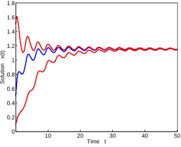
3.4.1 Solutions of Eq. (3.4.1) corresponding to the initial functions ϕ(t) =
0.2, ϕ(t) = 1 and ϕ(t) = 2 . . . 36
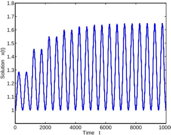
3.4.2 Solution of Eq. (3.4.2) corresponding to the initial function ϕ(t) = 1 and τ = 1000 . . . 37
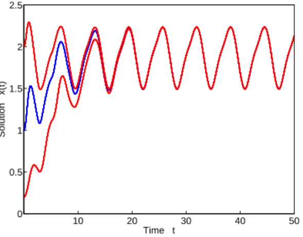
3.4.3 Solution of Eq. (3.4.3) corresponding to the initial functions ϕ(t) = 0.5, ϕ(t) = 1.1 and ϕ(t) = 2.8 . . . 38
3.4.4 Solutions of Eq. (3.4.4) corresponding toδ = 0.8 and the initial func- tions ϕ(t) = 0.1,ϕ(t) = 0.5 and ϕ(t) = 1.5. . . 39
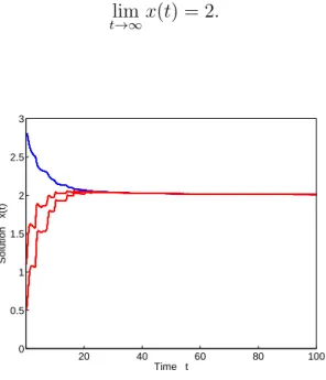
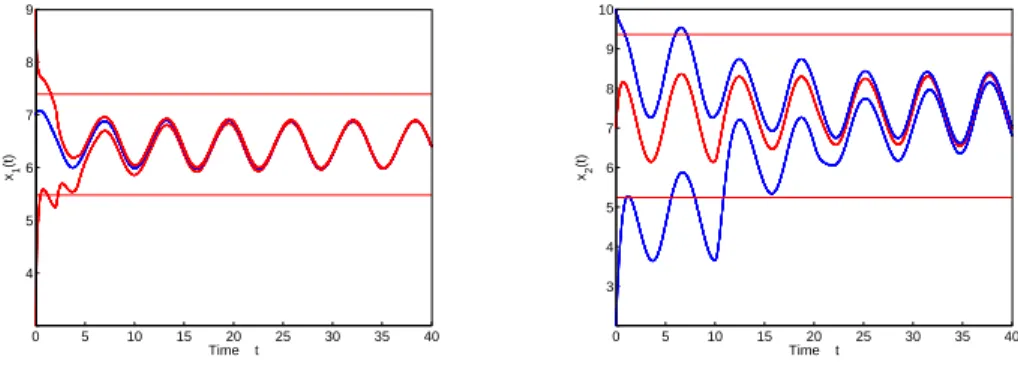
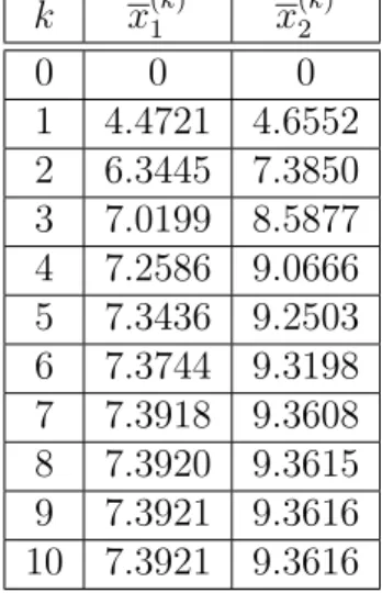
3.4.5 Solution of Eq. (3.4.5) corresponding to the initial functions ϕ(t) = 1 40 5.5.1 Numerical solution of the System (5.5.1). . . 83
5.5.2 Numerical solution of the System (5.5.6). . . 85
5.5.3 Numerical solution of the System (5.5.11). . . 87
5.5.4 Numerical solution of the System (5.5.16). . . 89
viii
5.5.1 Numerical solution of the System (5.5.2) . . . 83
5.5.2 Numerical solution of the System (5.5.4) . . . 83
5.5.3 Numerical solution of the System (5.5.7) . . . 86
5.5.4 Numerical solution of the System (5.5.9) . . . 86
5.5.5 Numerical solution of the System (5.5.12) . . . 87
5.5.6 Numerical solution of the System (5.5.14) . . . 87
5.5.7 Numerical solution of the System (5.5.17) . . . 89
ix
Introduction
In modelling in the biological, physical and social sciences, it is sometimes necessary to take account of time delays inherent in the phenomena. In all these fields scientists need their models to behave more like the real process. Many processes include aftereffect phenomena in their inner dynamics. In these cases, it may be necessary to choose between a model with discrete delays or a model with distributed delay.
1.1 Background and motivation
Time delays of one type or another have been incorporated into biological models to represent resource regeneration times, maturation periods, feeding times, reaction times, etc. by many researchers. We refer to the monographs of ([26], [27], [35], [57], [60]) for discussions of general delayed biological systems. In general, delay differen- tial equations exhibit much more complicated dynamics than ordinary differential equations since a time delay could cause a stable equilibrium to become unstable and cause the populations to fluctuate. In this section, we shall review various delay differential equations models arising from studying single species dynamics. Letx(t) denote the population size at time t; let b and d denote the birth rate and death
1
rate, respectively, on the time interval [t, t+ ∆t], where ∆t >0. Then x(t+ ∆t)−x(t) =bx(t)∆t−dx(t)∆t.
Dividing by ∆t and letting ∆t approach zero, we obtain dx
dt =bx−dx=rx, (1.1.1)
where r = b− d is the intrinsic growth rate of the population. The solution of equation (1.1.1) with an initial population x(0) =x0 is given by
x(t) = x0ert. (1.1.2)
The function (1.1.2) represents the traditional exponential growth if r > 0 or decay if r < 0 of a population. Such a population growth, due to Malthus (1798), may be valid for a short period, but it cannot go on forever. Verhulst (1836) proposed the logistic equation
dx
dt =rx 1− x
K
, (1.1.3)
where r > 0 is the intrinsic growth rate and K > 0 is the carrying capacity of the population. In model (1.1.3), when x is small the population grows as in the Malthusian model (1.1.1); when xis large the members of the species compete with each other for the limited resources. Solving (1.1.3) by separating the variables, we obtain (x(0) =x0),
x(t) = x0K
x0−(x0−K)e−rt. (1.1.4) If 0 < x0 < K, the population grows, approaching K asymptotically as t → ∞. If x0 > K, the population decreases, again approaching K asymptotically as t→ ∞.
If x0 = K, the population remains in time at x = K. In fact, x = K is called the equilibrium of equation (1.1.3). Thus, the positive equilibrium x = K of the logistic equation (1.1.3) attracts all the positive solutions; that is, lim
t→∞x(t) =K, for solutionx(t) of (1.1.3) with any positive initial valuex(0) =x0.
In the above logistic model it is assumed that the growth rate of a population at any time t depends on the relative number of individuals at that time. In practice, the process of reproduction is not instantaneous. For example, in a Daphnia a large clutch presumably is determined not by the concentration of unconsumed food available when the eggs hatch, but by the amount of food available when the eggs were forming, some time before they pass into the broad pouch. Between this time of determination and the time of hatching many newly hatched animals may have been liberated from the brood pouches of other Daphnia in the culture, so increasing the population. Hutchinson [52] assumed egg formation to occur τ units of time before hatching and proposed the following more realistic logistic equation
dx(t)
dt =rx(t)
1−x(t−τ) K
, (1.1.5)
where r and K have the same meaning as in the logistic equation (1.1.3), τ > 0 is a constant. Equation (1.1.5) is often referred to as the Hutchinson’s equation or delayed logistic equation and was introduced with the initial condition
x(t) = ϕ(t), −τ ≤t≤0, (1.1.6)
where, ϕis continuous on [−τ,0].
In this Thesis we focus on the study of boundedness of the positive solutions of differential equations with time delays, that appear frequently as mathematical models in natural sciences, economics and engineering, population dynamics, math- ematical epidemiology, economics and large classes of engineering applications and many others. Since our model equations are motivated by applications in population dynamics, we focus only on positive solutions, and we investigate persistence and permanence of the positive solutions.
1.2 The structure and content of the Thesis
The structure of the Thesis is the following. In Chapter 1 we give a list of notations we use in the rest of the Thesis.
In Chapter 2 we give some basic background, known results and notions on the topics we will use in later chapters in our investigation.
In Chapter 3 we study the persistence and the uniform permanence of the positive solutions of the general nonlinear scalar delay differential equation
˙
x(t) = r(t)
g(t, xt)−h(x(t))
, t≥0,
and present sufficient conditions which guarantee the boundedness of the solution (see Theorem 3.2.4 ). This general form of the equation may include a single or multiple constant or time-dependent point delay functions as well as distributed delays in the positive terms. Corollary 3.3.1 immediately implies the estimates obtained in [4], but under weaker conditions. Our method is based on the well- known comparison theorem for differential equations. We give also, in Section 3.3, several particular cases and explicit estimations for the upper and lower limit of the solutions. We investigated in some special cases conditions, which imply that all solutions have the same asymptotic behavior, i.e., the difference of any two positive solutions tends to zero.
In Chapter 4 we give sufficient conditions which imply the existence and unique- ness of the positive solutions of the general nonlinear system of algebraic equations
γi(xi) =
n
X
j=1
gij(xj), 1≤i≤n.
Our main result, Theorem 4.2.1 below, uses a monotone iterative method to prove existence of a positive solution, and an the extension of the method used in [21] to prove uniqueness under a weaker condition than that assumed in [21]. We introduce many applications and special cases of our main results and in some cases we give
necessary conditions for the existence and uniqueness of the positive solutions. Also we give a counterexample which shows the importance of our conditions.
In Chapter 5 we consider the system of nonlinear delay differential equations
˙ xi(t) =
n
X
j=1 n0
X
`=1
αij`(t)hij(xj(t−τij`(t)))−ri(t)fi(xi(t)) +ρi(t), t≥0, 1≤i≤n, and give sufficient conditions for the uniform permanence of the positive solutions of the system. Also in several particular cases, explicit estimates are given for the upper and lower limit of the solutions.
In Chapter 6 we summarize the new results. Also the list of publications and conference lectures of Nahed A. Mohamady related to the topic of this Thesis is given.
In Appendix A we present some technical or long proofs.
1.3 Notations
The most important notations used throughout in this Thesis are listed below in this section.
Mathematical notations
R the set of real numbers
R+ := [0,∞) the set of non-negative real numbers
C(X, Y) the set of continuous functions mapping from X toY C the set of continuous functions mapping from [−τ,0] to R
C+ the set of continuous functions mapping ψ from [−τ,0] to R+ with ψ(0)>0 C0 the set of continuous functions mapping ψ from [−τ,0] to R+ with ψ(t)>0,
−τ ≤t≤0
k · kτ the maximum norm of a continuous function x: [−τ,0]→Rn defined by kxkτ := max
−τ≤t≤0kx(t)k
xt(θ) the segment function defined by xt(θ) := x(t+θ), θ∈[−τ,0], where x is a function defined from [−τ,∞) to R, and t ∈R+
˙
x= dxdt time derivative ofx x(∞) := lim inf
t→∞ x(t)
x(∞) := lim sup
t→∞
x(t)
xi ith element of a vector x xT transpose of a vector x.
Next we list the acronyms we use in the Thesis.
Acronyms
IVP initial value problem
ODEs ordinary differential equations DDEs delay differential equations Eq equation.
Theoretical Background
In this chapter we review some concepts and known results which are used or referred to later in the Thesis.
2.1 Scalar delay differential equations
In this section we investigate a scalar delay differential equation which will be useful in the rest of the Thesis.
Consider the scalar nonlinear differential equation with general delays
˙
x(t) =f(t, xt), t≥t0, (2.1.1)
and the initial condition
x(t) =ϕ(t−t0), t0−τ ≤t≤t0, (2.1.2) where τ > 0, t0 ≥0, ϕ∈ C :=C([−τ,0],R), f : [t0,∞)×C →R is continuous and xt(θ) :=x(t+θ), θ ∈[−τ,0].
Definition 2.1.1. A function x is called a solution of Eq. (2.1.1) on [t0 −τ,∞) if x ∈ C([t0−τ,∞),R), (2.1.2) holds and x satisfies Eq. (2.1.1) for t ∈[t0, β) for some β > t0 or for t∈[t0,∞).
Definition 2.1.2. A function f : [t0,∞)×C → R is called locally Lipschitz in its 7
second variable, if for any t ∈ [t0,∞) and ϕ ∈ C, there exist δ1 > 0, δ2 > 0 and L >0 constants such that
kf(s, ψ1)−f(s, ψ2)k ≤Lkψ1−ψ2kτ,
fors ∈[t−δ1, t+δ1]andψ1, ψ2 ∈C satisfyingkψ1−ϕkτ ≤δ2 and kψ2−ϕkτ ≤δ2, where kψkτ := max
−τ≤s≤0kψ(s)k.
We recall, from [30], the following theorem of the existence and uniqueness of solution of the IVP (2.1.1) and (2.1.2).
Theorem 2.1.1. [30] Let f : R+ ×C → R be continuous and locally Lipschitz continuous in its second variable. Then, for every t0 ≥ 0 and ϕ ∈ C, there exists β > t0 such that the IVP (2.1.1) and (2.1.2) has a unique solution on [t0−τ, β).
We note that this result can be naturally extended to systems of delay differential equations too.
The following comparison theorem of differential equations will be essential in our proofs later.
Theorem 2.1.2. Let f :R+×C →R and g :R+×R→ R be continuous, φ∈ C, and t0 ≥0 be fixed. Let x be a solution of the IVP
˙
x(t) = f(t, xt), t≥t0, (2.1.3)
x(t) = ϕ(t−t0), t ∈[t0−τ, t0], (2.1.4) and let y be a unique solution of the IVP
˙
y(t) =g(t, y(t)), t ≥t0, (2.1.5)
y(t0) = ϕ(0). (2.1.6)
Then if f(t, ψ) ≥ g(t, ψ(0)), for all (t, ψ) ∈ R+×C, there follows x(t) ≥ y(t) for t≥t0. Also, iff(t, ψ)≤g(t, ψ(0)), for all (t, ψ)∈R+×C, there follows x(t)≤y(t) for t≥t0.
Proof. The proof is given in [15] for the case when (2.1.3) is an ODE, but it
can be easily extended to this case too.
The notions of persistence and permanence are frequently studied in mathemat- ical biology (see e.g. [57, 60]). Following [3, 4, 31] and [33] we define the next two notions. Let us, first, define the classC+ :={ψ ∈C([−τ,0],R+) : ψ(0) >0}, where τ >0.
Definition 2.1.3. Eq. (2.1.1) is said to be persistent in C+ if any positive solution x(t) is bounded away from zero, i.e., lim inf
t→∞ x(t)>0.
Definition 2.1.4. Eq. (2.1.1) is called uniformly permanent if there exist two pos- itive numbers m and M with m < M such that, all positive solutions x(t) of Eq. (2.1.1) satisfy
m≤lim inf
t→∞ x(t)≤lim sup
t→∞
x(t)≤M.
2.2 Mathematical and biological models
In this section, we look at some ways mathematics is used to model dynamic pro- cesses in biology. Interactions between the mathematical and biological sciences have been appearing rapidly in recent years. Both traditional topics, such as population and disease modeling, and new ones, have made biomathematics an exciting field.
Simple formulas relate, for instance, the population of a species in a certain year to that of the following year. We consider the biological models as nonlinear delay differential equations. Although many of the models we examine may at first seem to be gross simplifications, their very simplicity is a strength. Simple models show clearly the implications of our most basic assumptions. We begin by considering the scalar nonautonomous differential equation
N˙(t) =a(t)N(t)−r(t)N2(t), t≥0 (2.2.1)
which is known as the logistic equation in mathematical ecology. Eq. (2.2.1) is a pro- totype in modeling the dynamics of single species population systems whose biomass or density is denoted by a function N of the time variable. The functionsa(t) and r(t) are time dependent net birth and self-inhibition rate functions, respectively.
The carrying capacity of the habitat is the time dependent function K(t) = a(t)
r(t), t≥0. (2.2.2)
By using this notation, Eq. (2.2.1) can be written as N˙(t) = r(t)
K(t)N(t)−N2(t)
, t≥0, (2.2.3)
or
N˙(t) =r(t)
K0N(t)−N2(t)
, t≥0 (2.2.4)
whenever the carrying capacity is constant, i.e., K(t) = K0,t ≥0 with a K0 >0.
It follows by elementary techniques that the above equations with the initial condition
N(0) =N0 >0 (2.2.5)
has a unique solutionN(N0)(t) of the initial value problem (IVP) (2.2.4) and (2.2.5) given by the explicit formula
N(N0)(t) = N0K0eK0R0tr(s)ds
K0+N0(eK0R0tr(s)ds −1), t≥0. (2.2.6) From the above formula, we get that either
Z ∞ 0
r(s)ds =∞ (2.2.7)
and
N(N0)(∞) := lim
t→∞N(t) = K0 for any N0 >0, or
Z ∞ 0
r(s)ds <∞ (2.2.8)
and
N(N0)(∞) = N0K0eK0R0∞r(s)ds
K0+N0(eK0R0∞r(s)ds−1) 6=K0 for any N0 6=K0.
ThusK0 is a global attractor of (2.2.4) with respect to the positive solutions if and only (2.2.7) holds.
It follows by some elementary technique that for any N0 > 0 the solution N(N0)(t) of the IVP (2.2.3) and (2.2.5) obeys
K(∞)≤lim inf
t→∞ N(N0)(t)≤lim sup
t→∞
N(N0)(t)≤K(∞) (2.2.9) for any N0 >0, if
0< K(∞) := lim inf
t→∞ K(t)≤lim sup
t→∞
K(t) =:K(∞)<∞ (2.2.10) and (2.2.7) holds.
In (1948) Hutchinson [52] considered the delayed logistic equation N˙(t) =rN(t)
1− N(t−τ) K0
, (2.2.11)
where r =b−d is the intrinsic growth rate of the population and K0 >0 has the same meaning as in the logistic equation (2.2.4), τ > 0 is a constant. Equation (2.2.11) was introduced with the initial condition
N(t) = ϕ(t), −τ ≤t≤0, (2.2.12)
where, ϕ is continuous on [−τ,0]. It is interesting to note that Equation (2.2.11) can be observed in some Daphnia populations. We refer the reader to ([25, 35, 47, 48, 57, 64, 65, 66, 72]) who have argued that the delay should enter in the birth term rather than in death term.
2.3 Numerical approximation of delay equations
In this section, we investigate numerical approximation of differential equations using the class of delay differential equations with piecewise constant arguments.
Equations with piecewise constant arguments were introduced by Wiener [68] and
Cooke and Wiener [22, 23]. For surveys of theory and applications of such equations we refer to [1, 24, 69]. We present a numerical approximation method which was introduced first for linear delay equations in [40], and later it was extended for various classes of differential equations (see [43]).
We introduce the method for nonlinear delay equations of the form
˙
x(t) =f(t, x(t), x(t−τ)), t ≥0, (2.3.1) with initial condition
x(t) = ϕ(t), −τ ≤t≤0. (2.3.2)
Let h > 0 be a discretization parameter. We associate the following equation with piecewise constant arguments to the IVP (2.3.1)-(2.3.2)
˙
yh(t) = f([t/h]h, yh([t/h]h), yh([t/h]h−[τ /h]h)), t ≥0 (2.3.3) and
yh(t) = ϕ(t), −τ ≤t ≤0, (2.3.4)
where [·] denotes the greatest integer part function.
Following [40] we have the following definition for the solution of the IVP (2.3.3)- (2.3.4):
Definition 2.3.1. By a solution of the IVP (2.3.3)-(2.3.4), we mean a function yh defined on {−kh : k ∈ N,−τ ≤ −kh ≤ 0} by (2.3.4), which satisfies the following properties on R+:
(i) the function yh is continuous on R+,
(ii) the derivativey˙h exists for eacht∈R+ with the possible exception of the points kh(k= 0,1,2, ...) where finite one-sided derivative exist, and
(iii) the functionyh satisfies (2.3.3) on each interval[kh,(k+1)h)fork = 0,1,2, ....
The right-hand-side of (2.3.3) is constant on the intervals [kh,(k+ 1)h), so the solution of (2.3.3)-(2.3.4) is a continuous function which is linear in between the mesh points {kh:k ∈N}. Define `:= [τ /h].
We integrate both sides of (2.3.3) from kh tot, Z t
kh
˙
yh(s)ds= Z t
kh
f([s/h]h, yh([s/h]h), yh([s/h]h−`h))ds,
wherekh≤t <(k+1)h. Using that the integrand on the right-hand-side is constant, we get
yh(t)−yh(kh) =f(kh, yh(kh), yh(kh−`h))(t−kh).
Now taking the limit t →(k+ 1)h from the left-hand, we have yh((k+ 1)h)−yh(kh) = hf(kh, yh(kh), yh(kh−`h)).
Since yh is linear between the mesh points, the values a(k) = yh(kh) uniquely determine the solution. The sequence a(k) satisfies the difference equation
a(k+ 1) =a(k) +f(kh, a(k), a(k−`))·h, k= 0,1,2, . . . , a(−k) =ϕ(−kh), k = 0,1,2, . . . , −τ ≤kh≤0.
It was shown in [40, 43] that
h→0lim|x(t)−yh(t)|= 0, for all fixed t ≥0.
In all the numerical examples of this Thesis we will use the above numerical ap- proximation method. For other numerical methods to approximate delay equations we refer to [5].
On a nonlinear scalar delay population model
In this chapter we consider a nonlinear scalar delay differential equation and establish sufficient conditions for the uniform permanence of the positive solutions of the equation.
This chapter is organized as follows: Section 3.1 introduces a description of our nonlinear delay differential equation and some basic definitions and preliminaries.
Section 3.2 presents the main results of this chapter for the uniform permanence of the positive solutions of the equation. In Section 3.3, several particular cases are introduced and explicit formulas are given for the upper and lower limit of the solutions. Also, in some special cases, sufficient conditions, which imply that the difference of any two positive solutions tends to zero, are given. In Section 3.4, several examples with numerical simulations are given to illustrate the main results.
14
3.1 Introduction and preliminaries
In this chapter, we investigate lower and upper estimates for the positive solutions of the nonlinear scalar delay differential equation
˙
x(t) = r(t)
g(t, xt)−h(x(t))
, t≥0, (3.1.1)
where τ > 0 is fixed, xt(θ) = x(t +θ), −τ ≤ θ ≤ 0, r, h ∈ C(R+,R+), g ∈ C(R+ × C,R+). Eq. (3.1.1) can be considered as a population model equation with delay in the birth term r(t)g(t, xt), and no delay in the self-inhibition term r(t)h(x(t)). The form of the delay model is based on the works of the authors [12, 25, 35, 47, 48, 57, 64, 65, 66, 72]. Eq. (3.1.1) includes, e.g., the next equations
˙ x(t) =
n
X
k=1
αk(t)x(t−τk(t))−β(t)x2(t), t≥0, (3.1.2)
˙ x(t) =
n
X
k=1
αk(t)xp(t−τk(t))−β(t)xq(t), t ≥0, 0< p < q, q≥1, (3.1.3)
˙
x(t) =α(t)f(x(t−τ))−β(t)g(x(t)), t≥0, (3.1.4) and
˙
x(t) = α(t)x(t−τ)
1 +γ(t)x(t−τ) −β(t)x2(t), t ≥0 (3.1.5) with discrete delays, or
˙
x(t) = α(t) Z 0
−τ
f(s, x(t+s))ds−β(t)h(x(t)), t≥0 (3.1.6) with distributed delay.
Recently, lower and upper estimations of the positive solutions of Eq. (3.1.2) were proved in [4] and [31] under the assumptions that the coefficients αk and β satisfy
α0 ≤αk(t)≤A0, β0 ≤β(t)≤B0, t ≥0, k = 1, . . . , n (3.1.7) with some positive constants α0, A0, β0 and B0. The following theorem, which is a
consequence of our main results, illustrate that the above boundedness conditions can be released. In this statement we investigate the qualitative behavior of the solution of Eq. (3.1.2) under the initial condition
x(t) = ϕ(t), −τ ≤t≤0, (3.1.8)
whereϕ∈C+. The unique solution of Eq. (3.1.2) and (3.1.8) is denoted byx(ϕ)(t).
We will assume
αk, τk ∈C(R+,R+), (k = 1, . . . , n), τ := max
1≤k≤nsup
t≥0
τk(t)<∞, (3.1.9)
β ∈C(R+,(0,∞)),
Z ∞ 0
β(t)dt=∞, (3.1.10)
and
0< m:= lim inf
t→∞
1 β(t)
n
X
k=1
αk(t) and m:= lim sup
t→∞
1 β(t)
n
X
k=1
αk(t)<∞.
(3.1.11) We note that Eq. (3.1.2) has no constant positive steady-state if the function
1 β(t)
n
P
k=1
αk(t) is not constant.
Our proof is based on using some relevant well-known theorem for differential inequalities of ordinary differential equations, moreover we can apply our method for differential equations with distributed delay, e.g., of the form (3.1.6), where techniques of [4] and [31] do not work.
3.2 Main results of Chapter 3
Throughout this chapter we use the following notations.
x(∞) := lim inf
t→∞ x(t) and x(∞) := lim sup
t→∞
x(t).
We consider the scalar nonlinear delay equation
˙
x(t) = r(t)
g(t, xt)−h(x(t))
, t≥0, (3.2.1)
with the initial condition
x(t) = ϕ(t), −τ ≤t≤0. (3.2.2)
Next we list the following conditions, which will be used only whenever this is explicitly indicated:
(H1) r∈C(R+,R+) withr(t)>0 for t >0 andR∞
0 r(s)ds=∞,g ∈C(R+×C,R) with g(t, ψ)≥0 fort ≥0 and ψ(s)≥0, −τ ≤s≤0.
(H2) h∈C(R+,R+) satisfies 0 =h(0)< h(x1)< h(x2) for 0< x1 < x2,and for any nonnegative constants v and L satisfying L 6= v the condition Rv
L ds h(v)−h(s) = +∞holds.
(H3) There exists q1 ∈C(R2+,R+) such that for any T ≥0, u > 0 we have g(t, ψ)≥q1(T, u), if t≥T and ψ ∈C with ψ(s)≥u, −τ ≤s≤0, and there exist constants T1 ≥τ and u1 >0 such that
q1(T1, u)> h(u), u∈(0, u1].
(H4) There exists q2 ∈C(R2+,R+) such that for any T ≥0, u > 0 we have g(t, ψ)≤q2(T, u), if t≥T and ψ ∈C with ψ(s)≤u, −τ ≤s≤0, and there exist constants T2 ≥τ and u2 >0 such that
q2(T2, u)< h(u), u≥u2.
(H5) There exists q∗1 ∈ C(R+,R+) such that for any v ∈ C(R+,R+) satisfying
Tlim→∞v(T) = wwe have
lim inf
T→∞ q1(T, v(T))≥q∗1(w).
(H6) There exists q∗2 ∈ C(R+,R+) such that for any v ∈ C(R+,R+) satisfying
Tlim→∞v(T) = wwe have
lim sup
T→∞
q2(T, v(T))≤q2∗(w).
We note that the integral condition ofr(t) in (H1) is natural according to Section 2.2. In the proofs of our results, a comparison theorem will be used, hence we will use conditions (H3) and (H4) to estimate the birth rate functiong from above and from below.
We remark that from the assumed continuity of the functions r, g, h and ϕ, the IVP (3.2.1) and (3.2.2) has a solution, but it is not necessary unique. Any fixed solution of (3.2.1) corresponding to the initial functionϕwill be denoted byx(ϕ)(t), and we assume that this solution exists on [0,∞). We also note that if h is locally Lipschitz continuous, then the integral condition in (H2) holds.
Before we formulate our main results, we have to mention that in the proof of our main result, we compare the solutions of equation (3.2.1) with that of the associated ordinary differential equation
˙
y(t) = r(t)
c−h(y(t))
, t≥T ≥0 (3.2.3)
with the initial condition
y(T) = y∗, (3.2.4)
where c ≥ 0, and r and h satisfy (H1) and (H2). We will show in Lemma 3.2.1 below that for all (T, y∗, c)∈(R+×(0,∞)×R+) the IVP (3.2.3) and (3.2.4) has a unique solution which is denoted by y(t) = y(T, y∗, c)(t).
First, we prove some basic properties of the solutions of the IVP (3.2.3) and (3.2.4).
Lemma 3.2.1. Let (H1) and (H2) be satisfied. Then for any T ≥ 0, y∗ > 0 and
c ≥ 0 the corresponding solution y(T, y∗, c)(t) of the IVP (3.2.3) and (3.2.4) is uniquely defined on [T,∞), moreover we have
(i) c >0 and 0< y∗ < h−1(c) yield that
0< y(T, y∗, c)(t)< h−1(c), y(T, y˙ ∗, c)(t)>0, t≥T and
t→∞lim y(T, y∗, c)(t) = h−1(c);
(ii) y∗ =h−1(c) yields that y(T, y∗, c)(t) =h−1(c), t ≥T; (iii) c≥0 and y∗ > h−1(c) yield that
y(T, y∗, c)(t)> h−1(c), y(T, y˙ ∗, c)(t)<0, t ≥T and
t→∞lim y(T, y∗, c)(t) = h−1(c).
Proof. See Appendix A.
The next lemma shows that all solutions of (3.2.1) corresponding to the initial condition ϕ∈C+ are positive on [0,∞).
Lemma 3.2.2. Assume that conditions (H1) and (H2) are satisfied. Then, for any ϕ∈C+, we have thatx(ϕ)(t)>0 for t ∈[0,∞).
Proof. Letx(t) =x(ϕ)(t) be any solution of the IVP (3.2.1) and (3.2.2). Since x(0) = ϕ(0) >0, there exists a δ > 0 such that x(t)> 0 for 0 ≤ t < δ. If δ = ∞, then the proof is completed. Otherwise, there exists at1 ∈(0,∞) such thatx(t)>0 for 0≤t < t1 and x(t1) = 0. Since by (H1) g(t, ψ)≥0 for any (t, ψ)∈[0,∞)×C, from (3.2.1) we have that
˙
x(t)≥ −r(t)h(x(t)), 0≤t ≤t1. (3.2.5)
But from Theorem 2.1.2, we have
x(t)≥y(t), 0≤t≤t1,
where y(t) = y(0, ϕ(0),0)(t) is the positive solution of (3.2.3), with c= 0 and with the initial condition
y(0) =x(0) =ϕ(0) >0.
Then att=t1we getx(t1)≥y(t1)>0, which is a contradiction with our assumption
that x(t1) = 0. Hence x(t)>0 fort ∈[0,∞).
The next result implies that, under our conditions, Eq. (3.2.1) is persistent.
Lemma 3.2.3. Let conditions (H1) and (H2) be satisfied. Then, for any ϕ∈C+, we have
(i) if (H3) is satisfied, then any solution x(ϕ)(t) of the IVP (3.2.1) and (3.2.2) satisfies
inft≥0x(ϕ)(t)>0; (3.2.6)
(ii) if (H4) is satisfied, then any solution x(ϕ)(t) of the IVP (3.2.1) and (3.2.2) satisfies
sup
t≥0
x(ϕ)(t)<∞. (3.2.7)
Proof. First, we prove part (i). Let ϕ ∈ C+ be an arbitrary fixed initial function and x(t) = x(ϕ)(t) be any solution of the IVP (3.2.1) and (3.2.2). Then, by Lemma 3.2.2, we have x(t) >0 for t ≥0. Let T1 ≥τ and u1 >0 be defined by (H3). In virtue of condition (H2), there exists a positive constant c such that
0< h−1(c)≤u1 and min
0≤t≤T1
x(t)> h−1(c)>0.
We show that x(t) > h−1(c) for all t ≥ 0. Suppose there exists ¯t > T1 such that x(t) > h−1(c) for t ∈ [0,¯t) and x(¯t) = h−1(c). Then, using (H3) with u = h−1(c),
we have
g(¯t, x¯t)≥q1(T1, h−1(c))> c, therefore
˙
x(¯t) = r(¯t)
g(¯t, x¯t)−h(x(¯t))
> r(¯t)
c−h(h−1(c))
= 0.
This is a contradiction, since ˙x(¯t) ≤0. Hence x(t) > h−1(c) holds for all t ≥ 0, so part (i) is proved.
The proof of part (ii) is similar.
Now we state our main result, which can be used to estimate lim inf
t→∞ x(t) and lim sup
t→∞
x(t). In the next section we will show that in many particular situations these estimations imply that Eq. (3.2.1) is uniformly permanent.
Theorem 3.2.4. Assume (H1) and (H2) are satisfied. Then for any ϕ∈ C+, we have
(i) if (H3) and (H5) are satisfied, then any solution x(t) = x(ϕ)(t) of the IVP (3.2.1) and (3.2.2) is bounded from below on [0,∞), and
h−1(q∗1(x(∞)))≤x(∞); (3.2.8) (ii) if (H4) and (H6) are satisfied, then any solution x(t) = x(ϕ)(t) of the IVP
(3.2.1) and (3.2.2) is bounded from above on [0,∞) and
x(∞)≤h−1(q2∗(x(∞))). (3.2.9)
Proof. First, we prove part (i). Letx(t) be any solution of the IVP (3.2.1) and (3.2.2), and let T ≥τ. By virtue of (3.2.6) we have for any T ≥τ
0< aT−τ := inf
t≥T−τx(t). (3.2.10)
Thus, from (3.2.10) and (H5), we get
g(t, xt)≥q1(T, aT−τ), t≥T.
Hence, from (3.2.1), it follows
˙
x(t)≥r(t)[q1(T, aT−τ)−h(x(t))], t≥T. (3.2.11) From (3.2.11) and Theorem 2.1.2 we see that
x(t)≥y(t) for t≥T,
where y(t) = y(T, x(T), q1(T, aT−τ))(t) is the solution of Eq. (3.2.3) with c = q1(T, aT−τ) and with the initial condition
y(T) = x(T).
From Lemma 3.2.1, we see that y(∞) := lim
t→∞y(t) = h−1(q1(T, aT−τ)).
Thus
h−1(q1(T, aT−τ)) =y(∞)≤x(∞), and from the last inequality, we have
lim inf
T→∞ h−1(q1(T, aT−τ))≤x(∞).
But since
x(∞) = lim
T→∞aT, then
lim
T→∞aT−τ =x(∞). (3.2.12)
Using (H5), (3.2.12) and the strict monotonicity of h−1, we obtain lim inf
T→∞ h−1(q1(T, aT−τ)) =h−1(lim inf
T→∞ q1(T, aT−τ))≥h−1(q1∗(x(∞))) ≥0, and hence
h−1(q∗1(x(∞)))≤x(∞).
Therefore, the proof of (i) is completed.
The proof of part (ii) is similar to the proof of part (i), so it is omitted.
Our main theorem implies the following corollary, which formulates sufficient
conditions for that all positive solutions converge to a constant limit.
Corollary 3.2.5. Assume all conditions (H1) – (H6) hold, moreover q∗(w) :=
q∗1(w) = q∗2(w) for w∈R+, and there exists u∗ >0 such that
q∗(u)> h(u) for u∈(0, u∗) and q∗(u)< h(u) for u > u∗. (3.2.13) Then, for any ϕ ∈ C+, any solution x(t) = x(ϕ)(t) of the IVP (3.2.1) and (3.2.2) satisfies
t→∞lim x(t) =u∗. (3.2.14)
Proof. Theorem 3.2.4 yields
h−1(q∗(x(∞)))≤x(∞)≤x(∞)≤h−1(q∗(x(∞))), or equivalently,
q∗(x(∞))≤h(x(∞))≤h(x(∞))≤q∗(x(∞)).
Then condition (3.2.13) implies
x(∞)≤u∗ ≤x(∞),
which gives (3.2.14).
3.3 Applications of the main results
In this section, we provide several corollaries to our main results. First, we consider the equation
˙ x(t) =
n
X
k=1
αk(t)xp(t−σk(t))−β(t)xq(t), t≥0, (3.3.1) with
x(t) = ϕ(t), −τ ≤t≤0. (3.3.2)
A special case (p= 1 andq = 2) of this equation, a population model with quadratic nonlinearity was studied in [4, 31, 35]. The next result gives explicit estimates for the
limit inferior and limit superior of the positive solutions of (3.3.1), which generalize the results of [4, 31].
Corollary 3.3.1. Consider the IVP (3.3.1) and (3.3.2), where 0< p < q, q≥1, 0≤σk(t)≤τ, t≥0 and k= 1, . . . , n (3.3.3) with some positive constant τ, and αk, β ∈C(R+,R+) with
β(t)>0 for t >0, Z ∞
0
β(t)dt=∞, lim
t→0+
αk(t)
β(t) <∞ exists for k = 1, . . . , n, (3.3.4) and
m:= lim inf
t→∞
n
P
k=1
αk(t)
β(t) >0 and m := lim sup
t→∞
n
P
k=1
αk(t)
β(t) <∞. (3.3.5) Then, for any initial function ϕ ∈ C+, any solution x(t) = x(ϕ)(t) of the IVP (3.3.1) and (3.3.2) satisfies
mq−p1 ≤x(∞)≤x(∞)≤mq−p1 . (3.3.6) Proof. The proof is obtained directly from Theorem 3.2.4, where we can rewrite (3.3.1) as follows
˙
x(t) =β(t)
" n X
k=1
αk(t)
β(t) xp(t−σk(t))−xq(t)
#
, t >0. (3.3.7) Note that (3.3.4) yields that if β(0) = 0, then the functions αβ(t)k(t) can be extended continuously to t= 0. For simplicity, this extended function is denoted by αβ(t)k(t), as well. We can see from (3.3.7) that Eq. (3.3.1) can be written in the form (3.2.1) with r(t) :=β(t), g(t, ψ) :=
n
P
k=1 αk(t)
β(t) ψp(−σk(t)) and h(x) := xq. Since q ≥1, h(x) is locally Lipschitz continuous, and so conditions (H1) and (H2) are satisfied. Now we check that conditions (H3)–(H5) are satisfied. Suppose that ψ(s) ≥ u > 0 for
−τ ≤s ≤0, theng(t, ψ)≥q1(T, u) for t≥T ≥0, where q1(T, u) := mTup, mT := inf
t≥T n
P
k=1
αk(t) β(t) .
Therefore (H3) is satisfied if mT1up > uq, or equivalently mT1 > uq−p for some
T1 ≥ τ and small positive u. Since (3.3.5) yields m = lim inf
T→∞ mT > 0, there exist T1 >0 and u1 >0 such that
mT1 > uq−p1 ≥uq−p for u∈(0, u1],
and hence (H3) is satisfied. In a similar way we can show that (C2) is satisfied.
To check (H5), suppose v(T)→w as T → ∞. Then
Tlim→∞q1(T, v(T)) = lim
T→∞mTvp(T) = mwp,
so (H5) is satisfied with q1∗(w) :=mwp. In a similar way we can check (H6). Thus Theorem 3.2.4 is applicable, so we see that
h−1(q1∗(x(∞)))≤x(∞)≤x(∞)≤h−1(q∗2(x(∞))).
Hence
(mxp(∞))1/q ≤x(∞)≤x(∞)≤(mxp(∞))1/q,
therefore we get (3.3.6).
The next result gives sufficient conditions which yield that all positive solutions are asymptotically equivalent. This result is novel, which is interesting on its own right. One reason for this is that most of the attractivity results in the literature focus on the case when the investigated equation has a saturated equilibrium. See, e.g., [57] Section 4.8 for related results. Corollary 3.3.1 may initiate further research in more general equations without constant steady state solutions.
Corollary 3.3.2. Consider the IVP (3.3.1) and (3.3.2), where σk satisfy (3.3.3), and αk and β satisfy (3.3.4) and (3.3.5), and suppose 1≤p < q are integers, and
0< m m <
p q
q−1q−p
, (3.3.8)
wheremandmare defined in (3.3.5). Then, for any initial functionsϕ, ψ∈C+, any corresponding solutions x(ϕ)(t) and x(ψ)(t) of the IVP (3.3.1) and (3.3.2) satisfy
t→∞lim
x(ϕ)(t)−x(ψ)(t)
= 0. (3.3.9)
Proof. Introduce the short notations x1(t) := x(ϕ)(t) and x2(t) := x(ψ)(t). It
follows from Corollary 3.3.1 that mq−p1 ≤lim inf
t→∞ xi(t)≤lim sup
t→∞
xi(t)≤mq−p1 , i= 1,2. (3.3.10) Eq. (3.3.1) yields for t≥0 that
˙
x1(t)−x˙2(t) =
n
X
k=1
αk(t)
xp1(t−σk(t))−xp2(t−σk(t))
−β(t)
xq1(t)−xq2(t) . Therefore the function w(t) :=x1(t)−x2(t) satisfies
˙ w(t) =
n
X
k=1
αk(t)ak(t)w(t−σk(t))−β(t)b(t)w(t), t≥0, (3.3.11) where
ak(t) :=
p−1
X
`=0
x`1(t−σk(t))xp−1−`2 (t−σk(t)), k = 1, . . . , n and
b(t) :=
q−1
X
`=0
x`1(t)xq−1−`2 (t).
The definitions of ak(t), b(t), relation (3.3.10) and assumption (3.3.8) imply lim sup
t→∞
n
P
k=1
αk(t)ak(t)
β(t)b(t) ≤ p·mp−1q−p q·mq−1q−p
lim sup
t→∞
n
P
k=1
αk(t)
β(t) = p·mp−1q−p+1 q·mq−1q−p
<1.
Then a simple generalization of Theorem 3.1 of [38] yields that the trivial solution of Eq. (3.3.11) is globally asymptotically stable, so lim
t→∞w(t) = 0, which completes
the proof of the statement.
Remark 3.3.1. It is interesting to note that if the conditions of Corollary 3.3.2 hold and the IVP (3.3.1) and (3.3.2) has a positive periodic solution, then it is unique and it attracts all positive solutions.
Next, we consider the special case of (3.3.1), which is identical to Eq. (3.1.2)
˙ x(t) =
n
X
k=1
αk(t)x(t−σk(t))−β(t)x2(t), t≥0, (3.3.12) with
x(t) = ϕ(t), −τ ≤t≤0. (3.3.13)
Corollary 3.3.1 immediately implies the estimate obtained in [4], but under weaker conditions, since the boundedness conditions (3.1.7) of the coefficients are not required.
Corollary 3.3.3. Consider the IVP (3.3.12) and (3.3.13), whereσk satisfy (3.3.3), and αk and β satisfy (3.3.4) and (3.3.5). Then,
(i) for any initial function ϕ∈C+, the unique solution x(t) =x(ϕ)(t)of the IVP (3.3.12) and (3.3.13) satisfies
m≤x(∞)≤x(∞)≤m, (3.3.14)
where m and m are defined in (3.3.5).
(ii) Moreover, if in addition
m <2m, (3.3.15)
then any positive solutions of Eq. (3.3.12) are asymptotically equivalent, i.e., (3.3.9) holds.
Next we consider a scalar delay differential equation with more general nonlin- earity
˙
x(t) =α(t)f(x(t−σ(t)))−β(t)h(x(t)), t ≥0, (3.3.16) with
x(t) = ϕ(t), −τ ≤t≤0. (3.3.17)
Corollary 3.3.4. Consider the IVP (3.3.16) and (3.3.17), where the delay function σ satisfies 0 ≤ σ(t) ≤ τ for t ≥ 0 with some positive constants τ, and α, β ∈
C(R+,R+) with β(t)>0 for t >0,
Z ∞ 0
β(t)dt=∞, 0≤ lim
t→0+
α(t)
β(t) <∞ exists, (3.3.18) and
m := lim inf
t→∞
α(t)
β(t) >0 and m:= lim sup
t→∞
α(t)
β(t) <∞, (3.3.19) f, h ∈ C(R+,R+) are increasing functions with h(0) = 0, h is locally Lipschitz continuous, and
G(u) := h(u)
f(u) is monotone increasing, lim
u→0G(u) = 0 and lim
u→∞G(u) = ∞.
(3.3.20) Then, for any initial function ϕ ∈ C+, any solution x(t) = x(ϕ)(t) of the IVP (3.3.16) and (3.3.17) satisfies
G−1(m)≤x(∞)≤x(∞)≤G−1(m). (3.3.21) Proof. We rewrite (3.3.16) as
˙
x(t) =β(t) α(t)
β(t)f(x(t−σ(t)))−h(x(t))
, t≥0. (3.3.22)
We can see from (3.3.22) that r(t) := β(t) and g(t, ψ) := α(t)β(t)f(ψ(−σ(t))). It is clear that conditions (H1) and (H2) hold. We check that conditions (H3)–(H6) are satisfied. Suppose that ψ(s) ≥ u > 0 for −τ ≤ s ≤ 0, then g(t, xt) ≥ q1(T, u) for t≥T, where
q1(T, u) :=mTf(u), mT := inf
t≥T
α(t) β(t). Hence (H3) is satisfied if mT1f(u)> h(u), or equivalently
mT1 > G(u) (3.3.23)
for someT1 ≥τ and for small enough positiveu. It follows from (3.3.19) that there exists T1 >0 such thatmT1 >0. Using lim
u→0G(u) = 0, there existsu1 >0 such that 0< G(u1)< mT1. Thus we have that (3.3.23) holds for u∈(0, u1], and hence (H3) is satisfied. Similarly, we can check (H4).
To show (H5), suppose that lim
T→∞v(T) =w, and consider
Tlim→∞q1(T, v(T)) = lim
T→∞mTf(v(T)) = mf(w),
so (H5) is satisfied withq1∗(w) :=mf(w). In a similar way we can check (H6). Thus Theorem 3.2.4 is applicable, so we see that
h−1(q1∗(x(∞)))≤x(∞)≤x(∞)≤h−1(q∗2(x(∞))).
Hence
mf(x(∞))≤h(x(∞))≤h(x(∞))≤mf(x(∞)),
and therefore, using (3.3.20), we get (3.3.21).
Corollary 3.3.5. Suppose all conditions of Corollary 3.3.4 hold, moreover 0< m:= lim
t→∞
α(t)
β(t) <∞ (3.3.24)
exists, and there exists u∗ >0 such that
mf(u)> h(u) for u∈(0, u∗) and mf(u)< h(u) for u > u∗. (3.3.25) Then, for any initial function ϕ ∈ C+, any solution x(t) = x(ϕ)(t) of the IVP (3.3.16) and (3.3.17) satisfies
t→∞lim x(t) =u∗. (3.3.26)
Proof. It follows from the proof of Corollary 3.3.4 thatq1∗(w) =q2∗(w) =mf(w),
w∈R+, so Corollary 3.2.5 yields (3.3.26).
Now we consider the IVP
˙
x(t) =α(t) Z 0
−τ
f(s, x(t+s))ds−β(t)h(x(t)), t ≥0 (3.3.27) with the initial condition
x(t) = ϕ(t), −τ ≤t≤0. (3.3.28)
Corollary 3.3.6. Consider the IVP (3.3.27) and (3.3.28), whereα, β ∈C(R+,R+) obey (3.3.18) and (3.3.19), f ∈C([−τ,0]×R,R+) is increasing in its second vari-
able, h ∈ C(R+,R+) is an increasing function with h(0) = 0, h is locally Lipschitz continuous, and
G(u) := h(u)
R0
−τf(s, u)ds is monotone increasing, lim
u→0G(u) = 0, lim
u→∞G(u) =∞.
Then, for any initial function ϕ ∈ C+, any solution x(t) = x(ϕ)(t) of the IVP (3.3.27) and (3.3.28) satisfies
G−1(m)≤x(∞)≤x(∞)≤G−1(m). (3.3.29) Proof. The proof is similar to that of Corollary 3.3.4, so it is omitted.
Next we consider the IVP
˙
x(t) = α(t)x(t−σ(t))
1 +γ(t)x(t−σ(t)) −β(t)x2(t), t ≥0, (3.3.30) with the initial condition
x(t) = ϕ(t), −τ ≤t≤0. (3.3.31)
This is a special case of the alternative delayed logistic population model introduced in [2] (see also [4, 31]).
We show that, under weak conditions on the coefficients, Theorem 3.2.4 is ap- plicable to estimate x(∞) and x(∞).
Corollary 3.3.7. Suppose 0≤σ(t)≤τ with some τ >0, the coefficients α, β, γ ∈ C(R+,R+) with
β(t)>0, t >0,
Z ∞ 0
β(t)dt =∞, lim
t→0+
α(t)
β(t) <∞ exists, 0<lim inf
t→∞ γ(t), (3.3.32) and for some ε >0
mε := lim inf
t→∞
−1 +q
1 + (1+ε)β(t)4α(t)γ(t)
2γ(t) >0 (3.3.33)
and
mε := lim sup
t→∞
−1 +q
1 + (1+ε)β(t)4α(t)γ(t)
2γ(t) <∞. (3.3.34)
Furthermore, suppose there exist functions q∗1 and q2∗ so that if lim
T→∞v(T) =w, then lim inf
T→∞ inf
t≥T α(t) β(t)v(T)
1 +γ(t)v(T) ≥q1∗(w) (3.3.35) and
lim sup
T→∞
sup
t≥T α(t) β(t)v(T)
1 +γ(t)v(T) ≤q2∗(w). (3.3.36) Then, for any initial function ϕ ∈ C+, the solution x(t) = x(ϕ)(t) of the IVP (3.3.30) and (3.3.31) satisfies
pq1∗(x(∞))≤x(∞)≤x(∞)≤p
q∗2(x(∞)). (3.3.37) Proof. We can rewrite (3.3.30) as follows
˙
x(t) = β(t)
" α(t)
β(t)x(t−σ(t))
1 +γ(t)x(t−σ(t)) −x2(t)
#
, t≥0,
where α(t)β(t) denotes the continuous extension of the function to t = 0 if β(0) = 0.
Let us define r(t) := β(t), g(t, ψ) :=
α(t)
β(t)ψ(−σ(t))
1+γ(t)ψ(−σ(t)) and h(x) := x2. It is clear that conditions (H1) and (H2) are satisfied. We check that conditions (H3)–(H4) are satisfied. Suppose that ψ(s) ≥ u > 0 for −τ ≤ s ≤ 0, then g(t, xt) ≥ q1(T, u) for t≥T, where
q1(T, u) := inf
t≥T α(t) β(t)u 1 +γ(t)u.
Thus (H3) is satisfied if for some T1 ≥τ, ε >0 and small enough u >0
α(t) β(t)u
1 +γ(t)u ≥(1 +ε)u2, t≥T1, or equivalently
(1 +ε)γ(t)u2+ (1 +ε)u− α(t)
β(t) ≤0, t≥T1. (3.3.38) Relation (3.3.32) implies there exists T1 ≥τ andε >0 such thatγ(t)>0 fort≥T1 and
u1 := inf
t≥T1
−1 +q
1 + (1+ε)β(t)4α(t)γ(t)
2γ(t) >0. (3.3.39)
So for t ≥T1
(1 +ε)γ(t)y2+ (1 +ε)y− α(t) β(t) = 0
is a quadratic equation, and (3.3.33) yields that it has a negative solution and a positive solution
−1 +q
1 + (1+ε)β(t)4α(t)γ(t)
2γ(t) .
Therefore (3.3.39) yields (3.3.38), and hence q1(T1, u)> u2 holds for 0< u≤u1. In a similar way we can show that (H4) is satisfied.
Assumption (H5) follows from (3.3.35), since lim inf
T→∞ q1(T, v(T)) = lim inf
T→∞ inf
t≥T α(t) β(t)v(T) 1 +γ(t)v(T).
Assumption (H6) can be shown similarly. Then Theorem 3.2.4 yields (3.3.37).
The next two corollaries illustrate two cases when relations (3.3.35) and (3.3.36) can be checked easily. First consider the case when γ(t)→ ∞as t→ ∞.
Corollary 3.3.8. Suppose 0≤σ(t)≤τ with some τ >0, the coefficients α, β, γ ∈ C(R+,R+) satisfy (3.3.32), (3.3.33) and (3.3.34). Furthermore, suppose
t→∞lim γ(t) = ∞. (3.3.40)
Then, for any initial function ϕ ∈ C+, the solution x(t) = x(ϕ)(t) of the IVP (3.3.30) and (3.3.31) satisfies
m≤x(∞)≤x(∞)≤m, (3.3.41)
where m:=m0 and m :=m0 are defined in (3.3.33) and (3.3.34) with ε= 0.