Permanence in a class of delay differential equations with mixed monotonicity
Dedicated to Professor László Hatvani on the occasion of his 75th birthday
István Gy˝ori
1, Ferenc Hartung
B1and Nahed A. Mohamady
21Department of Mathematics, University of Pannonia, Veszprém, Hungary
2Department of Mathematics, Faculty of Science, Benha University, Egypt
Received 5 December 2017, appeared 26 June 2018 Communicated by Tibor Krisztin
Abstract. In this paper we consider a class of delay differential equations of the form
˙
x(t) =α(t)h(x(t−τ),x(t−σ))−β(t)f(x(t)), where h is a mixed monotone function.
Sufficient conditions are presented for the permanence of the positive solutions. Our results give also lower and upper estimates of the limit inferior and the limit superior of the solutions via a special solution of an associated nonlinear system of algebraic equa- tions. The results are generated to a more general class of delay differential equations with mixed monotonicity.
Keywords: delay differential equations, mixed monotonicity, persistence, permanence.
2010 Mathematics Subject Classification: 34K05.
1 Introduction
In this manuscript we study persistence and permanence (see definitions in Section2) of the scalar delay equation
˙
x(t) =α(t)h(x(t−τ),x(t−σ))−β(t)f(x(t)), t≥0, (1.1) where we assume that h : R+×R+ → R+ is a mixed monotone function, i.e., h is monotone increasing in its first argument, and it is monotone decreasing in its second argument. Here and laterR+denotes the set of nonnegative reals.
Equation (1.1) is a special case of a more general scalar equation
x˙(t) =r(t) g(t,xt)−h(x(t)), t≥0, (1.2) wherext(θ) =x(t+θ), −δ≤θ ≤0 is the segment function. Equation (1.2) can be considered as a population model equation with delay in the birth term r(t)g(t,xt), and no delay in the
BCorresponding author. Email: hartung.ferenc@uni-pannon.hu
self-inhibition termr(t)h(x(t)). The presence of time delays in the birth term of a population model was explained, e.g., in [5,7,11,19–23]. The persistence and permanence of (1.2) was studied in [13] under conditions which do not include mixed monotone functions in the birth term. Recently, persistence of the equation
˙ x(t) =
∑
n k=1αk(t)x(t−τk(t))−β(t)x2(t), t≥0, (1.3) was proved in [2] and [8] under the assumption that the coefficients αk and β are bounded below and above by positive constants. Note that this assumption was not needed in [13], and nor we will use it in this manuscript. Persistence and permanence of classes of nonlinear delay systems was investigated, e.g., in [9,10,15].
Delay differential equations with mixed monotone functions in the delay term were stud- ied, e.g., in [3,4,12,16,17]. For such equations, persistence and permanence of solutions of a class of nonlinear differential equations with multiple delays were first studied in [3]. Our manuscript extends the results of [13] for the case when the birth term in the population model contains a mixed monotone function. We note that the class of equations determined by the conditions used in [3] and this paper are different, since, e.g., one of the conditions of [3] assumes that the term f in (1.1) should be estimated below and after by linear functions, and in our paper we study cases when the nonlinearity of f can be of higher order.
The structure of the paper is the following. In Section 2 we formulate our main results related to equation (1.1). Theorem2.4 below presents sufficient conditions implying the per- manence of equation (1.1), and also, we give a method how to find the lower and upper esti- mate of the limit inferior and limit superior of the solutions. We extend this result to a more general scalar equation with multiple delays in Theorem2.6. Section 3 contains applications of the main results. The proofs of the main results are presented in Section4.
2 Main results
Consider the scalar nonlinear delay equation
˙
x(t) =α(t)h(x(t−τ),x(t−σ))−β(t)f(x(t)), t ≥0, (2.1) with the associated initial condition
x(t) =ϕ(t), −δ ≤t≤0. (2.2)
Let τ,σ ≥ 0 and δ := max{τ,σ} > 0 be fixed, and C := C([−δ, 0],R), C+ := {ψ ∈ C([−δ, 0],R+) : ψ(0)>0}.
In the following, we state our conditions which will be needed in later results:
(H1) α,β∈C(R+,R+)with β(t)>0 fort>0, R∞
0 β(s)ds=∞and 0< inf
t>0
α(t)
β(t) ≤sup
t>0
α(t)
β(t) <∞; (2.3)
(H2) h ∈ C(R+×R+,R+) with h(x,y) > 0 for x > 0,y ≥ 0, and h(x1,y1) ≤ h(x2,y2) for x1,x2,y1,y2 ∈R+with x1 ≤x2,y1≥y2, i.e.,his a mixed monotone function;
(H3) f ∈C(R+,R+)satisfies 0= f(0)< f(x1)< f(x2)for 0< x1< x2,
xlim→0+
f(x)
h(x,y) =0, for all fixedy≥0, (2.4) and
xlim→∞
f(x)
h(x,y) =∞, for all fixedy≥0; (2.5) (H4) hf((x,yx)) is strictly monotone increasing in x for a fixedy ≥ 0, and it is strictly monotone
increasing iny for a fixedx>0, and
ylim→∞
f(x)
h(x,y) =∞ for all fixedx >0. (2.6) Note that our assumptions imply the existence of a solution of the initial value problem (IVP) (2.1)–(2.2) for any ϕ ∈ C+, but the solution may not be unique. Any fixed solution corresponding to the initial function will be denoted byx(ϕ)(t). Lemma2.3below will imply that any solutionx(ϕ)is defined onR+ under the conditions (H1)–(H3).
We say that equation (2.1) ispersistentif forϕ∈C+any solutionx(t) =x(ϕ)(t)of the IVP (2.1)–(2.2) satisfies
lim inf
t→∞ x(t)>0.
Equation (2.1) ispermanentif there exist constants 0< m≤ M such that m≤lim inf
t→∞ x(t)≤lim sup
t→∞
x(t)≤ M
for any ϕ∈ C+and for any corresponding solutionx(t) =x(ϕ)(t)of the IVP (2.1)–(2.2). Note that sometimes this property is called in the literature as uniform permanence.
Our first result shows that assumptions (H1) and (H2) imply that all solutions correspond- ing to an initial function ϕ∈C+remain positive for t>0.
Lemma 2.1. Assume thatα,βsatisfy (H1), h satisfies (H2) and f ∈C(R+,R+)satisfies0= f(0)<
f(x1)< f(x2)for0< x1< x2. Then, for any ϕ∈C+, we have that x(ϕ)(t)>0for t ∈R+. In the proof of the next lemma and in our main theorem we need to solve a system of two nonlinear algebraic equations of the form
g(x,y) =m (2.7)
g(y,x) =m, (2.8)
where m > 0, m > 0, g ∈ C(R+×R+,R+). We say that (x,y) is a positive solution of the system (2.7)–(2.8) if x >0 andy > 0. A pair of positive numbers(x∗,y∗)is called adominant positive solutionof the system (2.7)–(2.8) if(x∗,y∗)is a positive solution, and it satisfiesx∗ ≤x andy∗≥ yfor any positive solutions(x,y)of the system (2.7)–(2.8).
The next lemma gives conditions under which the algebraic system (2.7)–(2.8) has a posi- tive solution, and also shows the existence of a unique dominant positive solution. Also, we investigate solvability of a related system of inequalities.
Lemma 2.2. Suppose m > 0, m > 0, g ∈ C(R+×R+,R+) is strictly monotone increasing in x and y, i.e., for any fixed x ≥ 0 and y ≥ 0 the functions g(x,·) and g(·,y) are strictly monotone increasing. Moreover, assume that g satisfies
g(0,y) =0 for all fixed y≥0, (2.9)
xlim→∞g(x,y) =∞ for all fixed y≥0, (2.10) and
ylim→∞g(x,y) =∞ for all fixed x>0. (2.11) Then
(i) the system(2.7)–(2.8)has at least one positive solution, and it has a dominant positive solution.
(ii) The system of inequalities
g(x,y)≥m (2.12)
g(y,x)≤m (2.13)
has infinitely many positive solutions(x,y), i.e., solutions with x> 0and y > 0. In addition, for any M > 0 and ε > 0 the system (2.12)–(2.13) has a positive solution (x,y) satisfying x≥ M and y≤ε.
Moreover, for any positive solution(x,y)of the system of inequalities(2.12)–(2.13)it follows x ≥x∗ and y ≤y∗,
where(x∗,y∗)is the dominant positive solution of the system(2.7)–(2.8).
Our next results shows that equation (2.1) is persistent under our conditions.
Lemma 2.3. Assume that (H1)–(H3) are satisfied. Then, for anyϕ∈C+, any solution x(ϕ)(t)of the IVP(2.1)–(2.2)satisfies
tinf≥0x(ϕ)(t)>0 (2.14) and
sup
t≥0
x(ϕ)(t)<∞. (2.15)
We need the following notations in the next theorem:
m:=lim inf
t→∞
α(t)
β(t) >0, m:=lim sup
t→∞
α(t)
β(t) < ∞. (2.16) Now we are ready to formulate our main result, which claims that equation (2.1) is per- sistent under our conditions. We refer to [16] and [17] for related results for delay equations with a single delay in the mixed monotone term and a linear function f.
Theorem 2.4. Assume that (H1)–(H4) are satisfied. Let m and m be defined by (2.16). Then for any ϕ∈C+, any solution x(t) =x(ϕ)(t)of the IVP(2.1)–(2.2)satisfies
x∗ ≤lim inf
t→∞ x(t)≤lim sup
t→∞
x(t)≤ x∗, (2.17)
where(x∗,x∗)is the dominant positive solution of the algebraic system
f(x) =mh(x,y) (2.18)
f(y) =mh(y,x). (2.19)
The next result claims that if, in addition to the conditions of Theorem2.4, we assume that limt→∞ α(t)
β(t) exists, then all positive solutions converge to the same limit.
Corollary 2.5. Assume that (H1)–(H4) are satisfied. Moreover, suppose that the limit m:= lim
t→∞
α(t)
β(t) >0 (2.20)
exists and the algebraic system
f(x) =mh(x,y) (2.21)
f(y) =mh(y,x) (2.22)
has a unique positive solution. Then for any ϕ ∈ C+, any solution x(t) = x(ϕ)(t) of the IVP (2.1)–(2.2)satisfies
tlim→∞x(t) =x∗, (2.23)
where x∗ is the unique positive solution of the algebraic equation
f(x) =mh(x,x). (2.24)
Note that it is an interesting open question whether the statement remains true if the algebraic system (2.21)–(2.22) has several positive solutions.
Our results can be extended to equations of the form
˙
x(t) =H(t,x(t−τ1), . . . ,x(t−τk),x(t−σ1), . . . ,x(t−σ`))−F(t,x(t)), t≥0. (2.25) Hereτ1, . . . ,τk,σ1, . . . ,σ` ≥0, andδ:=max{τ1, . . . ,τk,σ1, . . . ,σ`}>0. We assume that
(H0) H ∈ C(Rk++`+1,R+), F ∈ C(R2+,R+), and there exist functions H0 ∈ C(Rk++`,R+), f ∈C(R+,R+),α1,α2,β1,β2∈C(R+,R+)such that
α1(t)H0(u1, . . . ,uk,v1, . . . ,v`)≤ H(t,u1, . . . ,uk,v1, . . . ,v`)
≤ α2(t)H0(u1, . . . ,uk,v1, . . . ,v`) (2.26) for allt,u1, . . . ,uk,v1, . . . ,v` ∈R+, and
β1(t)f(u)≤F(t,u)≤β2(t)f(u), t,u∈R+. (2.27) (H2*) H0(u1, . . . ,uk,v1, . . . ,v`) > 0 for u1, . . . ,uk > 0 and v1, . . . ,v` ≥ 0, and the function H0(u1, . . . ,uk,v1, . . . ,v`) is monotone increasing in the variables u1, . . . ,uk, and it is monotone decreasing in the variablesv1, . . . ,v`.
We define the function
h(u,v):= H0(u, . . . ,u,v, . . . ,v). (2.28) Then the following result is an easy consequence of the proof of the main Theorem2.4.
Theorem 2.6. Suppose (H0) holds, the functions α1,α2, β1 andβ2 defined in (H0) satisfy (H1) with α=αi andβ=βj (i=1, 2, j=1, 2), the function H0defined in (H0) satisfies (H2*), the functions f defined in (H0) and h defined by(2.28)satisfy (H3) and (H4). Let
m:=lim inf
t→∞
α1(t)
β2(t) >0, m:=lim sup
t→∞
α2(t)
β1(t) <∞. (2.29) Then for any ϕ∈C+, any solution x(t) =x(ϕ)(t)of the IVP(2.25)and(2.2)satisfies
x∗≤lim inf
t→∞ x(t)≤lim sup
t→∞
x(t)≤ x∗, (2.30)
where(x∗,x∗)is the dominant positive solution of the algebraic system(2.18)–(2.19).
3 Applications and examples
In this section, we give some applications of our main results. We present two equations with multiple delays and mixed monotonicity. In the first model the associated nonlinear system of algebraic equations has a unique positive solution. In the second model, depending on some system parameters, the associated algebraic system has one, two or three positive solutions.
We also present numerical examples to test the accuracy of the obtained estimates for the limit inferior and limit superior of the solutions.
First, we consider the nonlinear delay differential equation:
x˙(t) =α(t)γ1+γ2x(t−τ)
γ3+γ4x(t−σ)−β(t)xp(t), t≥0, (3.1) with the initial condition
x(t) = ϕ(t), −δ≤ t≤0, (3.2)
whereδ:=max{τ,σ}>0 and ϕ∈ C+.
We show that, under natural conditions, Theorem2.4can be applied to prove the bound- edness of the positive solutions. Equation (3.1) can be written in the form (2.1) withh(x,y):=
γ1+γ2x
γ3+γ4y and f(x) := xp. We suppose the functions α and β satisfy (H1). We assume γ1 ≥ 0,γ2 > 0,γ3 > 0 and γ4 > 0. Then h satisfies (H2). We check that all conditions of Theo- rem2.4are satisfied for equation (3.1). Our assumptions shows that condition (H1) is satisfied.
The functionh(x,y) = γ1+γ2x
γ3+γ4y clearly satisfies condition (H2). Suppose p > 1. For condition (H3), we have f(0) =0 and f is strictly monotone increasing. Since
xlim→0+
f(x)
h(x,y) = lim
x→0+xpγ3+γ4y
γ1+γ2x =0 for all fixed y≥0,
xlim→∞
f(x)
h(x,y) = lim
x→∞xpγ3+γ4y
γ1+γ2x =∞ for all fixedy≥0, and
ylim→∞
f(x)
h(x,y) = lim
y→∞xpγ3+γ4y
γ1+γ2x =∞ for all fixedx>0.
Then (2.4), (2.5) and (2.6) are satisfied. It is clear that hf((x,yx)) is strictly monotone increasing inx for a fixedy≥0 and is strictly monotone increasing inyfor a fixedx>0. Thus all conditions of Theorem 2.4 are satisfied for equation (3.1). The associated algebraic system (2.18)–(2.19) has the form
xp =mγ1+γ2x
γ3+γ4y (3.3)
yp =mγ1+γ2y
γ3+γ4x. (3.4)
An application of Lemma2.2 with g(x,y) = xpγγ3+γ4y
1+γ2x gives immediately the existence of the dominant positive solution of the system (3.3)–(3.4) if p >1, γ1 ≥0, γ2 > 0,γ3 > 0, γ4 > 0, m>0 andm> 0. In the next lemma we prove that if p> 2, then the positive solution of the system (3.3)–(3.4) is unique.
Lemma 3.1. Assume that p > 2, γ1 ≥ 0, γ2 > 0, γ3 > 0, γ4 > 0, m > 0and m > 0. Then the system(3.3)–(3.4)has a unique positive solution(x∗,y∗).
Proof. If(x,y)satisfies (3.3) and (3.4), then xp
yp =µγ1+γ2x γ3+γ4y
γ3+γ4x γ1+γ2y, whereµ:= mm. Thus
(γ1+γ2y)(γ3+γ4y)
yp = µ(γ1+γ2x)(γ3+γ4x)
xp . (3.5)
Define the functionω:R+→R+byω(u):= γ1γ3u−p+ (γ1γ4+γ2γ3)u1−p+γ2γ4u2−p. Then ωis strictly decreasing, and we can see that limu→0+ω(u) =∞and limu→∞ω(u) =0. Thusω is invertible and its inverse satisfies limu→0+ω−1(u) =∞and limu→∞ω−1(u) =0. From (3.5), we get
ω(y) =µω(x) or equivalently
y=ω−1(µω(x)). (3.6)
Equation (3.3) is equivalent to
xp(γ3+γ4y) =m(γ1+γ2x), or
γ3+γ4ω−1(µω(x)) =γ1mx−p+γ2mx1−p. (3.7) Since p>2, then the left hand side of (3.7) is strictly increasing on(0,∞)with
xlim→0+(γ3+γ4ω−1(µω(x))) =γ3>0, lim
x→∞(γ3+γ4ω−1(µω(x))) =∞, and also the right hand side of (3.7) is strictly decreasing with
xlim→∞(γ1mx−p+γ2mx1−p) =0, lim
x→0+(γ1mx−p+γ2mx1−p) =∞.
We conclude that equation (3.7) has a unique positive solutionx∗. Hence the system (3.3)–(3.4) has a unique positive solution(x∗,y∗), wherey∗is defined by (3.6).
The above discussion and Theorem2.4imply the following result for equation (3.1).
Corollary 3.2. Assume the functions α and β satisfy (H1), p > 2, γ1 ≥ 0,γ2 > 0,γ3 > 0 and γ4 >0. Then, for any initial function ϕ∈ C+, the solution x(ϕ)(t)of the IVP(3.1)–(3.2)satisfies
x∗ ≤lim inf
t→∞ x(ϕ)(t)≤lim sup
t→∞
x(ϕ)(t)≤x∗,
where (x∗,x∗) is the unique positive solution of the algebraic system (3.3)–(3.4), where m := lim inft→∞ α(t)
β(t) and m:=lim supt→∞ α(t)
β(t).
Example 3.3. Consider the differential equation
˙
x(t) =√
t(2+cost) 1+x(t−2) 1+2x(t−1)−√
tx3(t), t≥0. (3.8)
Note that the conditions of Corollary 3.2 are satisfied for (3.8). Therefore, the associated algebraic system
x3 =m 1+x
1+2y (3.9)
y3 =m 1+y
1+2x, (3.10)
wherem := lim inft→∞ α(t)
β(t) = 1 and m:= lim supt→∞ αβ((tt)) =3 has a unique positive solution.
We solve the system (3.9)–(3.10) numerically by the fixed point iteration xk+1 = 3
s 1+xk
1+2yk (3.11)
yk+1 = 3 s
3(1+yk)
1+2xk (3.12)
starting from the initial value(x0,y0) = (0, 0). The first 14 terms of this sequence are displayed in Table3.1. We can observe that the sequence is convergent, and its limit is equal to(x∗,x∗)≈ (0.77329, 1.41745). Therefore Corollary3.2yields
x∗ ≤lim inf
t→∞ x(ϕ)(t)≤lim sup
t→∞
x(ϕ)(t)≤ x∗. (3.13) We plotted the numerical solution of equation (3.8) in Figure3.1corresponding to the constant initial functions ϕ(t) = 0.2,ϕ(t) = 1 and ϕ(t) = 1.8, respectively. The horizontal lines in Figure3.1 correspond to the lower and upper bounds 0.77329 and 1.41745, respectively. We also observe that the difference of any two solutions converges to zero, i.e., the solutions are asymptotically equivalent. The numerical results demonstrate the theoretical bounds (3.13).
k xk yk
0 0.00000 0.00000 1 1.00000 1.44225 2 0.80149 1.34668 3 0.78717 1.39327 4 0.77859 1.40761 5 0.77539 1.41356 6 0.77412 1.41591 7 0.77362 1.41684 8 0.77342 1.41721 9 0.77334 1.41735 10 0.77331 1.41741 11 0.77330 1.41743 12 0.77329 1.41744 13 0.77329 1.41745 14 0.77329 1.41745
Table 3.1: Fixed point iteration defined by (3.11)–(3.12)
0 10 20 30 40 0
0.5 1 1.5 2
Time t
Solution x(t)
Figure 3.1: Numerical solution of equation (3.8).
Next, we consider the nonlinear delay differential equation:
˙
x(t) =α(t)x(t−τ)e−γx(t−σ)−β(t)xp(t), t≥0, (3.14) with the initial condition (3.2).
Equation (3.14) can be written in the form (2.1) withh(x,y):= xe−γy and f(x):= xp. We assume that αandβsatisfy (H1), γ> 0 and p > 1. The functionh clearly satisfies condition (H2). For condition (H3), we have f(0) =0 and f is strictly monotone increasing. We have
xlim→0+
f(x)
h(x,y) = lim
x→0+
xp
xe−γy = lim
x→0+xp−1eγy =0 for all fixed y≥0,
xlim→∞
f(x)
h(x,y) = lim
x→∞xp−1eγy =∞ for all fixedy ≥0, and
ylim→∞
f(x)
h(x,y) = lim
y→∞xp−1eγy =∞ for all fixedx >0.
Then (2.4), (2.5) and (2.6) are satisfied. Also it is clear that hf((x,yx)) =xp−1eγyis strictly monotone increasing in xfor a fixed y ≥0, and it is strictly monotone increasing iny for a fixed x >0.
Thus all conditions of Theorem 2.4are satisfied for equation (3.14).
The system of algebraic equations (2.18)–(2.19) related to (3.14) equals to
xp= mxe−γy (3.15)
yp= mye−γx. (3.16)
Lemma2.2 with g(x,y) = xp−1eγy implies that (3.15)–(3.16) has a dominant positive solution under the above conditions. The following lemma gives necessary and sufficient conditions under which the system has either one, two or three positive solutions.
Lemma 3.4. Assume p >1,γ >0, m>0and m > 0. For m> p−1
γ ep−1
let 0< x1 < x2be the roots of the equation
xe−p−γ1x =
p−1 γ
2
m1−1p. Then
(A) the system(3.15)–(3.16)has a unique positive solution(x∗,y∗)if and only if one of the following conditions is satisfied:
(A1) 0< m≤ p−1
γ ep−1
; (A2) m> p−γ1ep−1
and mp−11e−pγ−1x1+ p−γ1logx1< γ1logm;
(A3) m> p−1
γ ep−1
and mp−11e−pγ−1x2+ p−1
γ logx2> 1
γlogm.
(B) The system (3.15)–(3.16) has exactly two positive solutions if and only if one of the following conditions is satisfied:
(B1) m> p−1
γ ep−1
and mp−11e−pγ−1x1+ p−1
γ logx1= 1
γlogm;
(B2) m> p−γ1ep−1
and mp−11e−pγ−1x2+ p−γ1logx2= γ1logm.
(C) The system(3.15)–(3.16)has exactly three positive solutions if and only if mp−11e−p−γ1x2+ p−1
γ logx2< 1
γlogm<mp−11e−p−γ1x1 + p−1 γ logx1. Proof. Since we are looking for positive solutions, system (3.15)–(3.16) is equivalent to
xp−1=me−γy, (3.17)
yp−1=me−γx. (3.18)
Equation (3.17) yields
y= 1
γlogm− p−1
γ logx. (3.19)
The vector (x,y) = (x∗,y∗) is a positive solution of the system (3.17)–(3.18) if and only if x= x∗is a positive solution of the equation
mp−11e−p−γ1x+ p−1
γ logx− 1
γlogm=0, (3.20)
andy= y∗ is defined by (3.19). We define the functionθ:R+→Rby θ(u):=mp−11e−p−γ1u+ p−1
γ logu.
Then (3.20) can be written in the form
θ(x) = 1
γlogm. (3.21)
Since limu→0+θ(u) = −∞ and limu→∞θ(u) = ∞, it follows that equation (3.21) has at least one positive solution. We have
θ0(x) =− γ
p−1mp−11e−pγ−1u+ p−1 γ
1
u = γ
p−1mp−11 1 u
p−1 γ
2
m1−1p −η(u)
! , where
η(u):=ue−pγ−1u.
It is easy to check that ηis unimodal with the properties thatη(0) =0, limu→∞η(u) = 0 and its maximum is
ηmax:= p−1 γe , which is taken at the pointumax = p−γ1. Therefore, if
p−1 γ
2
m1−1p ≥ηmax
(or equivalently, (A1) holds), then θ0(u) > 0 for all u > 0 (except possibly atu = umax), and hence equation (3.21) has exactly one positive solution.
Suppose for the rest of the proof that p−γ12
m1−1p < ηmax, i.e., m > p−1
γ ep−1
. Then the graph of η has two intersections 0 < x1 < x2 with the graph of the constant function
p−1 γ
2
m1−1p, and henceθ is monotone increasing on the intervals (−∞,x1]and[x2,∞), and it is decreasing on[x1,x2]. Hence equation (3.21) has also one positive solution ifθ(x1)< γ1logm (condition (A2)) or θ(x2) > 1
γlogm(condition (A3)). Similarly, if θ(x1) = 1
γlogm(condition (B1)) or θ(x2) = 1
γlogm (condition (B2)), then equation (3.21) has two positive solutions.
Finally, if θ(x2) < 1γlogm < θ(x1) (condition (C)), then equation (3.21) has three positive solutions.
Remark 3.5. The proof of the previous lemma yields that in the cases when the system (3.15)–
(3.16) has more than one solution, its dominant positive solution (x∗,y∗)satisfies the inequal- ity x∗ ≤ x1, and for other solutions(x,y)of the system (3.15)–(3.16) it follows x> x1.
We have therefore the following corollary of our main Theorem2.4.
Corollary 3.6. Assume that p > 1, γ > 0 and α,β satisfy (H1). Then, for any initial function ϕ∈C+, the solution x(ϕ)(t)of the IVP(3.14)and(3.2)satisfies
x∗ ≤lim inf
t→∞ x(ϕ)(t)≤lim sup
t→∞
x(ϕ)(t)≤x∗,
where (x∗,x∗) is the dominant positive solution of the algebraic system (3.15)–(3.16) with m := lim inft→∞ α(t)
β(t) and m:=lim supt→∞ α(t)
β(t).
Example 3.7. Consider the following nonlinear differential equation,
˙
x(t) =√4
te0.25 sintx(t−e)e−x(t−1)−√4
tx2(t), t≥0. (3.22)
Note that the conditions of Corollary3.6are satisfied for (3.22). We havem:=lim inft→∞ α(t) β(t) = e−0.25 ≈0.7788 andm:=lim supt→∞ αβ((tt)) =e0.25 ≈1.2840< e, so condition (A1) of Lemma3.4 holds. Therefore, the algebraic system
x2=mxe−y (3.23)
y2=mye−x (3.24)
has a unique positive solution(x∗,x∗). Then Corollary3.6 implies x∗ ≤lim inf
t→∞ x(ϕ)(t)≤lim sup
t→∞
x(ϕ)(t)≤ x∗ (3.25) for any ϕ∈ C+.
We solve the system (3.23)–(3.24) numerically by the fixed point iteration
xk+1=e−0.25e−yk (3.26)
yk+1=e0.25e−xk. (3.27)
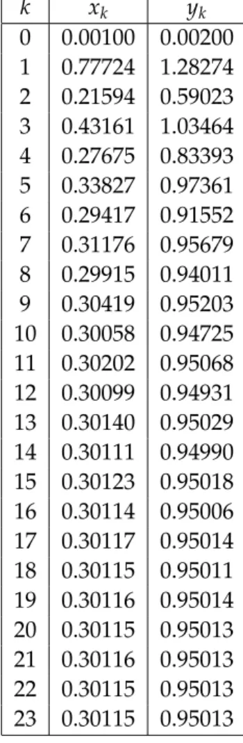
We computed the sequence defined by the iteration (3.26)–(3.27) starting from the initial value (x0,y0) = (0.001, 0.002). The first 23 terms of this sequence are displayed in Table3.2. We can observe that the sequence is convergent, and its limit is(x∗,x∗)≈(0.30115, 0.95013). Therefore Corollary 3.6 yields (3.25) with x∗ ≈ 0.30115 and x∗ ≈ 0.95013. We plotted the numerical solution of equation (3.22) in Figure3.2corresponding to the constant initial functions ϕ(t) = 0.2,ϕ(t) = 0.7 and ϕ(t) = 1.4. The horizontal lines in Figure 3.2 correspond to the lower and upper bounds 0.30115 and 0.95013, respectively. The numerical results demonstrate the
theoretical bounds (3.25).
0 10 20 30 40 50
0.4 0.6 0.8 1 1.2 1.4 1.6
Time t
Solution x(t)
Figure 3.2: Numerical solution of equation (3.22).
4 Proofs
In this section we present the proofs of our main results. First we recall the next lemma from [13], which is needed in our proofs later.
k xk yk 0 0.00100 0.00200 1 0.77724 1.28274 2 0.21594 0.59023 3 0.43161 1.03464 4 0.27675 0.83393 5 0.33827 0.97361 6 0.29417 0.91552 7 0.31176 0.95679 8 0.29915 0.94011 9 0.30419 0.95203 10 0.30058 0.94725 11 0.30202 0.95068 12 0.30099 0.94931 13 0.30140 0.95029 14 0.30111 0.94990 15 0.30123 0.95018 16 0.30114 0.95006 17 0.30117 0.95014 18 0.30115 0.95011 19 0.30116 0.95014 20 0.30115 0.95013 21 0.30116 0.95013 22 0.30115 0.95013 23 0.30115 0.95013
Table 3.2: Fixed point iteration (3.26)–(3.27).
Lemma 4.1. Consider the ordinary differential equation
˙
y(t) =β(t)c− f(y(t)), t ≥T≥0 (4.1) with the initial condition
y(T) =y∗, (4.2)
where c ≥ 0, and β ∈ C(R+,R+) with β(t) > 0 for t > 0, R∞
0 β(s)ds = ∞ and f ∈ C(R,R+) satisfies0 = f(0)< f(x1)< f(x2)for0< x1 < x2. Then for any solution y(T,y∗,c)(t)of the IVP (4.1)–(4.2)we have
(i) c>0and0<y∗< f−1(c)yield that
0<y(T,y∗,c)(t)< f−1(c), y˙(T,y∗,c)(t)>0, t≥ T and
tlim→∞y(T,y∗,c)(t) = f−1(c); (ii) y∗ = f−1(c)yields that y(T,y∗,c)(t) = f−1(c), t ≥T;
(iii) c≥0and y∗ > f−1(c)yield that
y(T,y∗,c)(t)> f−1(c), y˙(T,y∗,c)(t)<0, t ≥T and
tlim→∞y(T,y∗,c)(t) = f−1(c).
Proof of Lemma2.1. Let x(t) = x(ϕ)(t) be any solution of the IVP (2.1)–(2.2). Since x(0) = ϕ(0) > 0, there exists a ξ > 0 such that x(t) > 0 for 0 ≤ t < ξ. If ξ = ∞, then the proof is completed. Otherwise, there exists a t1 ∈ (0,∞) such that x(t) > 0 for 0 ≤ t < t1 and x(t1) = 0. Since α(t)≥ 0 for t ≥ 0 and h(u,v)≥ 0 for any (u,v)∈ R+×R+, we have from (2.1) that
˙
x(t)≥ −β(t)f(x(t)), 0≤t≤ t1. (4.3) But from the comparison theorem of the differential equations (see, e.g., [6]), we have
x(t)≥y(t), 0≤t≤t1,
wherey(t) = y(0,ϕ(0), 0)(t) is the positive solution of (4.1), with c = 0, T = 0 and with the initial condition
y(0) =x(0) = ϕ(0)>0.
Then at t = t1 we get x(t1) ≥ y(t1) > 0, which is a contradiction with our assumption that x(t1) =0. Hence x(t)>0 fort ∈R+.
Proof of Lemma2.2. First, we prove part (i). Consider first equation (2.8) and fix an x ≥ 0.
Sinceg(0,x) =0, limy→∞g(y,x) =∞, andg(·,x)is a strictly monotone increasing continuous function, there exists a unique y > 0 such that g(y,x) = m. Thus there exists a function y=s(x)such thats :R+→(0,∞)satisfies
g(s(x),x) =m, x ≥0. (4.4)
We claim thatssatisfies the following properties:
(i) sis strictly monotone decreasing, (ii) sis continuous onR+,
(iii) limx→∞s(x) =0.
To prove (i), let 0≤x1< x2, then we get
m= g(s(x1),x1)< g(s(x1),x2). But
m= g(s(x2),x2)< g(s(x1),x2),
thus the strict monotonicity of g in its first variable yields s(x2) < s(x1), and hence s(x) is strictly monotone decreasing. To show (ii), letxnbe a strictly monotone increasing sequence of nonnegative numbers such that limn→∞xn=x. Thens(xn)is a monotone decreasing sequence by part (i), so it has a limit, say limn→∞s(xn) = A. Since we have xn < x, thens(xn)> s(x), and so A ≥ s(x). Suppose s(x) < A, we have m = g(s(xn),xn)for all n. Taking the limit as n→∞gives
m= g(A,x)>g(s(x),x) =m.
This contradiction yields that limn→∞s(xn) = s(x). Similarly for any monotone decreasing sequencexnconverging tox, we can show that limn→∞s(xn) =s(x). Hences(x)is continuous on R+. To prove (iii), suppose thats(x)≥ B > 0 for x >0. Then, the monotonicity of g and (2.11) yield
m= g(s(x),x)≥g(B,x)→∞ asx→∞, which is a contradiction, and hence limx→∞s(x) =0.
Now, consider equation (2.7) and fix anx≥0. Theng(x,·)is a strictly monotone increasing continuous function which tends to∞at∞by (2.11). Thus equation (2.7) has a unique solution yif and only ifg(x, 0)≤m. But g(·, 0)is a strictly monotone increasing function which tends to ∞at∞andg(0, 0) =0. Therefore there exists a positive constantxm such that g(x, 0)≤ m for x ∈ (0,xm]. Hence for any x ∈ (0,xm] there exists a unique y ≥ 0 such that (2.7) holds.
This implies that there exists a functiony=r(x)satisfying
g(x,r(x)) =m, x∈(0,xm]. (4.5) We claim thatr satisfies the following properties:
(i) r is strictly monotone decreasing, (ii) r is continuous on(0,xm],
(iii) r(xm) =0,
(iv) limx→0+r(x) =∞.
The proofs of (i) and (ii) are similar to that for the function s, so they are omitted here. Part (iii) is clear from the above definitions ofr. To prove (iv), suppose thatr(x)≤C, whereC>0.
Then, using (2.9) and (4.5),
m= g(x,r(x))≤g(x,C)→0 asx →0, which is a contradiction, since m>0, and hence (iv) is proved.
The above properties of the functions r and s imply that their graphs have at least one intersection, i.e., there exists anxsuch thatr(x) =s(x). See Figure4.1for a possible situation of the graphs. Hence the system (2.7) and (2.8) has at least one positive solution. Let x∗ = inf{u : (u,v)is a positive solution of (2.7) and (2.8)}, and lety∗ = s(x∗). Clearly,(x∗,y∗)is a positive solution of (2.7) and (2.8). The monotonicity of r and s imply that y∗ ≥ v for any solution (u,v) of the system (2.7) and (2.8), so(x∗,y∗) is the dominant solution of (2.7) and (2.8).
Next, we prove part (ii). Consider first inequality (2.13) and we claim that (2.13) is satisfied if and only ify≤s(x). To prove this claim, suppose thaty≤s(x). Then
g(y,x)≤ g(s(x),x) =m.
On the other hand ify>s(x), then
g(y,x)> g(s(x),x) =m.
Thus our claim is proved.
(x*,y*) r(x)
s(x) xm
Figure 4.1: A possible graphs ofs(x)andr(x).
Now, we consider inequality (2.12) and we claim that that (x,y)is a positive solution of (2.12) if and only if [y ≥ r(x) and x ∈ (0,xm]] or [x > xm and y > 0]. To prove the claim, suppose thaty≥r(x)andx∈(0,xm], then
g(x,y)≥g(x,r(x)) =m.
On the other hand ify<r(x), then
g(x,y)<g(x,r(x)) =m.
Supposex>xm andy>0. Then, using the strict monotonicity ofgin both variables, we get g(x,y)> g(xm,y)>g(xm, 0) =g(xm,r(xm)) =m.
Thus our claim is proved.
Clearly, all points of the region A= {(x,y):x > xm and 0< y<s(x)}give us a positive solution of the system (2.12) and (2.13), and the property limx→∞s(x) =0 yields that for any M >0 and ε> 0 there exists(x,y) ∈ Asuch that x > Mand y< ε. Hence, the definition of the dominant solution completes the proof of part (ii).
Proof of Lemma2.3. Let ϕ∈C+be an arbitrary fixed initial function and x(t) =x(ϕ)(t)be any solution of the IVP (2.1)–(2.2). Then, by Lemma 2.1, we have x(t) > 0 for t ≥ 0. We claim that there exist positive constantsd > 0 and d∗ > 0 such that the following inequalities are satisfied,
0min≤t≤δ
x(t)>d, max
0≤t≤δ
x(t)<d∗, α(t)
β(t)h(d,d∗)> f(d) and α(t)
β(t)h(d∗,d)< f(d∗), t ≥δ.
(4.6)
The last two inequalities in (4.6) follow if sup
t≥δ
α(t)
β(t) < f(d∗)
h(d∗,d) (4.7)
and
inft≥δ
α(t)
β(t) > f(d)
h(d,d∗). (4.8)
We define the function
g(x,y) ( f(x)
h(x,y), x>0, y≥0,
0, x=0, y≥0. (4.9)
The assumed monotonicity of hf((x,yx)) in its both variables implies easily thatgis continuous on R+×R+. Then Lemma 2.2 with m = supt≥δ αβ((tt)) and m = inft≥δ
α(t)
β(t) yields that there exist positive numbersdandd∗satisfying the system of inequalities (4.7)–(4.8), max0≤t≤δx(t)<d∗ and min0≤t≤δx(t)>d.
We show thatd <x(t)<d∗ for allt ≥0. Suppose in contrary that there exists t2 ∈ (δ,∞) such thatd< x(t)<d∗fort ∈[0,t2)and either
(i) x(t2) =dor (ii) x(t2) =d∗.
First, consider case (i). Then ˙x(t2)≤ 0. On the other hand, the mixed monotonicity ofh and (4.6) yield that
˙
x(t2) =β(t2) α(t2)
β(t2)h(x(t2−τ),x(t2−σ))− f(x(t2))
≥β(t2) α(t2)
β(t2)h(d,d∗)− f(d)
>0,
which is a contradiction, since ˙x(t2) ≤ 0. Thereforex(t) > d for all t ≥ 0, and hence (2.14) holds.
Next, consider case (ii). Then ˙x(t2)≥ 0. On the other hand, the mixed monotonicity ofh and (4.6) yield that
˙
x(t2) =β(t2) α(t2)
β(t2)h(x(t2−τ),x(t2−σ))− f(x(t2))
≤β(t2) α(t2)
β(t2)h(d∗,d)− f(d∗)
<0,
which is a contradiction, since ˙x(t2) ≥ 0. Therefore x(t) < d∗ for all t ≥ 0, and hence (2.15) holds.
Proof of Theorem2.4. Let x(t) be any fixed solution of the IVP (2.1)–(2.2), and introduce the short notations
x(∞):=lim inf
t→∞ x(t) and x(∞):=lim sup
t→∞
x(t).
Lemma 2.3 implies that 0 < x(∞) ≤ x(∞) < ∞. Moreover, for any T ≥ δ, the constants defined by
aT := inf
t≥Tx(t)≤sup
t≥T
x(t) =: AT (4.10)
and
mT := inf
t≥T
α(t)
β(t) ≤sup
t≥T
α(t)
β(t) =: MT (4.11)
are positive and finite. By (4.10), (4.11) and the mixed monotonicity of h, we get from (2.1) that
˙
x(t)≥β(t)[mTh(aT,AT)− f(x(t))], t≥ T. (4.12) From (4.12) and the comparison theorem of differential equations we see that
x(t)≥y(t) fort ≥T,
wherey(t) =y(T,x(T),mTh(aT,AT))(t)is the solution of equation (4.1) withc=mTh(aT,AT) and with the initial condition
y(T) =x(T). From Lemma4.1, we see that
y(∞):= lim
t→∞y(t) = f−1(mTh(aT,AT)). Thus
f−1(mTh(aT,AT)) =y(∞)≤x(∞), T ≥δ, and from the last inequality, we have
Tlim→∞ f−1(mTh(aT,AT))≤x(∞). Using relations
Tlim→∞aT = x(∞), lim
T→∞AT = x(∞) and lim
T→∞mT = m and the continuity of f−1 andh, we obtain
Tlim→∞f−1(mTh(aT,AT)) = f−1(lim
T→∞mTh(aT,AT)) = f−1(mh(x(∞),x(∞))). Therefore we get
f−1(mh(x(∞),x(∞)))≤ x(∞), and hence
mh(x(∞),x(∞))≤ f(x(∞)). (4.13) In a similar way we can obtain the relation
mh(x(∞),x(∞))≥ f(x(∞)). (4.14) Since x(∞) and x(∞) are positive, (H2) yields h(x(∞),x(∞)) > 0 and h(x(∞),x(∞)) > 0.
Hence (4.13) and (4.14) are equivalent to the system of inequalities f(x(∞))
h(x(∞),x(∞)) ≥ m (4.15)
f(x(∞))
h(x(∞),x(∞)) ≤ m. (4.16)
Define the function g by (4.9). Then g is continuous on R+×R+, and (x(∞),x(∞)) is a solution of the corresponding system of inequalities (2.12)–(2.13). Therefore Lemma 2.2 im- plies (2.17), where(x∗,x∗)is the dominant positive solution of (2.7)–(2.8), or equivalently, the dominant positive solution of the system (2.18)–(2.19).