The 2D time-dependent similarity transformation model as a tool for deformation monitoring

O R I G I N A L S T U D Y

The 2D time-dependent similarity transformation model as a tool for deformation monitoring

Dimitrios Ampatzidis^1•Christian Gruber^2•Vasileios Kampouris³

Received: 23 February 2017 / Accepted: 11 August 2017 / Published online: 24 August 2017 Akade´miai Kiado´ 2017

Abstract Besides the methodology of triangulation and geodetic networks nowadays, the permanent stations of satellite receivers exist, giving extra asset to geodetic daily practice.

Permanent stations perform observations incessantly for the visible satellites. However, the coordinates of these stations are often changing over time due to geophysical and tectonic processes. Consequently, these changes are perceived to modern observations. So, along with the coordinates of geodetic points in a given epoch, their changes over time (e.g. the velocities of their movements) are also considered. Furthermore, any change to the ref- erence system definition or/and to the network’s geometry can significantly impact the estimated coordinates and velocities. This paper investigates the reference datum definition problem (or datum problem, or zero order design problem) in a such network over time, which is later generalized for the study of the deformation control-networks. Emphasis is given to techniques of time-dependent 2D transformation models, with numerical tests on a simulation network.

Keywords VelocitiesDeformationsMonitoringControl networksTime-depended transformation modelsSimulations

& Dimitrios Ampatzidis

Dimitrios.Ampatzidis@bkg.bund.de

1 Federal Agency for Cartography and Geodesy (BKG), Richard-Strauss-Allee 11, 60598 Frankfurt Am Main, Germany

2 German Center for Geosciences (GFZ), Mu¨ncher Str. 20, 82234 Weßling, Germany

3 Laboratory of Geodesy and Geomatics, Aristotle University of Thessaloniki, University Campus, 54124 Thessaloniki, Greece

https://doi.org/10.1007/s40328-017-0205-9

1 Introduction

The 2D similarity transformation has a wide range of applications to classical and engi- neering geodesy. Its main scope is the connection between two different reference systems in terms of translations, scale and orientation. An advantage of the 2D transformation is the absence of the height information and thus there is no assumption for the associated height system (orthometric or/and geometric one) required. This can be useful e.g. when we combine classical with GNSS networks, respectively. In advance, the GNSS-derived heights are less accurate compared to the horizontal coordinates, respectively. On the other hand, the 2D similarity transformation cannot be applied rigorously for relatively large areas (e.g. more than few kilometers). While the spatial (coordinate) transformation is a straightforward procedure, the associated model for 2D velocity transformation is usually omitted. However, in various geodetic monitoring applications the 2D velocity transfor- mation can be needed (e.g. Doukas et al.2004).

The main issue is to connect in an optimal way the coordinates and the estimated velocities through a unified algorithm. For example, this may be required in cases that:

• we have two or more different network realizations at the same area, such an old geodetic monitoring network (realized from classical observations) and a GNSS network which share only a number of common points. Especially for the GNSS network, one should pay great attention, since the observations have completely different nature from the classical one.

• some of the control benchmarks of a network are missing and there is the need of handling and restoring the monitoring information.

• we want to connect two different realizations of the same network: For example, if we aim to quantify the spatial and dynamic inconsistencies from different constraints handling (e.g. Rossikopoulos1986; Dermanis1987; Rossikopoulos1999).

• we test if one or both of the networks carries some systematic errors or blunders.

Thus, we should build a methodology on the optimal combination of the coordinates and velocities of different network realizations. The present study is dedicated to obtain a new methodology dealing with the simultaneous estimation of the spatial and dynamic parame- ters. All the necessary formulas are given and in addition a numerical example is performed.

We must note that till now, there is no published mathematical model for the trans- formation of the 2D (horizontal) velocities. In the majority of the cases, the dynamic part of the network (the velocities) is ignored, and only the classical spatial 2D similarity transformation is applied. This fact can lead to misinterpretations, since the estimated parameters absorb not only the spatial change but in addition, the deformation part which is related to the velocity estimation. The present paper aims to treat this problem, by pro- viding all the mathematical tools and pointing out some crucial theoretical aspects.

The novelty of the proposed approach/strategy lies in the fact that it allows the simultaneous 2D similarity transformation both for coordinates and velocities. Till now, the similarity transformation refers only to the full 3D case (the so-called time-dependent 3D transformation, see e.g. Altamimi et al.2002). In addition, the described approach gives for the first time the necessary mathematical formulas for the 2D similarity transformation of the (plane) velocities. Finally, we should mention that the use of the 3D time-dependent transformation can be problematic in relative small areas, due to the high correlations among the translations, rotations and scale (and their rates). On the other hand, the 2D similarity transformation fits better to limited areas. Thus, the 2D time-dependent trans- formation can stand as an optimal choice for deformation networks in relative small areas.

2 Methodology

The classical 2D similarity transformation has the well known form (e.g. Torge2001):

Xi¼lcoshx_iþlsinhy_iþtx

Yi¼ lsinhx_iþlcoshy_iþty

...

Xn¼lcoshx_nþlsinhy_nþtx

Yn¼ lsinhx_nþlcoshy_nþty

ð1Þ

whereðxi;yiÞ;ðXi;YiÞare the planar coordinates in the initial and the final reference sys- tem, respectively at a pointi,tx;ty are the translations of the initial reference system with respect to the final one,landhare the scale and the rotation parameters, respectively. For simplicity reasons, we can combine the scale and rotation terms as follows (Dermanis and Fotiou1992):

c¼lcosh ð2aÞ

d¼lsinh ð2bÞ

However, the coordinates of both reference systems are inevitably affected from errors.

Thus, the observed planar coordinates are expressed through the following relations (pointwise):

X^b_i ¼XiþeXi ð3aÞ

Y_i^b¼YiþeYi ð3bÞ

x^b_i ¼xiþexi ð3cÞ

y^b_i ¼yiþeyi ð3dÞ

where the termestands for the error of each coordinates component and the superscriptb denotes the observed quantities, respectively. Combining Eqs. (2) and (3), Eq. (1) now yields:

X_i^beXi ¼c x^b_i exi

þd y^b_i eyi

þtx

Y_i^beYi ¼ d x^b_i exi

þc y^b_i eyi

þty

...

X_n^beXn¼c x^b_nexn

þd y^b_neyn

þtx

Y_n^beYn¼ d x^b_nexn

þc y^b_neyn

þty

ð4Þ

The velocities are the derivatives of the coordinates with respect to the time (pointwise):

_ xi¼dxi

dt ð5aÞ

_ y_i¼dyi

dt ð5bÞ

X_i¼dXi

dt ð5cÞ

Y_i¼dYi

dt ð5dÞ

According to the same conceptual manner for the effect of the errors to the coordinates (Eq. 3), we can write the same relations for the velocities:

X_^b_i ¼X_iþeX_i ð6aÞ

Y__i^b¼Y_iþeY_i ð6bÞ

x_^b_i ¼x_iþex_i ð6cÞ

_

y^b_i ¼y__iþey__i ð6dÞ

Following the classical differentiating rules for the Eq.4 and taking into account the Eq. (6), we can express the velocity transformation as follows:

X__i^beX_i ¼c x_ ^b_i exi

þd y_ ⁱ_beyi

þc x_^b_iex_i

þdy_^b_i ey__i þt_x

Y__i^beY_i ¼ d x_ ^b_i exi

þc y_ ⁱ_beyi

d x_^b_i ex_i

þc y_^b_i ey_i

þt_y

...

X__n^beX_n¼c x_ ^b_nexn

þd y_ ^b_neyn

þc x_^b_nex_n

þd y_^b_ney_n

þt_x

Y__n^beY_n¼ d x_ ^b_nexn

þc y_ ^b_neyn

d x_^b_nex_n

þc y_^b_ney_n

þt_y

ð7Þ

The dot signs denote the dynamic parameters (four extra parameters). In order to proceed with the least squares adjustment, it is needed to choose which of the existing method- ologies (observation equations, condition equations or mixed model) will apply. A fruitful description of the different adjustment methodologies is given by Dermanis (1976). In our case, since the observations and the parameters are correlated, we should employ the mixed model, which is generally described as follows:

lðw;uÞ ¼0 ð8Þ

wherelrefers to a function of the observation vectorw¼ X^T X_^T x^T x_^T

h iT

and the vector of the unknowns u¼ c d tx ty c_ d_ t_x t_y

T

. In addition, we

have:X¼ X_i^b Y_i^b ... ... X_n^b Y_n^b 2 66 66 66 66 4

3 77 77 77 77 5

,X_ ¼ X_^b_i Y__i^b ... ... X_^b_n Y__n^b 2 66 66 66 66 4

3 77 77 77 77 5

,x¼ x^b_i y^b_i ... ... x^b_n y^b_n 2 66 66 66 66 4

3 77 77 77 77 5

,x_¼ _ x^b_i

_ y^b_i

... ... _ x^b_n

_ y^b_n 2 66 66 66 66 4

3 77 77 77 77 5

The final linearized combined model

(for the coordinates and the velocities) has the following form:

w¼KduþBe ð9Þ

wherew¼lðw;u^oÞis the loop closure vector (the superscriptostands for the approximate values of the unknowns) du the corrections term, B the Jacobian matrix _ow^ol, e¼

e^T_X e^T_{_}

X e^T_x e^T_{x_}

h iT

the vector of the observations errors, K¼_ou^ol¼ E~^T G^T h iT

, and

E~¼E^T Z^TT

, Z¼

0 0 0 0

0 0 0 0

... ...

... ...

0 0 0 0

0 0 0 0

2 66 66 4

3 77 77

5. In addition, E¼ x^b

i y^b

i 1 0

x^b_i y^b_i 0 1 x^b_n y^b_n 1 0 x^b_n y^b_n 0 1 2

66 66 66 4

3 77 77 77 5

and

G¼ _

x^b_i y_^b_i 0 0 x^b_i y^b_i 1 0 x_^b_i y_^b_i 0 0 x^b_i y^b_i 0 1

_

x^b_n y_^b_n 0 0 x^b_n y^b_n 1 0 x_^b_n y_^b_n 0 0 x^b_n y^b_n 0 1 2

66 66 66 4

3 77 77 77 5

. In our case, for each pointiwe have

the following four equations:

l1i:X^b

i c^ox^b

i d^oy^b

i t_x^o¼w1i ð10aÞ l2i:Y^b

i þd^ox^b

i c^oy^b

i t^o

y ¼w2i ð10bÞ l3i: _X^b

i c^ox_^b

i c_^ox^b

i d_^oy^b

i d^oy_^b

i t_^o

x ¼w3i ð10cÞ l4i : _Y_i^bþd^ox_^b_i þd_^ox^b_i c^oy_^b_i c_^oy^b_i t_^o_y ¼w4i ð10dÞ Our final model comprises eight transformation parameters: The classical spatially related parameters of the similarity transformation, in addition to their associated trans- formation rates. Note, the velocities are mutually dependent to the eight transformation parameters, though the coordinates are blind to the rate parameters. For the approximate values of the parameters one can initially set all of them as zero, except for thec, which can be one. Of course, after a number of iterations the optimal parameters are estimated (setting each time the previous estimated values as the approximate one).

2.1 The mathematical model for the least squares adjustment

Applying the least squares principle (e.g. Koch1987), the estimated unknown parameters, adjusted observations and adjusted residuals (four for the coordinates and four for the velocities) are derived as follows (e.g. Dermanis and Fotiou1992for the mixed model):

d^u¼ K^TM¹K1

K^TM¹w ð11Þ

the associated covariance matrix is:

Cu^¼r^²K^TM¹K1

ð12Þ The estimated errors,

e^¼CeB^TM¹ðwþKd^uÞ ð13Þ

and r^²¼^{e^}_4n8^{TC1e e^}the a posteriori variance (n the number of the points). Finally, M¼

BC¹_e B^T with Ce¼ CeX

CeX_

Cex

Cex_

2 66 4

3 77

5 the 4n94n covariance matrix of the observation errors (coordinates and velocities). We assume implicitly, that the coordinates and velocities are not correlated. This is a realistic assumption, since the velocities are estimated mainly, by individual time series of the coordinates.

If we want to express the covariance error matrix to a more correct form, we have:

Ce¼ r²₁Q_eX

r²₂Q_{e_}

X

r²₃Q_ex r²₄Q_{ex_} 2

66 4

3 77

5 ð14Þ

wherer²₁;r²₂;r²₃;r²₄are the (unknown) variances of each group of the observations. They can be estimated using the so-called Variance Component Analysis (VCA- see e.g. Ba¨hr et al.2007).

2.2 The case of different realization epochs

It is possible that the two reference systems are not realized in the same epoch. For example, this can occur when the initial network was measured many years before the final one. In this case one should take into account the coordinate change throughout the time. In this case, all the coordinate related quantities, presented in the matricesEandG(Eq.9), respectively should be changed, according to the following expressions:

xi¼x^t_i⁰þx_iðTot0Þ ð15aÞ yi¼y^t_i⁰þy__iðTot0Þ ð15bÞ wherex^t_i⁰;y^t_i⁰the 2D coordinates of the initial frame at the epochtoof its realization andTo

the reference epoch of the final reference frame. By this manipulation, we express the coordinates of the initial system to the realization epoch of the final one. If we ignore this critical modification, the estimated parameters would absorb a kind of pseudo information, which in fact is a bias due to the different realization epochs. This bias can be significant, if the time difference between them is relatively large (e.g. decades) or/and the velocities are also large.

2.3 Some remarks regarding the practical application of the 2D time dependent similarity transformation

(1) The above equations are used for the simultaneous estimation of the parameters connecting the coordinates and the velocities of two different reference systems. We underline again that the 2D similarity transformation is well defined only for limited areas. If one wants to apply the 3D similarity transformations both for coordinates and velocities, Altamimi et al. (2002) give all the necessary mathematical formulas for it. The present study should be considered as the special case of the 3D time- dependent transformation given by Altamimi et al. (2002).

(2) The same concept can be easily implemented to the vertical networks. In this case, we have only two estimated parameters: the offset and its rate.

(3) The time dependent 2D similarity transformation could be expanded for the affine or polynomial transformations, respectively. However, the model will include relative many unknown parameters.

(4) We should be aware of the realization epochs. As we discussed previously, this can distort our results. If the reference epoch is not explicitly defined, we should re- compute the associated networks per epoch. Then, it is needed to define a reference epoch (e.g. in the mean epoch of the observation). Finally, the velocity estimation using e.g. time series analysis should be estimated.

3 Numerical example

Our new approach for the optimal estimation of the spatial and dynamic parameters of the 2D similarity transformation is tested through a simulation paradigm.

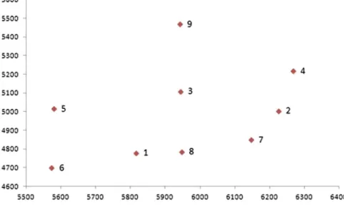
1. Initially, we create a random network of 9 points (Fig.1). We set an initial network of well distributed stations, covering an area of approximately 1 km². From this network, we extract 40 horizontal distances and 26 angles as they derived using the Pythagorean theorem and the the differences of the computed azimuths, respectively. In the case of the horizontal distances, we add zero mean noise with 1.0 mm/yr standard deviation, while for the angles we assume 0.2 mgons standard deviation (again zero mean). For both cases, we used the Matlab random noise generator. The noise level reflects adequately the observational uncertainty of the modern and precise terrestrial measurements used for the deformation monitoring.

2. For these 9 points, we also consider 2D velocities. We artificially generate 18 velocities (x and y components of the 9 points) with the following statistical characteristics: mean average 10 mm/yr and standard deviation 3.0 mm/yr.

Fig. 1 The simulated network

3. The simulated network (initial network) is solved imposing partial inner constraints to the points 1, 3 and 9. The mean standard deviations (mean average of the squared diagonal elements of the covariance matrix of the estimated unknowns, Eq.12, ibid.) are 0.96 mm and 0.13 mm/yr for the coordinates and velocities, respectively.

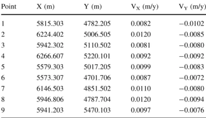
4. In order to compute the final network, we apply the eight similarity transformation parameters (spatial and dynamic). These parameters are designed in a way that realize a reference system which is relatively ‘‘close’’ to the initial one, in terms of translations, scale and orientation (and for their associated rates). Then, we add random noise to the coordinates and velocities for the final reference system. The statistical characteristics of the added noise are zero mean (for both coordinates and velocities) and standard deviations of 1.5 mm and 1.0 mm/yr, respectively. Further- more, for 2 x-components and 2 y-components of the initial network, we add a bias of 5 mm to their noised values. This bias is induced in order to take account of some systematic effects. We assumed both noise and bias for the final network, in order to have a realistic simulation scenario. Tables1 and 2 refer to the coordinates and velocities of the initial and final reference system, respectively. Figure2depicts the velocities with respect to the two systems.

We also apply statistical tests to our results (Koch1987). We implement the two-sides F-test (testing the variances) and the Student test (ttest) for outlier detection for the initial and the final network, respectively.

Table 1 The coordinates and the velocities of the initial refer- ence system

The coordinates are in meters and the velocities are in meters/yr

Point X (m) Y (m) Vx(m/y) Vy(m/y)

1 5815.301 4782.201 0.0086 -0.0102

2 6224.399 5006.500 0.0105 -0.0103

3 5942.299 5110.501 0.0092 -0.0104

4 6266.600 5220.100 0.0097 -0.0100

5 5579.299 5017.201 0.0110 -0.0090

6 5573.299 4701.701 0.0089 -0.0082

7 6146.501 4851.500 0.0113 -0.0094

8 5946.800 4787.699 0.0107 -0.0103

9 5941.200 5470.099 0.0099 -0.0093

Table 2 The coordinates and the velocities of the final refer- ence system

Point X (m) Y (m) VX(m/y) VY(m/y)

1 5815.303 4782.205 0.0082 -0.0102

2 6224.402 5006.505 0.0120 -0.0085

3 5942.302 5110.502 0.0081 -0.0080

4 6266.607 5220.101 0.0092 -0.0092

5 5579.303 5017.205 0.0099 -0.0083

6 5573.307 4701.706 0.0087 -0.0072

7 6146.503 4851.502 0.0110 -0.0080

8 5946.806 4787.704 0.0120 -0.0094

9 5941.203 5470.103 0.0097 -0.0076

Regarding the covariance matrix of the observation errors, we use the covariance matrix of estimated coordinates, and a unity matrix for the velocities. For the velocities, the unity matrix was multiplied by a factor of 1910^-6, assuming implicitly that the velocities were estimated with a formal error of 1 mm/yr. We should note here that since the network is solved using inner constraints, the associated covariance matrix of the coordinates is singular (e.g. Koch1987). We overcame this problem, by slightly modifying the covari- ance matrix by adding a diagonal matrix, as follows (Bjerhammar 1973; Sillard and Boucher2001; Rossikopoulos2001):

Cx^¼Cx^þdI ð16Þ

whereCx^is the covariance matrix of the estimated coordinates and 0\d1. In our case, we haved=0.00001.

The results of the implementation of the combined 2D similarity transformation are presented in the following tables. Table3 shows the estimated parameters and their associated formal errors, while Table4refers to the residual statistics for the coordinates and velocities.

Fig. 2 The simulated velocities of the two systems

Table 3 The estimated parame- ters and their associated formal errors

Parameter Values

c 0.99999720486±2e-07

d -1.7277e-07±5e-07

tx 0.0219±0.015 m

ty 0.0164±0.012 m

_

c 2.2681 e-06±3.2e-07

d_ -3.419e-08±1.2e-08

t_x 0.0067±0.0028 m/yr

t_y -0.0103±0.009 m/yr

The standard deviation of the residuals (0.0017 m and 0.0010 m/yr, respectively) is at the level of our initial formal error assumptions (the assumptions regarding the added random noise to the observations). Furthermore, the mean residual average is practical zero.

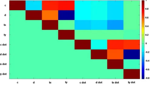
Finally, Fig.3shows the correlations between the estimated parameters. Correlations are estimated directly from the covariance matrix of the estimated unknown parameters.

Observing Fig.3, we imply that there are strong correlations ([0.8) between some parameters. The largest correlations are found between:

• the parametercand the translationstx;ty

• thec_and the dynamic translationst_x;t_y

• thed_and the dynamic translationt_y

These correlations might be caused due to the relatively small network area and in top of that, the origin of the reference system is almost 6 km away from the network. It is worth to mention that there is no significant cross-correlation between the spatial (referring to the coordinates) and the dynamical (referring to the velocities) parameters. We should always take into consideration the correlation between the estimated parameters. Large correlation could reveal some problems which probably distort the transformation.

Table 4 The residuals of the coordinates and the velocities, after the application of the 2D time dependent similarity transformation

Quantity Coordinates Velocities

Min -0.0027 -0.0021

Max 0.0027 0.0027

Std 0.0017 0.0010

Mean 0.0001 0.0000

The coordinates are in meters and the velocities are in meters/yr

Fig. 3 The correlations between the estimated parameters

However, we must keep in mind that the 2D similarity transformation is applied to limited areas, a fact that increases the correlations.

4 Conclusions and further investigations

At the present study, we discussed a new approach on the optimal 2D similarity trans- formation, using coordinates and velocities. We provide all the necessary formulas and we test them through a simulation network. The new methodology could be useful in various geodetic and surveying applications, like:

1. Connecting two different dynamic networks established for geodetic monitoring (e.g.

fault or dam monitoring or even for an industrial application). This could be useful, because for the aforementioned cases, the velocities play a crucial role for the safety of the people and the constructions.

2. Assimilating the information from a tectonic plate model, with results derived from geodetic measurements. This could lead to the improvement of local deformation models through the use of global solutions. In addition, it can be considered as a tool on the assessment of the tectonic plate models by the use of local precise geodetic networks.

3. In cases where the height information is rather problematic and it is possible to distort the results. Our methodology does not imply any height handling and thus it can be applied independently. Furthermore, the precise height estimation needs for the most of the cases geometric levelling measurements which increase the time and the cost of our work.

4. For the comparison of the results between the 3D and 2D time dependent transformation models regarding the horizontal velocities. E.g. how the height related information affects on the horizontal plane deformation estimation. This can be done by applying independently the 3D and 2D time-dependent transformation, respec- tively. Then one can compare the horizontal coordinate residuals after the implemen- tation of the two different transformations mentioned before.

5. In cases where it is necessary to investigate if there is consistency between different types of observations from which the horizontal deformations are determined. E.g. if GNSS scale (and its rate) is consistent to the total station derived one, respectively.

This can be important, since the older classical networks define their scale using terrestrial distance measurements.

The new methodology was tested through a simulation network. The simulated network was designed as a precise network for deformation monitoring. We followed rigorous statistical tests in order to reject possible blunders. Applying the 2D similarity time- dependent transformation, we conclude that it provides the necessary information for the reliable spatial and dynamic connection between two reference systems. The standard deviation of the coordinate residuals and velocities lay at 1.7 mm and 1.0 mm/yr, respectively.

Of course, the new methodology should be implemented with real observations and reference systems in order to clarify and further investigate the results, especially the correlations of the estimated parameters. We should again note that the 2D similarity transformation offers reliable results only in limited areas. The results of the proposed

approach should be definitely compared with those of the other strategies that are already applied for the deformation studies.

Acknowledgements Professor I.D Doukas is kindly acknowledged for his suggestions and comments. Dr.

Dipl. Ing. Grigorios Tsinidis (Department of Geotechnical Works/Aristotle University of Thessaloniki) gave some hints on the handling of Matlab scripts for random noise implementation and some ideas for the deformation modeling. The comments and the suggestions of the three anonymous reviewers led to the significant improvement of the initial manuscript.

References

Altamimi Z et al (2002) ITRF2000: A new release of the international terrestrial reference frame for earth science applications. J Geophys Res. doi:10.1029/2001JB000561

Ba¨hr H, Altamimi Z, Heck B (2007) Variance component estimation for combination of terrestrial reference frames, Universita¨t Karlsruhe Schriftenreihe des Studiengangs Geoda¨sie und Geoinformatik, ISBN:

978-3-86644-206-1

Bjerhammar A (1973) Theory of errors and generalized matrix inverses. Elsevier, Amsterdam

Dermanis A (1976) Probablistic and deterministic aspects of linear estimation in geodesy. Ph.D. Thessis, Report 244, Ohio State University

Dermanis A (1987) Adjustment of observations and estimation theory, vol 2. Ziti Publications, Thessaloniki, p 311(in Greek)

Dermanis A, Fotiou A (1992) Adjustment methods and applications. Ziti Publications, Thessaloniki, p 348 (in Greek)

Doukas I, Fotiou A, Ifadis IM, Katsambalos K, Lakakis K, Petridou- Chrysohoidou N, Pikridas C, Ros- sikopoulos D, Savvaidis P, Tokmakidis K, Tziavos IN (2004) Displacement field estimation from GPS measurements in the Volvi area. In: Proceedings of FIG 27th working week ‘‘The Olympic Spirit in Surveying’’, Athens, Greece, 22–27 May (CD-ROM)

Koch K-R (1987) Parameter estimation and hypothesis testing in linear models. Springer, Berlin, p 378 Rossikopoulos D (1986) Integrated control networks. Ph.D. Dissertation. Aristotle University of

Thessaloniki

Rossikopoulos D (1999) Surveying networks and computations, vol 2. Ziti Publications, Thessaloniki, p 420 (in Greek)

Rossikopoulos D (2001) Modeling alternatives in deformation measurements. In: Carosio A, Kutterer H (eds) First International Symposium on Robust Statistics and Fuzzy Techniques. ETH, Zurich Sillard P, Boucher C (2001) A review of algebraic constraints in terrestrial reference frame datum definition.

J Geodesy. doi:10.1007/s001900100166 Torge W (2001) Geodesy, 3rd edn. de Gruyter, Berlin