Similarity transformation approach for a heated ferrofluid flow in the presence of magnetic field
Dedicated to Professor László Hatvani on the occasion of his 75th birthday
Gabriella Bognár
Band Krisztián Hriczó
University of Miskolc, Miskolc-Egyetemváros, Miskolc, H–3515, Hungary Received 13 January 2018, appeared 26 June 2018
Communicated by Tibor Krisztin
Abstract. The aim of this paper is to investigate theoretically the magneto- thermomechanical interaction between a heated viscous incompressible ferrofluid and a cold wall in the presence of a spatially varying field. Similarity transformation is used to convert the governing non-linear boundary-layer equations into coupled non- linear ordinary differential equations. These equations are numerically solved using a discretization scheme using higher derivative method (HDM). The effects of governing parameters corresponding to various physical conditions are analyzed. Numerical re- sults are obtained for distributions of velocity and temperature, the dimensionless wall skin friction and heat-transfer coefficients. The results indicate that two solution exists in some cases. A comparison with previous studies available in the literature has been done and we found an excellent agreement with it.
Keywords: similarity transformation, ferrofluids, boundary layer, Blasius equation.
2010 Mathematics Subject Classification: 76D05, 34A34, 35G45.
1 Introduction
There is a necessity to develop novel types of fluids for technological, biomedical and aero- space areas. Magnetic nanofluids are important functional fluids. Magnetic fluids, also called ferrofluids, are stable colloidal suspensions of non-magnetic carrier liquid, typically water, ethylene glycol, glycerol or oil, containing very fine magnetized particles, for example mag- netite, with diameters of order 5–15 nm [22].
One of the most important features of ferrofluids is the ability to change their physical properties by means of magnetic fields. In recent years, this capability makes ferrofluids very useful in the fields of engineering and fundamental research. Such suspensions behave like a normal fluid and act as a ferromagnetic material.
Ferrofluid has the merits of nanoparticles in improving the thermal properties of the fluid.
The addition of nanoparticles to the carrier fluid improves the transport properties of the fluid
BCorresponding author. Email: v.bognar.gabriella@uni-miskolc.hu
for example the thermal conductivity and leads to heat transfer enhancement. The velocity and temperature distribution can be altered by applying an external magnetic field. This thermo-magnetic coupling makes ferrofluids useful in various practical applications in indus- trial engineering and technological applications. Such type of applications includes electrical instruments, heat exchanger, vehicle cooling, cooling of electronic devices and vehicle thermal management. Among the engineering applications of ferrofluids are those taking the advan- tage of the application of an external force into the fluid, mainly filtering, percolation, sealing, separation, ink-jet printing and heat transfer [3,8]. Magnetic fluids have also been used in the lubrication of bearings as they have some advantages over conventional lubrication. Several authors have theoretically investigated the characteristics of various bearing configurations using ferrofluid lubricants [24,26].
When magnetizable materials are subjected to an external magnetizing fieldH, the mag- netic dipoles or line currents in the material will align and create a magnetizationM.
In the magnetohydrodynamic theory, the Lorentz force can be non-zero even with the application of a uniform magnetic field. the problem of MHD flow over infinite surfaces has become more important due to the possibility of applications in areas like nuclear fusion, chemical engineering, medicine, and high-speed, noiseless printing. Problem of MHD flow in the vicinity of infinite plate has been studied intensively by a number of investigators (see, e.g., [1,6,7,10,11,13,14,25] and the references therein). The hydrodynamic flow of MHD fluids was studied when the applied transverse magnetic field is assumed to be uniform.
In recent years various theoretical models have been put forward to study the contin- uum description of ferrofluid flow. Most of the analytical studies concerning the motion of ferrofluids are based on the formulation given by either Neuringer and Rosensweig [20] or Shliomis [23]. Neuringer and Rosensweig developed a model, where the effect of magnetic body force was considered under the assumption that the magnetization vectorMis parallel to the magnetic field vectorH.
Andersson and Valnes [5] extended the so-called Crane’s problem by studying the influ- ence of the magnetic field, due to a magnetic dipole, on a shear driven motion, on a flow over a stretching sheet of a viscous non-conducting ferrofluid. The fluid flow was formulated as a system five partial differential equations and the influence of the magneto-thermomechanical coupling was explored numerically. It was shown that the effect of the magnetic field was to decelerate the fluid motion as compared to the hydrodynamic case. In [2] it was concluded that the presence of heat source (or sink) controls the effect of the magneto-thermomechanical interaction, which decelerates the flow along the stretching sheet thereby influence on the heat transfer rate. Zeeshan et al. [28] investigated the effects of magnetic dipole and thermal radiation on the flow of ferromagnetic fluid on a stretching sheet.
Neuringer [21] has examined numerically the dynamic response of ferrofluids to the appli- cation of non-uniform magnetic fields with studying the effect of magnetic field on two cases, the two-dimensional stagnation point flow of a heated ferrofluid against a cold wall and the two-dimensional parallel flow of a heated ferrofluid along a wall with linearly decreasing surface temperature.
The aim of this paper is understanding the static behavior of ferrofluids in magnetic fields.
Similarity transformation is applied on the governing equations to transform partial differen- tial equations to nonlinear ordinary differential equations. A numerical solution is obtained.
Wall shear stress, heat transfer, velocity and temperature boundary layer profiles are obtained and compared with the results obtained in [21]. The behavior of the velocity and thermal distribution is investigated. It will be shown that in some cases two different solutions exist.
y
x a
a
u=uw, T=Tw u=u∞, T=Tc
H=Ha+H-a Ha
H-a
Figure 2.1: Parallel flow along a cold flat sheet in the presence of magnetic field due two line currents.
The effects of the parameters involved in the boundary value problem will be graphically illustrated.
2 Mathematical formulation
Consider a steady two-dimensional flow of an incompressible, viscous and electrically non- conducting ferromagnetic fluid over a flat sheet in the horizontal direction shown in Figure2.1.
The field is due to two line currents perpendicular to and directed out of the flow plane and equidistantafrom the leading edge. The wall temperature is a decreasing temperature and is given by Tw=Tc[1−Axm+1], where Aandmare real constants.
Introducing the magnetic scalar potential φ whose negative gradient equals the applied magnetic field, i.e.H=− ∇φ, the scalar potential can be given by
φ(x,y) =− I0 2π
tan−1 y+a
x +tan−1y−a x
,
where I0 denotes the dipole moment per unit length and a is the distance of the line current from the leading edge. Then, the corresponding field components are given by
Hx =−∂φ
∂x = − I0 2π
"
y+a
x2+ (y+a)2 + y−a x2+ (y−a)2
# , Hy =−∂φ
∂y = − I0 2π
"
x
x2+ (y+a)2 + x x2+ (y−a)2
# . Moreover, the second derivatives are
∂2φ
∂x2 =−∂
2φ
∂y2 =− I0 2π
2x(y+a) h
x2+ (y+a)2i2
+ 2x(y−a) h
x2+ (y−a)2i2
and
∂2φ
∂x ∂y =− I0 2π
(y+a)2−x2 h
x2+ (y+a)2i2
+ (y−a)2−x2 h
x2+ (y−a)2i2
.
In ferrohydrodynamic interactions, the existence of spatially varying fields is required [20].
The following assumptions will be made:
(i) the direction of magnetization of a fluid element is always in the direction of the local magnetic field,
(ii) the fluid is electrically non-conducting and (iii) the displacement current is negligible.
Then the dynamic response of ferrofluids to the application of non-uniform magnetic fields follows from the fact that the force per unit volume on a piece of magnetized material of magnetizationM(i.e. dipole moment per unit volume) in the field of magnetic intensityHis given by the formµ0M∇H, where
H= s
∂φ
∂x 2
+ ∂φ
∂y 2
,
µ0 denotes the free space permeability and M represents the magnitude ofM. Applying the scalar potentialφ, ∇His calculated as follows
∇H=[∇H]x,[∇H]y=
∂φ
∂x
∂2φ
∂x2 +∂φ∂y∂x∂2φ∂y r
∂φ
∂x
2
+∂φ∂y2 ,
∂φ
∂x
∂2φ
∂x∂y+ ∂φ∂y∂∂y2φ2 r
∂φ
∂x
2
+∂φ∂y2
.
Since(∂φ/∂x)y=0=0 and ∂2φ/∂y2
y=0=0 at the wall, then[∇H]y vanishes.
In the boundary layer for regions close to the wall when distances from the leading edge large compared to the distances of the line sources from the plate, i.e.x a, then one gets
[∇H]x =−I0 π
1 x2.
The boundary layer equations for a two-dimensional and incompressible flow are based on expressing the conservation of mass, continuity, momentum and energy. The analysis is based on the following four assumptions [21]:
(i) the applied field is of sufficient strength to saturate the ferrofluid everywhere inside the boundary layer,
(ii) within the temperature extremes experienced by the fluid, the variation of magnetization with temperature can be approximated by a linear equation of state, the dependence of M on the temperature T is described by M = K(Tc−T), where K is the pyromagnetic coefficient and Tc denotes the Curie temperature as proposed in [4,21],
(iii) the induced field resulting from the induced magnetization compared to the applied field is neglected; hence, the uncoupling of the ferrohydrodynamic equations from the electromagnetic equations and
(iv) in the temperature range to be considered, the thermal heat capacity c(1.6–2.2 J/g K), the thermal conductivityk(1–1.6 W/m K), and the coefficient of viscosityν(5–5000·10−6 m2/s) are independent of temperature.
Then, the governing equations are described as follows
∂u
∂x +∂v
∂y =0, (2.1)
u∂u
∂x +v∂u
∂y =−Ioµ0K
πρ (Tc−T)1
x2 +ν∂2u
∂y2, (2.2)
c
u∂T
∂x +v∂T
∂y
=k∂2T
∂y2, (2.3)
where the x and y axes are taken parallel and perpendicular to the plate, u and v are the parallel and normal velocity components to the plate, respectively,νis the kinematic viscosity andρ denotes the density of the ambient a fluid, which will be assumed constant. Equations (2.1)–(2.3) are considered under the boundary conditions at the surface (y=0)
u(x, 0) =0, v(x, 0) =0, T(x, 0) =Tw, (2.4) with Tw= Tc−Axm+1 and
u(x,y)→u∞, T(x,y)→ T∞ (2.5) as y leaves the boundary layer (y → ∞) with T∞ = Tc, and u∞ is the exterior streaming speed which is assumed throughout the paper to be u∞ = U∞xm (U∞ = const.). Parameter mis relating to the power law exponent. The parameterm= 0 refers to a linear temperature profile and constant exterior streaming speed. In case of m = 1, the temperature profile is quadratic and the streaming speed is linear. The value of m = −1 corresponds to no temperature variation on the surface.
Introducing the stream functionψ, defined byu =∂yψandv=−∂xψ, problem (2.1)–(2.3) can be formulated as
∂yψ ∂yxψ−∂xψ ∂yyψ=ν ∂yyyψ− I0µ0K
πρ (Tc−T), (2.6)
c
∂yψ ∂xT−∂xψ ∂yT
=k ∂yyT. (2.7)
Boundary conditions (2.4) and (2.5) are transformed to
∂yψ(x, 0) =0, ∂xψ(x, 0) =0, T(x, 0) =Tc−Axm+1, (2.8)
∂yψ(x,y)→U∞xm, T(x,y) =Tc asy→∞. (2.9) Now, we have two single unknown functions and two partial differential equations. The structure of (2.6)–(2.9) allows us to look for similarity solutions of a class of solutionsψandT in the form (see [9])
ψ(x,y) =C1xbf(η), T=Tc+Axm+1Θ(η), η=C2xdy, (2.10) wherebanddsatisfy the scaling relation
b+d =m
and for positive coefficientsC1andC2the relation C1 C2 = ν
must be fulfilled. The real numbersb,dare such thatb−d=1 andC1C2=U∞, i.e.
b= m+1
2 , d= m−1
2 , C1=√
νU∞, C21 = rU∞
ν .
By taking into account (2.10), equations (2.6) and (2.7) and conditions (2.8) and (2.9) lead to the following system of coupled ordinary differential equations
f000−m f02+ m+1
2 f f0−βΘ=0, (2.11)
Θ00+ (m+1) Pr 1
2 f Θ0−Θ f0
=0 (2.12)
subjected to the boundary conditions
f(0) =0, f0(0) =0, Θ(0) =1, (2.13) f0(η) =1, Θ(η) =0 as η→∞, (2.14) where Pr=cν/kis the Prandtl number and β= I0µ0KA/(πρU2∞).
The components of the non-dimensional velocityv= (u,v, 0)can be expressed by u=U∞ xm f0(η),
v=−√
νU∞ x(m−1)/2
m+1
2 f(η) + m−1
2 f0(η) η
. The shear stress and the heat transfer at the wall are derived
τy=0=νρ ∂u
∂y
y=0
=ρU∞√
νU∞ x3m2−1f00(0),
−k ∂T
∂y
y=0
=−kA rU∞
ν x3m2+1Θ0(0),
where f00(0)denotes the skin friction coefficient andΘ0(0)stands for the heat transfer coeffi- cient.
According to our knowledge, the coupled boundary-layer equations for the case when m= 0 were first examined by Neuringer [21]. Ifm=0 andβ=0, equation (2.11) is equivalent to the famous Blasius equation
f000+1
2 f f0 =0, (2.15)
which appears when studying a laminar boundary-layer problem for Newtonian fluids [12, 14].
In the mathematical study of a model describing the dynamics of heat transfer in an incom- pressible magnetic fluid under the action of an applied magnetic field, the fluid is assumed nonelectrically conducting and the obtained solutions are valid only for distances greater thana.
3 Results and discussion
There are several methods for the numerical solution of boundary value problems of similar type of coupled strongly nonlinear differential equations as (2.11)–(2.12). In [12], the authors applied the successive linearization method to solve the boundary value problem, where the unknown functions are obtained by iteratively solving the linearized version of the governing equation. Using a selection of initial guesses and auxiliary linear operators is quite essential to find the homotopic solutions for flow analysis [18]. Tzirtzilakis et al. [27] obtained numerical results by a numerical technique based on the common finite difference method. Zeeshan et al. [28] and Abraham et al. [2] solved the highly non-linear differential equation subjected to boundary conditions by shooting method when the higher-order ordinary differential equa- tions are converted into the set of first-order simultaneous equations, which can be integrated as an initial value problem using the well known Runge–Kutta Fehlberg fourth-order scheme.
The initial guesses for the unknown functions were adjusted iteratively by Newton–Raphson’s method.
In this paper, the coupled ordinary differential equations (2.11)–(2.12) are solved numeri- cally with boundary conditions using higher derivative method (HDM) with A-stability prop- erty. The algorithm of HDM is implemented in Maple by Chen et al. [16]. After the implemen- tation, the algorithm is shared as an open access Maple code. Their implementation is able to determine efficient solution to boundary value problems, which are described by ordinary differential equations.
Although, there are numerous numeric solving program, this code plays a very impor- tant role in the numerical analysis of boundary value problems because it can be possible to realize increasing accuracy while ensuring stability by using higher derivatives [17]. In the manuscript [16], a detailed description and several examples are given that prove its widespread applicability. It is necessary to note that this source code works from Maple 8 up to the latest version.
The discretization of boundary value problems based on HDM scheme. The concept of HDM scheme originates from the stability function of A-stable implicit Runge–Kutta meth- ods, for example, Gauss–Legendre methods and Lobatto IIIA methods. It operates nth order derivative to receive 2n order of accuracy at each node point. The implemented method contains two routines that can be called by the user: (1) Procedure HDM (2) Procedure HD- Madapt. The HDM procedure returns the solutions based on a given mesh and order, while HDMadapt procedure returns the solutions with automatically adjusted mesh and order [16].
It is experienced that most of the test runs quickly, in a few seconds, i.e., the calculation time is short.
A discretization scheme using higher derivative method (HDM) suggested by Chen et al.
[16] is applied for the solution of the boundary value problem (2.11)–(2.14). The setting of digits in our case is digits = 15. The boundary value problem is considered as a system of first order ordinary differential equations:
diff(y1(x),x) =y2(x), diff(y2(x),x) =y3(x),
diff(y3(x),x) =m∗y2(x)∗y2(x)−(m+1)/2∗y1(x)∗y3(x) +β∗y4(x), diff(y4(x),x) =y5(x),
diff(y5(x),x) =−Pr∗((m+1)/2∗y1(x)∗y5(x)−(m+1)∗y4(x)∗y2(x)), wherey1(x) = f(η)andy4(x) =Θ(η).
The left and right boundary conditions are defined bybc1 andbc2, respectively bc1 := evalf([y1(x),y2(x),y3(x)−B,y4(x)−1,y5(x)−C]), bc2 := evalf([y2(x)−1,y4(x)]),
where BandC are unknown parameters. It is necessary to give the range (bc1 tobc2) of the boundary value problem (Range := [0.,ηmax]). We have three parameters, m, β and Pr (e.g., pars := [m = 0.0,b = 0.0, Pr= 10.0]), and two unknown B andC (unknownpars := [B,C]).
The next step is to define the initial derivative in nder and the number of the nodes in nele (nder :=3; nele :=5;). Next settings of the absolute and relative tolerance for the local error are (atol :=1e−6; rtol :=atol /100;). The HDM adapt procedure is applied to determine the approximate numeric solution. The simulation gives the value of unknown parametersBand C, and then we get the figure of all solution functions (fromy1 toy5).
During our investigations, the velocity and temperature changes in the boundary layer are examined and the effects of the parameters on the solution are illustrated in the figures.
Studies conducted by Neuringer [21] on the ferrofluid flow indicated that the decrease of the f00(0) and Θ0(0)with increasing β is slightly non-linear. Our numerical solutions for the same parameters β, Pr = 10 and m = 0 as obtained in [21] are presented in Table 3.1 applying the same length for ηmax = 6. The Prandtl number Pr = 10 is fixed as a typical value of kerosine based ferrofluid. The comparison of the values of the dimensionless wall skin friction and heat-transfer coefficients, f00(0) and Θ0(0), shows good agreement. The effect of parameterβon the nondimensional velocity and thermal distribution is exhibited on Figs.3.1–3.2.
f00(0) Θ0(0)
β [21] present [21] present
0.00 0.3020 0.332566 −1.1756 −1.176316 0.05 0.3058 0.305901 −1.1557 −1.155898 0.10 0.2782 0.278368 −1.1338 −1.134037 0.15 0.2497 0.249826 −1.1102 −1.110458 0.20 0.2199 0.220084 −1.0845 −1.084788 0.25 0.1887 0.188882 −1.0561 −1.056504 0.30 0.1556 0.155840 −1.0244 −1.024832 0.35 0.1201 0.120373 −0.9881 −0.988552 0.40 0.0811 0.081472 −0.9449 −0.945512
Table 3.1: f00(0)andΘ0(0).
Unlike initial value problems, where a unique solution can be guaranteed with initial con- ditions of differential variables, boundary value problems sometimes have the situation that either no solution or multiple solutions exist even for the simple set of differential equations (see [15] and [19]). Applying the HDM method on different length of intervalsηmaxintroduces the existence of two solutions: an upper and a lower solution for f0 and also two correspond- ing solutions for the nondimensional temperature profile. Table 3.2 lists the values of the dimensionless wall skin friction and heat-transfer coefficients, f00(0) and Θ0(0) respectively, depending on the parameterβ. It is also indicated that the corresponding length of interval is different for different values ofβ.
type I. type II.
β f00(0) Θ0(0) ηmax f00(0) Θ0(0) ηmax 0.05 0.305507 −1.155421 6.5 −0.148283 2.981088 6.6 0.10 0.277750 −1.133269 8.0 −0.162851 1.301214 8.1 0.15 0.249132 −1.109570 8.1 −0.178707 0.770688 8.3 0.20 0.219295 −1.083745 8.3 −0.190675 0.467910 8.4 0.25 0.187974 −1.055260 8.0 −0.199114 0.257365 8.2 0.30 0.154770 −1.023305 8.0 −0.203945 0.091868 8.2 0.35 0.120373 −0.988552 6.0 −0.207633 −0.033516 6.5 0.40 0.081472 −0.945512 6.0 −0.203722 −0.165718 6.5 0.45 0.035499 −0.888527 6.5 −0.191647 −0.301338 6.9 0.50 −0.021471 −0.807126 6.5 −0.1681002 −0.445667 6.8
Table 3.2: Two types of solutions obtained by HDM Maple.
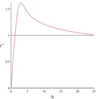
The ferromagnetic parameter β highlights the effect of the external magnetic field. The dimensionless velocity decreases with an increasing ferromagnetic parameter (see Figure3.1).
Figure 3.2 shows that increasing the value of β will lead to increase in the temperature of the fluid in the boundary layer region. We note that the thermal boundary-layer thickness is smaller than the corresponding velocity boundary-layer thickness.
Figure 3.1: The effect ofβfor the nondimensional velocity distribution form=0 and Pr=10.
Figures3.3–3.4 exhibit the upper and lower solutions for dimensionless velocities f0 and the temperatureθ as a function ofη for the valuesm = 0, Pr = 10 and β = 0. It shows that one the lower flow reverses itself in the region close to the wall. Moreover, the changes in the boundary layer thickness is the same. The lower solution (blue line on Fig. 3.3) has greater velocity boundary layer thickness, and the corresponding thermal distribution has also greater
Figure 3.2: The effect ofβ for the nondimensional temperature distribution for m=0 and Pr=10.
thermal boundary layer thickness (blue line on Fig.3.4).
Figure 3.3: The upper and lower velocity distribution for m = 0, Pr = 10, β=0.4.
Figure3.5 shows the dependence of temperature profiles on the Prandtl number. Greater values of Pr result in thinning of thermal boundary layers. It is observed that an increasing in the Prandtl number decreases the temperature profile in the flow region.
The velocity and temperature distributions are illustrated on Figs. 3.6–3.7 for negative
Figure 3.4: The upper and lower temperature distribution for m = 0, Pr = 10, β=0.4.
Figure 3.5: The effect of the Prandtl number on the temperature profile asm=0 andβ=0.1.
value of power-law exponent, when m= −0.1. This shows an increase in the velocity profile in the neighborhood of the leading edge. Figure3.6predicts a strict increase in the boundary layer thickness comparing with the case ofm=0.
Figure 3.6: The nondimensional velocity distribution form = −0.1,β = 0 and Pr=10.
Figure 3.7: The nondimensional temperature distribution form = −0.1, β = 0 and Pr=10.
Acknowledgements
This work was supported by the European Union and the Hungarian State, co-financed by the European Regional Development Fund in the framework of the GINOP-2.3.4-15-2016-00004 project, aimed to promote the cooperation between the higher education and the industry.
References
[1] M. S. Abel, N. Mahesha, Heat transfer in MHD viscoelastic fluid flow over stretch- ing sheet with variable thermal conductivity, non-uniform heat source and radiation, Appl. Math. Model. 32(2008), 1965–1983. https://doi.org/10.1016/j.apm.2007.06.038;
MR2429130
[2] A. Abraham, L. S. R. Titus, Boundary layer flow of ferrofluid over a stretching sheet in the presence of heat source/sink,Mapana J. Sci.10(2011), 14–24.
[3] Ö. B. Adigüzel, K. Atalik, Magnetic field effects on Newtonian and non-Newtonian ferrofluid flow past a circular cylinder, Appl. Math. Modelling 42(2017), 161–174. https:
//doi.org/10.1016/j.apm.2016.10.014;MR3580609
[4] Y. Amirat, K. Hamdache, Heat Transfer in Incompressible Magnetic Fluid J. Math. Fluid Mech.14(2012), 217–247.https://doi.org/10.1007/s00021-011-0050-5;MR2925105 [5] H. I. Andersson, O. A. Valnes, Flow of a heated Ferrofluid over a stretching sheet in the
presence of a magnetic dipoleActa Mech. 128(1988), 39–47. https://doi.org/10.1007/
BF01463158
[6] H. I. Andersson, MHD flow of a viscoelastic fluid past a stretching surfaceActa Mech.
95(1992), 227–230.https://doi.org/10.1007/BF01170814;MR1179921
[7] H. A. Attia, N. A. Kotb, MHD flow between two parallel plates with heat transferActa Mech.117(1996), 215–220.https://doi.org/10.1007/BF01181049
[8] R. L. Bailey, Lesser known applications of ferrofluidsJ. Magnetism Magn. Mater.39(1983), 178–182.https://doi.org/10.1016/0304-8853(83)90428-6
[9] G. I. Barenblatt, Scaling, Self-similarity, and intermediate asymptotics, Cambridge Texts in Applied Mathematics, Vol. 14, Cambridge University Press, Cambridge, 1996.https:
//doi.org/10.1017/CBO9781107050242;MR1426127
[10] S. Benbernou, M. Terbeche, M. A. Ragusa, Z. Zhang, A note on the regularity criterion for 3D MHD equations in ˙B−∞,∞1 space Appl. Math. Comput. 238(2014), 245–249. https:
//doi.org/10.1016/j.amc.2014.03.095;MR3209631
[11] S. Benbernou, M. A. Ragusa, M. Terbeche, A logarithmically improved regularity cri- terion for the MHD equations in terms of one directional derivative of the pressure Appl. Anal. 96(2017), 2140–2148. https://doi.org/10.1080/00036811.2016.1207246;
MR3667851
[12] M. M. Bhatti, T. Abbas, M. M. Rashidi, Numerical study of entropy generation with nonlinear thermal radiation on magnetohydrodynamics non-Newtonian nanofluid through a porous shrinking sheet, J. Magnetics 21(2016), 468–475. https://doi.org/10.
4283/JMAG.2016.21.3.468
[13] G. Bognár, On similarity solutions of MHD flow over a nonlinear stretching surface in non-Newtonian power-law fluid, Proceedings of the 10’th Colloquium on the Qualitative Theory of Differential Equations,Electron. J. Qual. Theory Differ. Equ.2016, No. 6, 1–12.https:
//doi.org/10.14232/ejqtde.2016.8.6;MR3631078
[14] G. Bognár, Magnetohydrodynamic flow of a power-law fluid over a stretching sheet with a power-law velocity, in: Differential and difference equations with applications, Springer Proceedings in Mathematics and Statistics, Vol. 164, Springer, 2016, pp. 131–139.https:
//doi.org/10.1007/978-3-319-32857-7_13;MR3571721
[15] G. Bognár, On similarity solutions to boundary layer problems with upstream moving wall in non-Newtonian power-law fluids IMA J. Appl. Math. 77(2012), 546–562. https:
//doi.org/10.1093/imamat/hxr033;MR2957151
[16] J. Chen, D. Sonawane, K. Mitra. V. R. Subramanian, Yet another code for boundary value problems – higher derivative method, manuscript.
[17] W. Enright, P. Muir, Runge–Kutta software with defect control for boundary value ODEs SIAM J. Sci. Comput. 17(1996) 479–497. https://doi.org/10.1137/
S1064827593251496
[18] T. Hayat, T. Muhammad, S. A. Shehzad, A. Alsaedi, Similarity solution to three di- mensional boundary layer flow of second grade nanofluid past a stretching surface with thermal radiation and heat source/sink AIP Advances 5(2015), 017107. https:
//doi.org/10.1063/1.4905780
[19] M. Y. Hussaini, W. D. Lakin, Existence and nonuniqueness of similarity solutions of a boundary-layer problem, Quart. J. Mech. Appl. Math. 39(1986), 177–191. https://doi.
org/10.1093/qjmam/39.1.15;MR0827699
[20] J. L. Neuringer, R. E. Rosensweig, Ferrohydrodynamics,Phys. Fluids7(1964), 1927–1937.
https://doi.org/10.1063/1.1711103;MR0178690
[21] J. L. Neuringer, Some viscous flows of a saturated ferrofluid under the combined in- fluence of thermal and magnetic field gradients, J. Non-linear Mech. 1(1966), 123–127.
https://doi.org/10.1016/0020-7462(66)90025-4
[22] S. S. Papell, Low viscosity magnetic fluid obtained by colloidal suspension of magnetic particles,U.S. Patent3,215,572, 1965.
[23] M. I. I. Shliomis, Comment on “Ferrofluids as Thermal Ratchets”, Phys. Rev. Lett.
92(2004), 188901.https://doi.org/10.1103/PhysRevLett.92.188901
[24] J. B. Shukla, D. Kumar, A theory for ferromagnetic lubrication, J. Magn. Magn. Mater.
65(1987), 375–378.https://doi.org/10.1016/0304-8853(87)90075-8
[25] P. G. Siddheshwar, U. S. Mahabaleshwar, Effect of radiation and heat source on MHD flow of a viscoelastic liquid and heat transfer over a stretching sheet, Int. J. Non-Linear Mech.40(2005), 807–820.https://doi.org/10.1016/j.ijnonlinmec.2004.04.006 [26] N. Tipei, Flow and pressure head at the inlet of narrow passages, without upstream free
surface,J. Lubrication Tech.104(1982), 551–565.https://doi.org/10.1115/1.3253180
[27] E. E. Tzirtzilakis, N. G. Kafoussias, Biomagnetic fluid flow over a stretching sheet with non-Linear Temperature dependant magnetization, ZAMP 54(2003), 551–565. https://
doi.org/10.1007/s00033-003-1100-5;MR1994024
[28] A. Zeeshan, A. Majeed, R. Ellahi, Effect of magnetic dipole on viscous ferro-fluid past a stretching surface with thermal radiation J. Mol. Liq. 215(2016), 549–554. https:
//doi.org/10.1016/j.molliq.2015.12.110