CHAPTER 4 THE CRITICAL MAGNETIC FIELD WE

T H E C R I T I C A L M A G N E T I C F I E L D

WE SHAL L see in Chapter 9 that, if a metal is t o remain superconducting, the net m o m e n t u m of the superelectrons m u s t not exceed a certain value. For this reason there is a limit to the density of resistanceless c u r r e n t t that can be carried by any region in the metal.

Let u s call this the critical current density Jc of the metal. T h i s critical current density applies b o t h t o a current passed along the specimen from an external source and t o screening currents which shield the specimen from an applied magnetic field. W e n o w show that, as a result of this critical current density, a superconducting metal will be driven normal if a sufficiently strong magnetic field is applied t o it.

As we have seen, the perfect diamagnetism of a superconductor arises because, in an applied magnetic field, resistanceless surface currents cir- culate so as to cancel the flux density inside. If the strength of the applied magnetic field is increased, the shielding currents m u s t also in- crease in order to maintain perfect diamagnetism. If the applied magnetic field is increased sufficiently, the critical current density will b e reached by the shielding currents and the metal will lose its supercon- ductivity. T h e shielding currents then cease and the flux d u e to the applied magnetic field is n o longer cancelled within the metal, t T h e r e is therefore a limit t o the strength of magnetic field which can be applied to a superconductor if it is t o remain superconducting. T h i s destruction of superconductivity by a sufficiently strong magnetic field is one of the most important properties of a superconductor.

At any point in a superconductor there is a definite relationship

t Strictl y speakin g it is not th e curren t bu t th e meta l which is resistanceless . However , th e expressio n "resistanceles s current " is often used an d we shal l mak e use of thi s convenien t phras e to avoid circumlocution .

t T h e transitio n fro m th e perfectl y diamagneti c superconductin g stat e to th e non-magneti c norma l stat e is a reversible transition . Th e screenin g current s do not die awa y wit h dissipatio n of energ y an d do not generat e hea t in th e material . In fact , as we shal l see fro m thermodynami c argument s in § 5.2.2, if a thermall y isolate d specime n is drive n norma l by a magneti c field it s temperatur e falls.

40

between the supercurrent density Js and the magnetic flux density, though the values of these are only appreciable within the penetration depth. T h i s relationship can b e obtained from the L o n d o n equations (Chapter 3). T h e critical current density will therefore be reached at the surface when the flux density of the applied magnetic field (i.e. the flux density at the surface) is increased to a certain value. W e m a y call this the "critical flux density" Bc. However, the flux density outside the metal always equals ì0Ç9 where Ç is the magnetic field strength, so w e may equally well refer to a critical magnetic field strength, Hc = €/ì0. Notwithstanding our view that  rather t h a n Ç is the basic magnetic quantity (see Appendix A), it is usual in the literature t o refer to the critical magnetic field strength Hc rather than the critical flux density Bc. In this book we shall follow this convention, and refer to the critical magnetic field strength Hc remembering that this is always related to the critical flux density by Hc = €/ì0.

4 . 1 . F r e e E n e r g y o f a S u p e r c o n d u c t o r

W e saw in § 2.2.1 that the state of magnetization of a superconductor depends only on t h e values of the applied magnetic field and temperature and not on the way these external conditions were arrived at. T h i s im- plies that, whether or not there is an applied magnetic field, the transi- tion from the superconducting to the normal state is reversible, in the t h e r m o d y n a m i c sense. W e m a y therefore apply t h e r m o d y n a m i c arguments to a superconductor, using the temperature and magnetic field strength as thermodynamic variables.

It is possible to deduce something about the critical magnetic field by considering what effect the application of a magnetic field h a s on the free energy of a superconducting specimen. W e are interested in the free energy because in any system the stable state is that with the lowest free energy. In considering the critical magnetic field of a superconductor w e are interested in the Gibbs free energy, because we want to compare the difference in the magnetic contribution to the free energy of t w o phases, superconducting and normal, when they are in the same applied magnetic field (i.e. with the intensive thermodynamic variable constant).

Consider a specimen of superconductor in the form of a long rod. (At this stage we consider a long rod so as to reduce to a negligible degree special demagnetizing effects which are due t o the ends of the specimen.

T h e s e effects are discussed in § 6.2.) W h e n the specimen is cooled below its transition temperature it becomes superconducting. Therefore, below

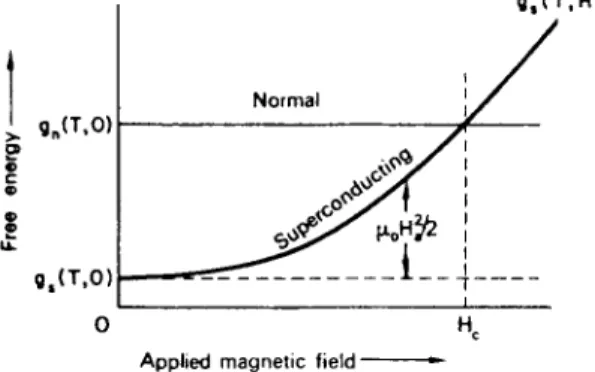
the transition t e m p e r a t u r e the free energy of the superconducting state must b e less than that of the normal state, otherwise the metal would re- main normal. Suppose that at a t e m p e r a t u r e T, and in the absence of an applied magnetic field (Ha = 0), the G i b b s free energy per unit volume of the superconducting state i s ^ ( T , 0) and that of the normal state isgn(T> 0) (Fig. 4.1). N o w let a magnetic field of strength Ha be applied parallel

, â , ( Ô , Ç )

Applie d magneti c fiel d ·-

FIG . 4.1. Effect of applie d magneti c field on Gibb s fre e energ y of norma l an d superconductin g states .

to the length of the rod. Any substance, which in an applied field Ha

acquires a magnetization / , changes its free energy per unit volume by an a m o u n t t

Ä£Çá) = -ì0 jldHa. (4.1)

0

So in the case of the field producing a positive magnetization, i.e. the magnetization in the same direction as the magnetic field, the free energy is lowered. [ N o t e that (4.1) implies that, w h e n a substance is magnetized by an applied magnetic field, its free energy changes b y an a m o u n t proportional to the area under its magnetization curve (/ v. Ha). T h i s is a useful general result, which w e shall employ several times.] In t h e case of a superconducting specimen the application of a magnetic field produces a negative magnetization which, if penetration of the field is neglected, exactly cancels the flux due to the applied field, so that / = — H. T h e free energy per unit volume is therefore increased to

gs(T,H) = gs(T,0) + ì0^ \I\dHa. ï

t See Appendi x B.

In fact 11\ = H, so the magnetic field raises the free energy density to

ÅëÔ,Ç) = 8é{Ô,0) + ì 0 ø . ( 4 . 2 )

So, when we apply a magnetic field to a superconductor, its free energy increases to this value due to the magnetization (Fig. 4 . 1 ) . T h e normal state, however, is virtually non-magnetic and acquires negligible magnetization in an applied magnetic field. Consequently the application of a magnetic field does not change the free energy of the normal state though it raises that of the superconducting state. If the field strength is increased enough, the free energy of the superconducting state will be raised above that of the normal state, and, in this case, the metal will not remain superconducting but will become normal. T h i s occurs when gs(T> H) > gn(T, 0 ) , which with ( 4 . 2 ) gives

Ë | > [ ^ 0 ) - & ( Ã , 0 ) ] ,

T h e r e is therefore a m a x i m u m magnetic field strength that can b e applied to a superconductor if it is to remain in the superconducting state. T h i s critical magnetic field strength is given by

HC{T) = [g„(T, 0 ) - gs(T, 0 ) ] } \ ( 4 . 3 ) T h i s critical magnetic field which w e have derived b y a thermodynamic

argument is the same as the critical field which we discussed on p. 4 0 in terms of a critical current density.

T h e critical magnetic field strength can be measured quite simply by applying a magnetic field parallel to a wire of superconductor and observ- ing the strength at which resistance appears.

4.2. Variatio n o f Critica l F i e l d w i t h T e m p e r a t u r e If the critical magnetic field of a superconductor is measured, its value is found to depend on the temperature (Fig. 4 . 2 ) , falling from some value H0, at very low temperatures, to zero at the superconducting transition temperature Tc. A diagram such as Fig. 4 . 2 can be called the phase diagram of a superconductor. T h e metal will be superconducting for any combination of temperature and applied field which gives a point, such as P , lying within the shaded region. As the arrows indicate, the metal can be driven into the normal state by increasing either the temperature or the applied field, or both.

Temperatur e +-

FIG . 4.2. Phas e diagra m of a superconductor , showing variatio n with temperatur e of the critica l magneti c field.

0 1 2 3 4 5 6 7 8

Temperatur e (°K)

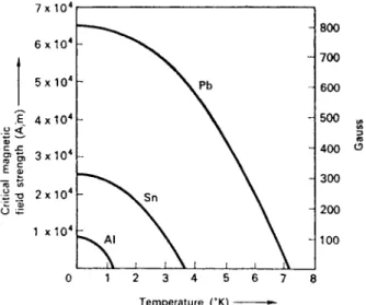
FIG . 4.3. Critica l fields of some superconductors .

T h e value of HQ is different for each superconducting metal; metals with low transition temperatures have low critical fields at absolute zero.

So each superconductor h a s a different phase diagram (Fig. 4.3). F r o m experiment it h a s been found that t h e critical fields fall off almost as t h e square of t h e temperature, so t h e critical field curves are closely a p - proximated b y parabolas of t h e form

7 x 1 0⁴ • 6 x 1 0⁴ - 5 x 1 0⁴ - 4 x t 0⁴ - 3 x 1 0⁴ - 2 x 1 0⁴ -

1 ÷ 10⁴ ;

800 700 600 500 „

(A 3

400 5 300 200 100

H

C

= H

0

[\-(T/T

c

n

(4.4) where H0 is the critical field at absolute zero and Tc is the transition temperature. E a c h superconductor can be characterized by its particular values of H0 and Tc, and, knowing these, we can use (4.4) to find the critical field at any temperature. T a b l e 1.1 lists values of H0 and Tc for the superconducting elements.

W e may remark here that there is no fundamental significance in the relation between critical field and temperature being a parabola. It has merely been found experimentally that the variation can b e conveniently described to within a few per cent by a parabolic curve. T h e experimen- tal curves are not in fact exactly parabolas, and to describe t h e m ac- curately one would need a polynomial expression. For most calculations, however, it is sufficient to use the parabola given by (4.4).

The Cryotron

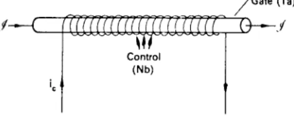
T h e existence of a critical magnetic field has been m a d e use of in a controlled switch called a cryotron (Fig. 4.4). T h e current J which is to be controlled flows along a straight wire of tantalum called the " g a t e " .

Around this, but insulated from it, is a niobium wire wound in a long single-layer coil called the "control". W h e n cooled to 4-2°K by immer- sion in liquid helium both the tantalum gate and the niobium control are superconducting, and the gate offers no resistance to the passage of the current / . If, however, a current ic is passed through the control coil, it generates a magnetic field along the gate, and, if the control current is large enough, the gate is driven normal by the magnetic field, and the appearance of resistance reduces the current , / . T h e control coil, however, remains resistanceless because the critical field of niobium is considerably higher than that of tantalum. Hence the current J through the gate can be controlled by a smaller current in the control, and the

Gat e (Ta )

Contro l (Nb )

•e

FIG. 4.4. Cryotron of tantalum and niobium.

device is analogous to a relay. Small cryotrons were first developed as fast acting switches for possible use in digital computers. L a r g e cryotrons can b e used to control the currents in superconducting magnet circuits (see § 1.3).

4.3. M a g n e t i z a t i o n o f S u p e r c o n d u c t o r s

W e n o w discuss h o w the magnetization of a superconducting specimen varies as a magnetic field of increasing strength is applied. L e t us again consider a rod of superconductor and imagine a magnetic field Ha to b e applied parallel to its length. Figure 4.5a shows how the flux density  inside the specimen varies as w e increase the strength of the

Superconducto r

I = Ï

(b ) FIG . 4.5. Magneti c behaviou r of a superconductor .

applied field. N o r m a l metals (excluding the special ferromagnetic metals, such as iron) are virtually non-magnetic and so the flux density  inside them is proportional to the strength of the applied field,  = ìïÇ á, as shown by the dotted line in Fig. 4.5 a. A superconductor, however, is perfectly diamagnetic if we neglect the penetration depth, and as t h e applied magnetic field strength is increased, the flux density within the specimen remains at zero. But when the applied field strength reaches the critical value Hc, the superconductor is driven into the normal state, and the flux due to the applied field is no longer cancelled inside. At all higher applied field strengths the superconductor behaves j u s t like a nor- mal metal. F o r a pure specimen this behaviour is reversible; if the applied magnetic field is decreased from a high value, the specimen goes back into the superconducting state at the value Hc and below this there is no net flux inside.

THE CRITICAL MAGNETIC FIELD

W e can describe the magnetic behaviour of a superconductor in another way. W e have seen that, when a metal is in the superconducting state, there is no magnetic flux inside, because surface currents circulate to give the specimen a magnetization J exactly equal and opposite to the applied field, so that / = — Ha. Figure 4.5b shows how the magnetization of a superconductor varies with the strength of the applied magnetic field. W h e n the applied field strength reaches Hc the superconductor becomes normal and the negative magnetization disappears. At higher applied fields the superconductor has, like any normal metal, virtually n o magnetization. Figure 4.5 is, of course, just t w o equivalent ways of presenting the same information. W e need t o be familiar with the form of b o t h curves, because sometimes it is convenient to consider the inter- nal flux density, whereas on other occasions it is more convenient to con- sider magnetization.

4 . 3 . 1 . " N o n - i d e a l " s p e c i m e n s

T h e magnetic properties w e have been considering so far in this chapter are those that would be shown by "ideal" specimens, i.e. those containing no impurities or crystalline faults. Any real specimen is, however, not perfect, and its behaviour will depart to some extent from the behaviour w e have just described. Nevertheless, it is possible with great care to produce specimens so nearly perfect that they have proper- ties very closely approximating to the ideal. However, the greater the degree of imperfection the greater will be the departure from ideal behaviour.

An ideal specimen has a sharply defined critical field strength and its magnetization curve is completely reversible. Figure 4.6 illustrates the

ï ^Ç

Ç

FIG . 4.6. Magneti c behaviou r of a non-idea l superconductor .

I.T.S.—c

magnetic behaviour of an imperfect sample. It can b e seen that there is no longer a sharply defined critical magnetic field, the transition from the superconducting t o normal state being "smeared o u t " over a range of applied field strengths. F u r t h e r m o r e , the magnetization is not reversible;

in decreasing fields the curves follow different p a t h s from those traced in the original increasing field. W e call this hysteresis. Finally, when the applied field h a s been reduced to zero, there m a y remain some positive magnetization of t h e sample, giving rise to a residual flux density BT and magnetization IT. W e say the sample h a s trapped flux. In this condition the superconductor is like a permanent magnet.

W e see, therefore, that a non-ideal specimen m a y show:

1. Ill-defined critical magnetic field.

2. Magnetic hysteresis.

3. T r a p p e d flux.

T h e s e three departures from ideal behaviour do not necessarily all occur together. F o r example, a specimen m a y not have a sharp critical field and may show hysteresis b u t still not trap any flux. Defects involving large n u m b e r s of atoms, such as particles of another substance or the chains of displaced a t o m s k n o w n as dislocations, tend to give rise to hysteresis and trapped flux, whereas impurity a t o m s and unevenness of composi- tion reduce the sharpness of the critical field. T h e reasons why different kinds of impurity and imperfection produce the various departures from ideal behaviour are complicated and not yet fully understood, and so w e shall not discuss t h e m in detail here. However, these effects are of con- siderable practical importance and w e shall return to them again in Chapter 12.

4 . 4 . M e a s u r e m e n t o f M a g n e t i c P r o p e r t i e s

T h e techniques which can be used to measure the magnetic characteristics of superconductors do not differ in principle from those used in m e a s u r e m e n t s on ordinary magnetic materials, such as a ferro- magnetics; b u t they must, of course, b e suitable for use at very low temperatures. T h e m e t h o d s fall into t w o classes: those which measure the flux density  in the sample and those which m e a s u r e the sample's magnetization / (Fig. 4.5). T h o u g h either of these gives the full informa- tion on the magnetic properties of the sample, it m a y be convenient to choose one or other m e t h o d of measurement, depending on cir- cumstance. M a n y different types of a p p a r a t u s have been used, of various

THE CRITICAL MAGNETIC FIELD

degrees of complexity depending on the sensitivity, degree of automa- tion, etc., required. However, these are all based on the simple methods we now describe.

4 . 4 . 1 . M e a s u r e m e n t o f flux d e n s i t y

T h i s is a very simple measurement which does not require any moving parts in the low temperature region. T h e principle is to measure the magnetic flux which appears in a specimen when a magnetic field is applied. O n the specimen X (Fig. 4.7) is wound a " p i c k - u p " coil C con- sisting of a few hundred t u r n s of fine wire. T h e ends of this coil are con- nected to a ballistic galvanometer G outside the low temperature ap- paratus. A magnetic field Ç can be applied parallel to the axis of the specimen by m e a n s of the solenoid S, and when the magnetic field is suddenly applied by closing the switch, the ballistic galvanometer will be deflected by an amount proportional to the flux threading the pick-up coil C, i.e. the deflection is proportional to the flux density B. Hence by successively applying stronger magnetic fields we can follow the varia-

D.C.

powe r suppl y

FIG . 4.7. Measuremen t of magneti c flux densit y in a superconductor .

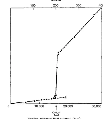
tion of  with field strength H. Figure 4.8 shows a  versus Ç characteristic obtained in this way. T h e critical field Hc at which the specimen ceases t o b e perfectly diamagnetic can clearly b e seen.

I n the case of a non-ideal specimen some flux will be trapped and so, when the field is switched off, there will be a smaller reverse deflection of

Oerste d

Å ï

ù

0 10,000 | 20,000 30,000 Critica l

field

Applie d magneti c fiel d strengt h (A/m )

FIG . 4.8. Experimenta l result s of ballisti c flux measuremen t on a superconducto r (tantalu m at 3 7°K). Th e smal l "background " deflectio n è' is du e to th e flux densit y produce d by th e applie d field in th e actua l wir e of th e pick-u p coil (afte r Rose-Innes) .

the galvanometer. It is therefore necessary to note the galvanometer deflection b o t h when switching on and w h e n switching off the applied magnetic field in order t o observe h o w m u c h flux is trapped.

4 . 4 . 2 . M e a s u r e m e n t o f m a g n e t i z a t i o n

In this method the specimen is moved into and out of a pick-up coil which is connected t o a ballistic galvanometer. T h e throw of the

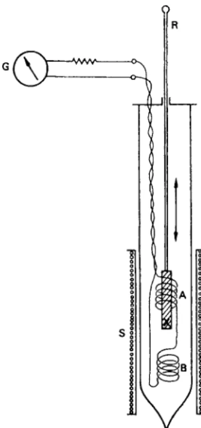
galvanometer will be proportional to the flux carried b y the sample and this will be proportional t o its magnetization. T h e method is illustrated in Fig. 4.9. T h e specimen X is mounted on the end of a sliding rod R so that it can b e moved from the upper pick-up coil A to the lower one B. A and  are identical coils, except that they are wound in opposite direc-

FIG . 4.9. Apparatu s to measur e magnetization .

tions. T o measure the magnetization of the sample a steady magnetic field of the required magnitude is applied by m e a n s of the solenoid S and the specimen is then moved quickly from coil A into coil B. In the case of a diamagnetic sample, the flux threading coil A will therefore increase and the flux through  will decrease. Since the t w o coils are connected in series opposition the e.m.f.s. induced in them will add together and the ballistic galvanometer will swing by an amount proportional to the magnetization of the sample. T h e measurement is repeated at gradually increasing applied magnetic field strengths, and so w e m a y construct a graph of sample magnetization as a function of applied field strength.

Because A and  are w o u n d in opposite directions any e.m.f.s. d u e to u n - intended fluctuations of t h e applied field strength should cancel and not deflect t h e galvanometer.

A feature of m e a s u r e m e n t s o n superconductors is that they are self- calibrating. At applied field strengths below t h e critical field strength, t h e slope of t h e / versus Ç curve always e q u a l s — 1 .

4 . 4 . 3 . I n t e g r a t i n g m e t h o d

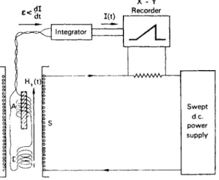
In this method, illustrated in Fig. 4.10, w e again have t w o identical pick-up coils A and  connected in series opposition, b u t t h e specimen is now permanently located in one of them. T h e current to t h e solenoid S is

÷ - Y

FIG . 4.10. Integratio n metho d of measurin g magnetization .

gradually and smoothly increased so that a continuously increasing magnetic field is applied t o t h e pick-up coils. An e.m.f. will b e developed across each coil, proportional t o t h e rate of change of t h e magnetic flux threading it, but, since one coil contains t h e sample and t h e other does not, and since they are in series opposition, t h e net e.m.f. 6 across t h e t w o coils will b e proportional t o t h e rate of change of magnetization of the sample:

T h i s e.m.f. is fed into an electronic integrator, a circuit whose output voltage is related to its input voltage by Voxxt oc j Vin dt. T h e output of the integrator is therefore

so at any time the output voltage of the integrator is proportional to the magnetization of the sample.

T h i s method of measuring magnetization h a s the advantage that no movement of the specimen is required, but the electronic equipment is more complicated than the apparatus described in the previous t w o sections.

ï