CHAPTER FIFTEEN KINETICS OF REACTIONS IN SOLUTION

CHAPTER FIFTEEN

KINETICS OF

REACTIONS IN SOLUTION

Much of the material of Chapter 14 is needed as a foundation for this chapter.

Particularly important are the sections on reaction rate laws, the relationship between reaction mechanism and rate law, and the collision and transition-state theories. We proceed to consider some aspects of rate laws that were omitted before and which are often encountered in solution kinetics, as well as experimental approaches that are now more relevant. Collision and transition-state theories are discussed again in terms of their special applications to solutions, and the main portion of the chapter concludes with a discussion of a number of types of reaction mechanisms.

The flavor of this chapter differs noticeably from that of Chapter 14. There is less emphasis on detailed, quantitative theories and more on reaction mechanisms.

One reason lies in the far greater variety of reactions in solution than in the gas phase. There are perhaps 30 important types of gas-phase reactions as compared to 1000 or more in solution. Gas-phase reactions are restricted to small (volatile) molecules and ions. Solution studies extend to protein and other macromolecular species. Reactions involving ions are a specialty in the gas phase, but dominate large areas of kinetics in solution.

An important and recurring theme, again special to this chapter, will be that of the role of solvent. The solvent affects the manner in which reacting molecules can come together and, further, it not only may specifically alter the structure or other properties of the reactants but often is itself a reactant. In fact, one of the difficulties of solution kinetics is the distinction between solvent as a medium and solvent as a direct participant in a rate-controlling step. Mechanistic schemes involving solvent are for this reason often more difficult to establish and more subject to controversy than gas-phase reactions, hence the relatively high degree of preoccupation with them by solution kineticists.

603

15-1 Additional Comments on Rate Laws. Reversible Reactions

It will be recalled that in Section 14-2 a detailed presentation was made of the mathematical behavior of first- and second-order rate laws. Some minor additional types of rate laws were mentioned, and the stationary-state hypothesis was developed in detail.

All of these treatments assume that the reaction goes to completion. It is entirely possible, however, for the equilibrium constant to be such that equilibrium is reached before the reactants are entirely consumed. In effect this means that the back reaction must be included in the rate equation. Although this situation can, of course, occur with either gas- or solution-phase reactions, it is perhaps more often encountered in the latter case; its consideration is therefore appropriate at this point.

A. Reversible First-Order Reaction

Consider the reaction

A + o t h e r r e a c t a n t s ^ Β + o t h e r p r o d u c t s , (15-1)

k²

where we suppose either that A is actually the only reactant and Β the only product or that the concentrations of other reactants and products are kept constant.

In either case, we take the consequence to be that the forward rate is first order in A and the reverse rate first order in B. If, as in Section 14-2A, only the forward reaction is considered, then the rate equation is

Rt = - ^ • = A r¹( A ) [Eq.(14-4)]

and, on integration, we obtain

(A) = (A)⁰ [Eq. (14-7)],

where (A)⁰ is the initial concentration, with the half-life t^1/2 given by M i/ 2 = 0.693 [Eq. (14-9)].

The reaction thus goes to completion; (A) approaches zero as t —• oo.

We next allow the reverse reaction to be significant, so that if one starts with no Β present, Ri is at first large but decreases as A is consumed, and Rh , zero initially, gradually increases as Β is formed. The net rate of reaction at any time is thus

^ = -^kl(A) + k²(B) (15-2)

or, since (B) = (A)⁰ — (A), d(A)

dt = - ^ ( A ) + k²[(A)⁰ - (A)].

15-1 ADDITIONAL COMMENTS ON RATE LAWS. REVERSIBLE REACTIONS 605

Separation of the variables leads to d(A)

k²(A)⁰ - (k, + k²)(A)

which gives, on integration, 1

= dt,

k + k L N^ 2( A )0 — {kx + k2)(A)] = t + constant.

On setting (A) = (A)⁰ at t = 0, we obtain

A^j^-ik. + k.e-"'),

where k = k^x + k². Equation (15-3) may be put in a more elegant form as follows.

At r = oo we have equilibrium, so that d(A)jdt = 0, and Eq. (15-2) gives K = ^ = (B)o°

k² (A) a ,

or, since (B)^ = (A)⁰ — (A)*, , rearrangement yields

( Α )^β 1 k²

(A)⁰ 1 + Κ k, + k²' (15-4)

where AT is the mass action law equilibrium constant. Since (A)⁰ k²\(k^x + k²) = (A)*, and (A)⁰ M * ! + = (A)⁰{1 - [kj(ki + h)]} = ( A )⁰ - ( Α )^β , Eq. (15-3) becomes

(A) (A)oo kt _

(A)⁰ — (Α)» * U > : > J

It follows from Eq. (14-35) that if & is any additive property, then UP

_

<S ^ o o - k t

Two alternative forms of Eq. (15-5) are

(A) ! , i/„-kt

= e-^kt. (15-6)

(A), and

1 + to"*' (15-7)

(A) _ 1 , Κ „.^kt

(A)⁰ 1 + Κ ¹ 1 + Κ or

+ ^-pe~^k\ (15-8)

(A)⁰ i + # ^ i + # '

Equation (15-5) makes clear the point that the rate law will still be first order in nature, provided that the quantity (A) — (A)*, is used rather than just (A).

Thus a plot of ln[(A) — (A)*,] versus t will be a straight line of slope — k. The

usual half-life relationships are obeyed, with kt^1/2 = 0.693. Notice, however, that the observed rate constant is k and not k^x. The experimental rate data thus give k = k^x + k², and (A)oo/(A)⁰ = k²l(k^x + k²), and these two pieces of informa­

tion allow k^x and k² to be calculated separately. If the reaction goes to completion, so that (A)oo = 0 and k² <^ k^x, Eq. (15-5) reduces to Eq. (14-6).

Example. T h e reaction

C H⁸B r + I " ft C H⁸I + B r "

is followed in a solvent in which K I and K B r are n o t very soluble. B y having excess solid I d and K B r present, the I~ and B r " concentrations are fixed a n d the forward and reverse reactions b e c o m e p s e u d o first order; k^x and k² are these first-order rate constants. In a particular experi­

ment there is initially 100% C H³B r ; the percentage drops t o 9 0 , 71.7, and 4 0 after 10 m i n , 35 m i n , and at equilibrium, respectively. Find k^x and k².

W e can verify that the reaction is a reversible first-order o n e by calculating k ( = f c i + k²) for the 10-min and 35-min points. T h u s k = - l n [ ( 9 0 - 40)/(100 - 40)]/10 = 1.82 χ 1 0 "² m i n "¹ and A: = - l n [ ( 7 1 . 7 - 40)/(100 - 40)]/35 = 1.82 x 1 0 "² m i n "¹. T h e constancy of A: s h o w s that Eq. (15-5) is obeyed. F r o m the equilibrium d a t u m , Κ = ( C H⁸I ) / ( C H⁸B r ) = 6 0 / 4 0 = 1.5.

Since Κ = kjk², w e find k² = 1.82 x 1 0 ~²/ 2 . 5 = 0.728 x 1 0 "⁸ m i n "¹ a n d k^x = \.5k² = 1.09 x 1 0 "8 m i n "1.

The set of curves shown in Fig. 15-1 is calculated from the alternative equation (15-9), which brings out more explicitly the effect of allowing the back reaction to assume increasing importance. As ^decreases from infinity, (A)/(A)⁰ approaches a larger and larger limiting (A)oo/(A)⁰ value, and the approach, while always exponential, is increasingly rapid. That is, although the initial rates are all the same, the back reaction comes in earlier and earlier to cause (A)/(A)⁰ to level off at the equilibrium value.

Similar but more complex analyses can be made for cases where either the forward or the reverse reaction is second order or where both are. Some of these are given in the Special Topics section. However, such treatments are difficult to use and to fit accurately to data, and it is good practice to try to establish experimental conditions such that the rate law is made pseudo first order.

I ι ι ι

0 1 2 3

kt

FIG. 1 5 - 1 . Rate of approach to equilibrium for the case A ^ B , for varying K. For Κ = 0 . 1 , ( A ) . / ( A ) o = 0.91 ;K = h ( A )^e/ ( A )⁰ = f , Κ = 2, ( Α )^β/ ( Α )^β = i ; Κ = α > , ( Α )^β/ ( Α )⁰ = 0.

15-1 ADDITIONAL COMMENTS ON RATE LAWS. REVERSIBLE REACTIONS 607 B. Kinetics of a Small Perturbation from Equilibrium

An important type of method for studying fast reactions, discussed in Sec­

tion 15-2B, consists in making a sudden change in the physical state of a system at equilibrium, such as a sudden j u m p in temperature, so that a different equilibrium constant applies and the system seeks its new equilibrium state. If the perturbation is relatively small, then the kinetics of this relaxation to the new equilibrium position takes on a rather simple mathematical form.

While the treatment may be generalized, it is best illustrated in terms of a specific example. Consider the dissociation of a weak acid

Η Α * ^ Η + + Α - , Κ' = Ρ±-, (15-10)

with (H+) = ( A^-) = Xe and (HA) = a — x^e' initially, where a is the total for­

mality of the acid present. As a result of a sudden temperature j u m p , the equi­

librium constant takes on a new value K, where Κ = k^x\k_^x, for which the corre­

sponding equilibrium concentrations are x^e and a — x^e, so that the system has been displaced from equilibrium by Δχ⁰ = x^e' — x^e. Net reaction will now occur with χ at some subsequent time t equal to x^e + Δχ. If the reaction is a simple one, that is, if Eq. (15-10) is also the mechanism for the reaction, then the reaction will take place according to the mass action rate law:

dx

~dt or

d(Ax) dt d(Ax)

dt

Since x^e is the new equilibrium value, it must be true that ki(a — Xe) = k_iXe2,

= k^x(a — x) — k_^xx²

= kx(a — Xe — Ax) — k_x(xe + Ax)2,

= k^x(a - Xe) - k^x A x - k_^xXe² — 2k_^xXe Ax — k^Ax)². (15-11)

so Eq. (15-11) reduces to d(Ax)

dt ^{= - kx Ax - 2k_x}xe Ax - k.^Ax)2. (15-12) At this point the characteristic assumption is made that Ax is sufficiently small

that square or higher-power terms in Ax can be dropped. In the present case the result is

= + 2k_^lXe) Ax = -k^T Ax. (15-13)

Equation (15-13) is first order in Δχ and integrates to give

Ax = Ax⁰ e-^k*\ k^T = - , (15-14)

τ

where k^T , the relaxation rate constant, is often reported as its reciprocal τ , the relaxation time. From Eq. (15-13) we have

k^r = k^x + 2k_^lXe = * ! (l + Ijf). (15-15) Thus if Κ is known, k^x and k_^x may be calculated.

15-2 Experimental Methods

A. General

Most of the experimental techniques described in Section 14-3 are applicable to reactions in solution. The system may be quenched, either by cooling or by

F I G . 15-2. Dilatometer.

The general derivation is somewhat complicated, but the result is that regardless of mechanism or actual rate law, the dropping of all terms higher than first power in Ax leads to Eq. (15-14), where k^r will have some specific relationship to the actual rate constants and various equilibrium concentrations. If the mechanism is in doubt, the form of the rate law may be deduced from a study of the variation of k^T (or of r) with system composition.

Example. A 0.010 / s o l u t i o n o f N H4O H experiences a sudden temperature j u m p terminating at 2 5 ° C , at which temperature # = 1 . 8 x 1 0 "5 m o l e l i t e r- 1 for the equilibrium N H4O H = N H4 + 4 - O H " , s o that xe = 4.1 x 1 0 "4 M. T h e observed relaxation time is 1.09 χ 1 0 "7 sec, corresponding t o kr = 9.2 χ 1 0e s e c "1. F r o m Eq. (15-15) w e have

9.2 χ 1 0E

ν _ 2 χ 1 05 s e c- 1

1 1 + [(2)(4.1 χ 10"4)/(1.8 χ ΙΟ"5)]

and L j = 2 χ 105/1.8 χ 10"5 = 1.1 χ 1 01 0 liter m o l e "1 sec"1. N o t e h o w a knowledge of kx

has allowed the indirect determination of an extremely large k_x. If there were any doubt about the correct rate law, it could be verified that k^x and k_^x were in fact independent of the ammonia concentration used.

15-2 EXPERIMENTAL METHODS 609 removal of a catalyst, and then analyzed chemically. Or an additive property may be used such as optical density at a suitable wavelength. A technique special to solutions is that of following the change in volume; the partial molal volumes of the reactants and products generally will differ, with the consequence that the total volume of the solution will increase or decrease as the reaction proceeds.

The change is usually not large but can be followed accurately if the system is in a dilatometer, or essentially a flask capped with a capillary tube (see Fig. 15-2) and well thermostated. The level of the meniscus in the tube is then measured periodically with a traveling microscope. The method is often resorted to if, as in the case of polymerization reactions, no very characteristic optical density changes occur. Equation (15-38) was followed dilatometrically, for example.

One does not, however, follow solution reactions by means of pressure change at constant volume. In the case of liquids the pressure necessary to maintain constant volume in the face of even a small partial molal volume change would be quite large—large enough to affect the rate constant itself (see Special Topics section).

β. Fast Reaction Techniques

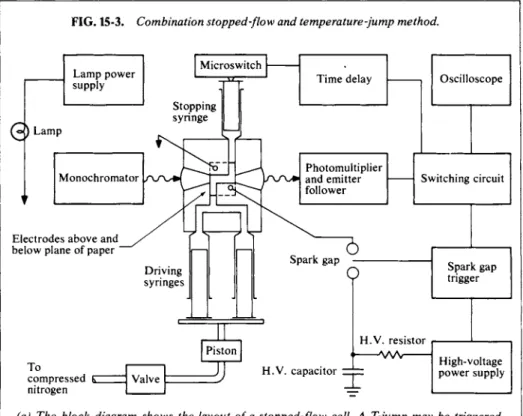
The types of methods just cited are applicable to reactions whose half times are 1 min or more. Reaction times as short as 0.1 sec can be investigated by means of rapid mixing devices such as illustrated in Fig. 14-5. The reacting solutions enter a mixing chamber and then travel down a small-bore tube; it is necessary that some color change arccompany the reaction so that the light absorption at a suitable wavelength can be used in the determination of the degree of reaction at various positions down the tube and hence for various times of reaction.

A number of additional methods have come into use in recent years which allow the time scale to be shortened considerably. An important one is called the stopped- flow method. Reacting solutions are again delivered into a mixing chamber, now

usually by means of motor-driven syringes. After an interval sufficient to establish a steady-state condition in the exit tube, the flow is stopped abruptly and the optical absorption is determined as a function of time thereafter. A schematic of such equipment is shown in Fig. 15-3(a); as indicated, the progress of the reaction, following stoppage of the flow, appears as a time trace on an oscilloscope. Reaction times of the order of milliseconds can be handled by this technique.

A different family of techniques is that known as relaxation methods. One starts with an equilibrium mixture and subjects it to some physical perturbation such that the system must adjust or relax to a new equilibrium condition. As shown in Section 15-IB, if the departure from equilibrium is small, the relaxation process will be first order even though the rate law is not. Various methods have been used to produce the perturbation, the most important one perhaps being the Γ- or temperature-jump method. The method is illustrated in Fig. 15-3(b) and some results in Fig. 15-3(c). By discharging a large condensor across electrodes placed in a conducting solution, one achieves a quick, ohmic heating. As a result of the temperature jump, the system is no longer in equilibrium, and one uses the usual monitoring light-oscilloscope technique to follow the rate of reequilibration.

FIG. 15-3. Combination stopped-flow and temperature-jump method.

L a m p p o w e r s u p p l y

M i c r o s w i t c h

Q) L a m p

S t o p p i n g syringe

M o n o c h r o m a t o r

T i m e d e l a y

E l e c t r o d e s a b o v e and b e l o w plane o f paper

P h o t o m u l t i p l i e r and emitter f o l l o w e r

D r i v i n g s y r i n g e s

Spark g a p

7 ) Q

T o

c o m p r e s s e d SI nitrogen

P i s t o n

V a l v e

37

O s c i l l o s c o p e

S w i t c h i n g circuit

Spark g a p trigger

H . V . resistor

H i g h - v o l t a g e p o w e r supply

(a) The block diagram shows the layout of a stopped-flow cell. A T-jump may be triggered after stopping of the flow, the cell then having electrodes and associated circuitry of the type shown in(b). [From J. E. Erman and G. G. Hammes, R e v . S c i . Instr. 37, 746(1966). ]

(b) The T-jump cell. The high voltage is ap­

plied across electrodes Β and C. Conical lenses D focus the monitoring light into the cell region and then recollimate it. The cell volume is only 0.2 cm³. [From "Investigation of Rates and Mechanisms of Reactions" (G.

G. Hammes, ed.), Wiley (Interscience), New York, 1974.]

The rate of ohmic heating is just dT/dt—

P-R/Cp V where C^P is the heat capacity of the solution in Jcm~³ Κ^Λ, and Vits volume in cm³. The current flow during the discharge of a condenser bank decays exponentially, how­

ever, i=(V⁰/R) e x p (-t/RC), where V⁰ is the initial voltage across the capacitor, R is the resistance, and C the capacitance. Combina­

tion of the two equations and integration gives

hT(t) = j^\i-^v-

\-

Typical ranges of values of the parameters are Vb, 10-100 kV; C, 0.01-0.1 μF; R, 20-200Ω;

and V, 0.1-25 cm³. The time constant RC/2 is thus 1-10 \isec and δΤ^ about 5°C.

C r o s s s e c t i o n

15-2 EXPERIMENTAL METHODS 611

A

1/11 M i l . J i l l 1111 M M t f ++• M M

J 1

(c)Some T-jump results. Oscilloscope tracing A shows the heating curve. The ordinate is in arbitrary absorbancy units and the abscissa scale is 10 μsec per division. Curve Β shows the Co(II)-diglycine reaction (abscissa scale 500 μsec per division). [From "Investigation of Rates and Mechanisms of Reactions" (G. G.

Hammes, ed.), Wiley (Interscience), New York, 1974.]

FIG. 15-3 (continued).

An interesting further development combines the stopped-flow and T-jump methods. The stopped-flow procedure yields a steady-state set of concentrations of reaction intermediates—one that changes relatively slowly (over milliseconds) after the flow is stopped. Immediately after the flow is stopped, an electrical discharge is triggered to produce the T-jump by means of the usual ohmic heating effect, and one may now observe the relaxation of the pseudo steady state.

A n o t h e r type o f relaxation m e t h o d m a k e s use o f s o u n d waves. T h e absorption o f s o u n d by a m e d i u m is a consequence o f various irreversible, essentially frictional processes that take place during the compression-rarefaction cycles that occur as a s o u n d wave passes through the solu­

tion. If a chemical reaction system is present, its position o f equilibrium is cyclically perturbed by the s o u n d wave, with the frequency o f the sound. If the rate of reaction is slow, then the chemical system c a n n o t follow the changing equilibrium constant, and the solution behaves simply as a nonreacting mixture o f solutes. If the reaction rate is fast c o m p a r e d t o the s o u n d frequency, then the reacting system does follow the changing equilibrium position, with the result that energy is taken from the s o u n d w a v e t o supply the heat of reaction; the absorption coefficient or rate o f attenuation of the s o u n d w a v e is thereby increased. T h e transition between the t w o extremes o f n o effect and m a x i m u m effect occurs fairly narrowly at a frequency corres­

p o n d i n g to the relaxation t i m e o f the chemical system. T h e variation in the absorption c o ­ efficient o f the s o u n d with its f r e q u e n c y — k n o w n as the dispersion curve—has a n inflection point at the frequency equal t o l / τ , where τ is the relaxation time as given by Eq. (15-14). B y using high-frequency s o u n d , o n e can observe reaction times o f as short as perhaps 10 microseconds.

Reactive species may also be generated photochemically (see Section 19-4D) on a microsecond time scale by conventional flash photolysis, and in nanosecond and even picosecond times using a pulsed laser. Very fast subsequent reactions can be studied by using a monitoring beam and the photomultiplier-oscilloscope detection technique. The same is true in pulse radiolysis experiments, in which the reactive species are formed by means of a very short burst of electrons or of other high- energy radiation.

15-3 Kinetic-Molecular Picture of Reactions in Solution

A. Encounters

The physical picture of molecular motions in a liquid is rather different from that in a gas. The molecules of a liquid are about as close together as in the crystalline solid—there is usually about a 10% expansion on melting (water being an exception because of its unusually open crystal structure) which allows some looseness and randomness in the liquid structure. As illustrated in Fig. 8-7(b), it seems likely that molecules of a liquid are in a potential well, but a somewhat flattened one so that vibrations against immediate neighbors are of low energy.

There is, nonetheless, a confinement which is usually referred to as the solvent cage effect. The physical picture is then one of a molecule vibrating a number of times against the walls of its cage, that is, against its immediate neighbors, with occasional escapes to some adjacent position. The situation is illustrated in Fig. 15-4, where the molecules are shown as roughly spherical and in a somewhat expanded but essentially close-packed arrangement.

The cage model is supported by the fairly successful treatment of diffusion in liquids (see Section 10-ST-2) in which the random diffusional motion of molecules in a liquid is taken to occur as a sequence of jumps from one molecular position to the next. This elementary j u m p distance λ is about 2r, where r is the radius of the molecule. By Eq. (2-67),

# = (15-16)

ZT

The average time between jumps should then be

r = 05-17)

Equation (2-67) assumes a continuous medium, and since we are treating a liquid as having a quasi-crystalline structure, with more or less definite molecular sites, it turns out that a somewhat more accurate statement should be

λ² λ²

^ = 6 ΐ

= 6 H r

"

For small molecules a reasonable value of λ is about 4 A, and, from Table 10-4, 2 at 25°C would be about 1 χ 10~⁵ cm² sec-¹; τ is then about (4 χ 10"⁸)²/(6)(1 χ ΙΟ"⁵) ^ 2.5 χ 1 0 ~^η sec. We next guess that the solvent cage

FIG. 15-4. The solvent "cage.'

15-3 KINETIC-MOLECULAR PICTURE OF REACTIONS IN SOLUTION 613

F I G . 15-5. Diffusional encounter between A and B.

is sufficiently loose that the average vibrational energy is about kr, corresponding to a frequency hv = k r or ν = kT/h. Vibrations against the wall of the cage then occur at intervals of h/kT or about 1.5 χ 1 0^{- 1 3} sec at 25°C. We conclude that a typical molecule in solution vibrates about 2.5 χ 10~ⁿ/1.5 χ 10~^{1 3} or about 150 times against its immediate neighbors before escaping to a new position and new neighbors.

The same analysis applies to solute molecules, and the next task is to estimate the frequency with which two solute molecules A and Β will, by diffusion, accidentally become neighbors (Fig. 15-5). Such a process is called an encounter and the estimation of encounter frequencies is central to much of solution kinetics.

The problem is a difficult one, complicated by the present impossibility of describ­

ing the structure of a liquid with any great accuracy. As an approximation, we assume the molecules of solvent and of A and Β to be about the same size and to be spherical. Each A molecule should then have about 12 nearest neighbors, so that on each diffusional j u m p it should find 6 new ones. The chance that one of these will be a molecule of Β is given by the mole fraction of Β in the solution,

_ molecules of Β c m "³ _ n^B

*^{B —} molecules of solvent c m^{- 3} ~~

T / y X

"

where γ is a geometric factor which reflects the way in which molecules are packed in the liquid and λ³ is the molecular volume. Substitution into Eq. (15-18) gives the frequency 1/τ^{Α Β} of encounters of A with Β as

1 6!3

- i - = ^ - ( n^By A 3 ) ( 6 ) ^ 3 6 y A n^B^ .

TA B A

If we take the effective 2& to be the sum of @^A and @^B , γ to be about 0.7, and λ to be the sum of the molecular radii r^{A B} ,

— ~ 2 5 r^{A B}^^{A B}n^B. (15-20)

TA B .

The total number of encounters per cubic centimeter per second is this value multiplied by n^A or, in mole per liter units,

Z e ,^AB = 2 5 r A

i

^

° (A)(B), (15-21)

where Z^{e > A B} is the A - B encounter frequency. The corresponding frequency factor is

β. Application of Collision Theory to Reactions in Solution

It would seem that collision theory, based on the kinetic molecular theory of gases, would be totally inapplicable to reactions in solution. The surprising and very significant fact is that a number of solution reactions do have an Arrhenius frequency factor A [Eq. (14-57)] which is close to that expected from collision theory ( ^ 5 χ 10^{1 1}). Some representative data are given in Table 15-1. In other cases, although the frequency factor may be smaller than the theoretical value, it is not affected by the nature of the medium, as illustrated by the data of Table 15-2. More qualitatively, a number of other reactions have been found to have the same rate in the gas phase as in solution; for example, the rate of decomposition of Ν²Ο^δ is about the same in the gas phase as in nitromethane solution.

These examples are ones in which there is probably not a great deal of specific interaction between the solvent and the reacting solutes, and it seems necessary to conclude that at least in such cases the bimolecular collision frequency is about the same as in the gas phase. This conclusion, incidentally, provides a qualitative rationale for the fact that the osmotic pressure equation (10-22) has the same form as the ideal gas law. The frequency of solute collision against the semipermeable membrane appears to be the same as for gaseous solute at the same volume and temperature, thus making the osmotic pressure equal to the corresponding gas-phase pressure.

We can also return to Fig. 8-7(b) for a rationalization of this conclusion. If the potential well has a flat bottom, the vibrations of a molecule against its neigh­

bors may be of low enough energy that there is an equipartition distribution

T A B L E 15-1. Some Second-Order Reactions in Solutions'¹

A E*

Reactants Solvent (liter m o l e^{- 1} s e c^{- 1}) (kcal m o l e^{- 1}) C H³B r + I - C H³O H 2.26 χ 1 0^{1 0} 18.25

H²0 1.68 χ 1 0^{1 0} 18.26

I² + N²C H C O O C²H⁵ CCI4 2.21 χ 1 0^{1 1} 20.23 C²H⁵B r + ( C²H⁵)²S Q H6C H2O H 1.40 χ 1 0^{1 1} 25.47

α See E. A . Moelwyn-Hughes, "Physical Chemistry," 2nd ed. Pergamon, Oxford, 1961.

For @^A = @^B = 1 χ ΙΟ"⁵ cm² sec"¹ and r^{A B} = 4 A, A^e = 1.2 χ 10⁹ liter mole"¹ s e c^{- 1}.

A very simple and useful approximation results if 2 is estimated by means of Eq. (10-42) so that r^{A B} cancels out. The result is

A^e = 1.1 x 1 0⁵— liter m o l e -¹ sec"¹. (15-23) V

In summary, for a solution 1 Μ in A and 1 Μ in Β the encounter frequency at 25°C is about 4 χ 10⁹ mole l i t e r "¹ s e c^{- 1}. Having made an encounter, A and Β remain in their solvent cage for some 150 vibrational periods. We next contrast this picture with that provided by gas collision theory.

15-3 KINETIC-MOLECULAR PICTURE OF REACTIONS IN SOLUTION 615 T A B L E 15-2. Dimerization of Cyclopentadiene ^a

log Λ E*

Medium (liters m o l e^{- 1} s e c^{- 1}) (kcal m o l e^{- 1})

G a s 6.1 16.7

C²H⁵O H 6.4 16.4

C S² 6.2 16.9

C^eH^e 6.1 16.4

α Source: S. W. Benson, ' T h e Foundations of Chemical Kinetics." McGraw-Hill, N e w York, 1960.

among vibrational states (note Section 8-CN-l). The degrees of freedom of such vibrations will then be rather like three degrees of translational freedom insofar as the frequency of intermolecular impacts is concerned. Thus if a molecule having a room-temperature gas-kinetic theory velocity of 4 χ 10⁴ cm s e c "¹ were simply bouncing back and forth in a box of about 4 A on the side, its collision frequency with the walls would be about 1 χ 1 0^{1 2} s e c^{- 1}, or about the same as the vibrational frequency kT/h.

C . Encounters versus Collisions

The previous discussion about encounters does tell us, however, that although the collision frequency may be the same in the gas phase and in solution, the pattern of collisions must be quite different. Consider the case of molecules A and Β both 1 Μ in concentration. The gas collision frequency at 25°C would be about 5 χ 1 0^{1 1} l i t e r "¹ s e c "¹ and, as illustrated in Fig. 15-6(a), if each A - B collision could be marked on a time scale, their pattern would be a random one.

The encounter frequency would be about 4 χ 10⁹ l i t e r "¹ s e c "¹, or 1/100 as often. The two molecules would stay in their mutual solvent cage for about 2.5 χ 1 0 "^{1 1} sec, however, or long enough to make about 100 collisions with each other. The collision pattern is therefore as shown in Fig. 15-6(b)—occasional encounters with many collisions during each encounter.

IHIIL

T i m e (a)

• ii

T i m e (b)

F I G . 15-6. (a) Pattern of A - B collisions according to collision theory and (b) pattern of A - B collisions according to encounter picture.

The activation energies cited in Table 15-1 are around 20 kcal m o l e^{- 1}, which means that at 25°C the chance of a collision leading to reaction is about exp(-20,000/298#) or about 1 0 "^{1 5}. Thus only after 1 0^{1 5} collisions, or 1 χ 1 0^{1 3} encounters, does reaction occur, on the average. The difference in pattern between Fig. 15-6(a) and Fig. 15-6(b) is thus unimportant in such cases. If, however, the acti­

vation energy is small so that reaction should occur after only a few collisions at the most, then every encounter should result in reaction. Further, the frequency factor for the reaction is now limited by the encounter frequency. Reactions which occur with every encounter are said to be diffusion-controlled. Their observed activation energy will not be zero, however, but will be determined by the tem­

perature dependence of @^{A B} [in Eq. (15-22)] and hence by that of the viscosity of the solvent since by Walden's rule (Section 10-7B), @η is approximately a constant. From Table 8-4, this means that diffusion- or encounter-controlled reactions should show activation energies of 3-4 kcal m o l e^{- 1} in common solvents.

Reactions of this type are discussed in somewhat more detail in the next section.

There is an aspect of the theoretical treatment of encounter frequencies that should be mentioned at this point. In deriving Eq. (15-21), we assumed that the distribution of A and of Β in solution was random. If we focus on A as the species making the encounter, the derivation also assumes that as A diffuses away after an encounter it remains available to make new encounters with the same or nearby Β molecules. If, however, chemical reaction takes place with every encounter, then Β acts as a sink into which A disappears and there is therefore on the average a depletion of A in the vicinity of Β (and vice versa, of course). A simple treatment given by Smoluchowski in 1917 applies ordinary diffusion theory to this situation.

By Fick's law [Eq. (2-65); see also Section 10-7B] the total flux of A flowing toward a Β molecule is

>-(---*•"*(•*!£•).·

-

where stf is the area of the spherical surface around Β at a distance r. We now assume a steady-state condition, that is, that dn^A/dr is independent of time, so that Eq. (15-24) has the form

dn^A _ J

dr ~ ~ 4πή@^Α and integrates to give

where β is a constant of integration. We then set n^A = 0 at r = r^AB and n^A = n^A° , the average concentration, at r = o o , which allows a to be evaluated. On solving for J, we obtain

J = - 4Τ Γ ΓΑ Β^ΑΠΑ 0. (15-25)

We allow for the diffusion of Β by using ^^{A B} instead of just @^A , and multiply by n^B° to get the total encounter frequency

Ze.AB = 4 τ τ τ^{Α Β}^^{Α Β}η^Αη^Β (15-26)

15-3 KINETIC-MOLECULAR PICTURE OF REACTIONS IN SOLUTION 617

(dropping the superscript degree as no longer necessary), or the frequency factor

A,

-

· 05-27)

The frequency factor as given by Eq. (15-27) is about half of that from Eq. (15-23), and although both derivations are approximate, this comparison is probably about right. That is, the encounter frequency for a diffusion-controlled reaction is about half that expected in the absence of reaction. [Note that Eq. (15-33) should be used if A and Β are ions.]

D . Collision Theory as Modified for Solution Reactions

There are two limiting situations. The first, treated earlier, is that in which reaction occurs o n every encounter, so that the rate constant is given by Eq. (15-27) and the activation energy is that for diffusion (see Section 15-4). The second is that in which the chemical activation energy is large enough that reaction occurs only after many encounters. Practically speaking, this means that E* should be more than about 10 kcal m o l e^{- 1}. It is this second situation to which collision theory seems to apply about equally well in gas and solution reactions. W e can write

k = AeZee-**!*¹; (15-28)

where A^e is the encounter frequency factor, and z^e is the number o f collisions that occur during a n encounter; A^ez^e is the total collision frequency, or A in the Arrhenius e q u a t i o n ,

k = Ae~^E*l^RT [Eq. (14-57)].

I n terms o f the preceding qualitative treatment, A^e is given by 3 6 y A ^ V⁰/ 1 0 0 0 and z^e (kTlfyr, where τ is the lifetime of the encounter. This last m a y be altered by the presence o f attractive or repulsive forces between A a n d B. In the formation o f [ A B ] the v a n der Waals forces o f attraction (see Section 8 - S T - l ) between A a n d Β will be balanced against t h o s e between A and solvent and Β and solvent, since solvent is displaced in forming [ A B ] ; the net effect could be either a repulsion or a n attraction. In addition, o f course, hydrogen b o n d i n g m a y be present.

If w is the work o f separating A from B, then Eq. (15-18) should n o w be

τ ( 1 5 - 2 9 )

If w is positive, the encounters will last longer and more collisions will occur during each one.

If w e think o f the encounter pair as a weak c o m p l e x , w e c a n write A + Β ^ A B where R^t, the forward rate, is A^e(A)(B) and R^h is ( 1/ τ) [ Α Β ] . T h e equilibrium constant, K^e, is thus A^er.

Substitution into Eq. (15-28) gives

k = —Kee-k T ^E*/^RT (15-30)

h

Ic = —^S%lR^e-H%lRT^e-^E*l^RT^ (15-31)

h

N o t e that if w is zero, Ke 6 / Cs, where Cs is the concentration o f solvent i n m o l e l i t e r "1.

15-4 Diffusion-Controlled Reactions

According to the treatment of the preceding section, a diffusion-controlled reaction should have a rate constant of around 10⁹ liter m o l e^{- 1} s e c^{- 1} at 25°C and show an activation energy corresponding to that for diffusion or for the solvent viscosity, namely of 3-4 kcal m o l e^{- 1} for ordinary solvents. An implied condition is that the chemical activation energy be small enough that the reaction occurs within the first 100 collisions.

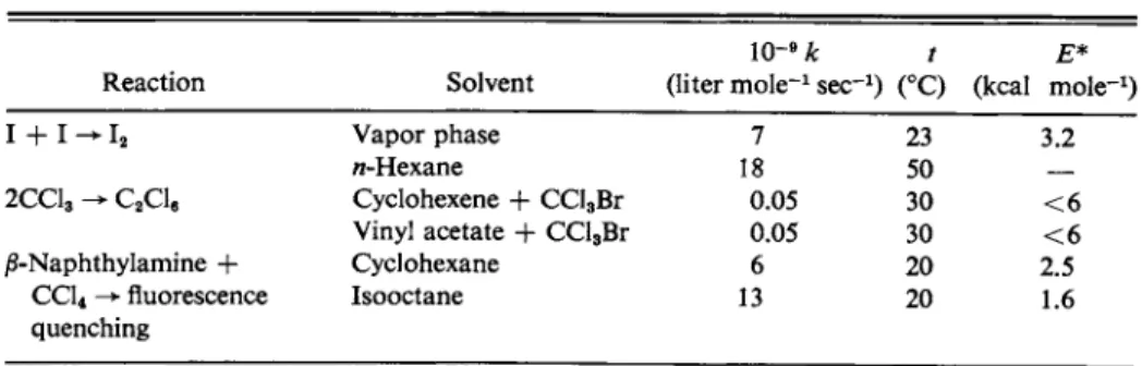
Some examples of what appear to be diffusion-controlled processes are given in Table 15-3. Note that the rate constants are around 10⁹ liter m o l e^{- 1} s e c^{- 1}, depending somewhat on the solvent and on the size of the reactants. Equally important, the activation energies are only a few kcal m o l e^{- 1}, or about that expected for diffusion in the solvents in question.

A number of acid-base type of reactions appear to be diffusion-controlled.

Table 15-4 gives the rate parameters for several reactions of the type

which are believed to be simple reactions, that is, the overall reaction also constitutes the mechanism. These reactions have been studied by one or another fast reaction techniques of the type mentioned in Section 15-2B. Notice that in all cases it is the back reaction, or the transfer of a proton from H³0 + to A^-, that is in the diffusion-controlled region of rate constant value; k^x for each forward reaction is then proportional to K, the equilibrium constant (see also Section 15-7).

The values of k² are distinctly larger than the 4 χ 10⁹ figure arrived at earlier for a diffusion-controlled reaction and at least two possible additional factors may be present over the usual situation. It will be recalled that the mobility of H+ ion is unusually large and that a Grotthus-type mechanism is presumably responsible.

As discussed in Section 12-5C, the hydrogen-bonded structure of water makes it possible for charge to move from one end of a chain of water molecules to the other by hydrogen bond shifts, the effect being the same as if a proton moved the length of the chain. It may then be that A " can acquire a proton from other than nearest-neighbor H³0⁺ molecules by means of a similar mechanism, so that A " and H³0⁺ do not have to diffuse as close to each other as in a normal bimolecu­

lar reaction. Their effective encounter rate would therefore be increased.

The second factor is that the reactants, being oppositely charged, experience

T A B L E 15-3. Some Diffusion-Controlled Reactions⁰

H A + H²0 ^ A " + H^sO⁺, (15-32)

Reaction Solvent

1 0 -⁹ k t £·*

(liter m o l e -¹ s e c -¹) (°C) (kcal mole"¹) I + I ^ I i Vapor phase

/i-Hexane

Cyclohexene + CCl³Br Vinyl acetate -f CCl³Br Cyclohexane

Isooctane

7 18

23 50 30 30 20 20

3.2

2CC1³ - C²C l^e 0.05

0.05

< 6

< 6 2.5 1.6 j8-Naphthylamine +

CC1⁴ fluorescence quenching

6 13

° Source: S. W. Benson, "The Foundations of Chemical Kinetics." McGraw-Hill, N e w York, 1960.

15-5 TRANSITION-STATE THEORY 619 T A B L E 1 5 - 4 . Fast Reactions of the Type

ΗΑ + Η²Ο ^ Α - + Η⁸0^{+ α}

H A pK& log k^x l o g Λ»

H²0 15.7^b - 4 . 6 11.1

H²S 7.0 3.9 10.9

H F 3.3 7.7 11.0 H S O r 1.6 9.4 11.0 CH3COOH 4.8 5.9 10.7

CH³COCH³ 2 0 - 9 . 3 10.7

( C H³)³N H + 9.8 1.0 10.8

j8-Naphthol^c 3.1 7.6 10.7

a Source: E. F . Caldin, "Fast Reactions in Solutions." Wiley, N e w York, 1964. T h e k values are in liter m o l e- 1 s e c- 1 at 25°C.

b K* has been put o n a basis consistent with other weak acids by writing it as (H+)(OH~)/(H20), that is, the usual value for has been divided by 55.5, the number o f moles o f H20 per liter.

c The reaction is o n e of deactivation of the first electronic excited state of 0-naphthol by proton transfer, as observed by fluorescence quenching.

an electrostatic attraction which enhances their diffusion toward each other.

It is a rather difficult problem to treat theoretically, but, qualitatively, the encounter frequency equation (15-27) is modified by an exponential term:

where φ should be proportional to z^Az^B , the algebraic product of the charges on the reactants. Since z^Az^B = — 1 in the present case, the exponential term acts to increase A^e over its normal value.

15-5 Transition-State Theory

The formal statement of transition-state theory is the same for solution as for gas-phase reactions. An elementary bimolecular reaction is given the intimate mechanism

A + Β = [AB]* [Eq. (14-79)], [AB]* ^ products [Eq. (14-80)],

where k^x = kT/h. The rate constant is then

kT „^t kT /AS°*\ (AH°*\ ^{r c n A Q M}

τ

h H

h * r - )

-

·

·

The equilibrium constant for forming the activated complex [AB]* or, alter­

natively, AS⁰* and AH⁰*, must reflect not only the changes in chemical bonding that occur but also any changes in solvation. As a consequence, the complete statistical mechanical evaluation of K* is too complicated to be of practical use

15-6 Linear Free Energy

Relationships. Reactions Involving an Acid or a Base

A. Acid-Base Systems

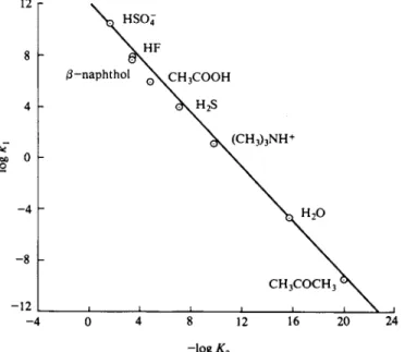
A rather interesting observation is that if some particular reaction is studied for a series of related compounds, then it will often be true that log k will vary linearly with log K, where k is the rate constant and Κ the equilibrium constant.

- 4 0 4 8 12 16 20 24 - l o g* a

FIG. 15-7. Data of Table 15-4 plotted according to the Br ousted equation (15-36).

in the case of solution systems. Portions of the partition functions can be estimated, however. For example, the translational entropy change can be calculated approxi­

mately from the change in the entropy of mixing accompanying Eq. (14-79) if ideal solutions are assumed. By Eq. (9-69), the entropy of mixing of a solution of A and Β for the standard state of 1 m is — (R In x^A + R In x^B) and that of 1 m [AB]*

is — R In X [ A B] * , where each mole fraction is just l/n^s, n^s being the number of moles of solvent per 1000 g. We are neglecting some change in entropy of the solvent, and on this basis

AstLns = ~ R LN * [ A B ] * + R In x^A + R In x^B = R In — . (15-34)

In the case of water n⁸ = 55.5, which gives ^S^t°^r*^{a i l s} = —4R and exp(AS°*/R) = 0.02.

This value, although obtained by a very different route, is essentially the same quantity as the purely statistical part of K^e of Eq. (15-30), which was found to be 6 / C^s, or about 0.1 for water.

Further aspects of the comparison between collision and transition-state theory as applied to solutions are taken up in the Commentary and Notes section.

15-6 LINEAR FREE ENERGY RELATIONSHIPS 621

a = - 1

12 16 2 0 - 2 0 - 1 6 - 1 2 - 8 - 4 0 4

l o g t f^a

F I G . 15-8. Bronstedplot showing both diffusion-controlled limits.

The actual relationship, proposed by Bronsted, is

or

k = (constant) AT^aa,

log k = b + a log K^&,

(15-35)

(15-36) where b and α are constants. The data of Table 15-4 for the reaction H A + H²0 - > A " + H³0⁺ are plotted in this manner in Fig. 15-7, and indeed, give a reasonably straight line, whose slope (and hence a) is 1.03. All this is rather misleading, however, since for these cases k² is essentially constant, being at the diffusion-controlled limit; and if k² is constant, then k^x must be proportional to Κ^Λ , so that on the log k^x versus log Κ^Λ plot a straight line of slope unity is auto­

matically expected. The more complete picture is as shown in Fig. 15-8. Thus k¹ should increase with Κ^Λ until the diffusion-controlled limit is reached and there­

after should be constant. Conversely, k² should increase with decreasing K& again until the diffusion-controlled limit is reached. When one k is at this limit, so that for it α = 0, then the other k must obey the Bronsted equation with a = 1. Thus oc varies from 0 to 1 (or —1) along each curve. The two curves need not be sym­

metric, although they have to cross at log Κ = 0. Also, there can be regions where neither k is at the diffusion limit, so that there can be an intermediate region for which both a's lie between zero and unity. It happened that the early studies on rates of dissociation lay in this intermediate region and that the range of values that was experimentally accessible was small enough that α appeared to be a characteristic constant for each acid.

Example. Estimate k¹ and k² for H^aC 0⁸ . T h e e q u a t i o n o f the line o f F i g . 15-7 is approxi­

mately l o g k^x = 11.7 + 1.03 l o g Κ^Λ . F r o m T a b l e 12-9, l o g Κ^Λ = - 6 . 3 7 , w h e n c e l o g k^x = 5.14 and k^x ^ 1.4 χ 1 0^δ s e c "¹. T h e n k² = KJk^x = 3.2 χ 1 0^{1 1} M "¹ s e c "¹.

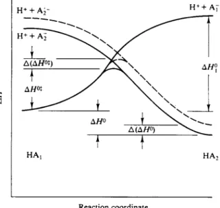
Equation (15-32) is merely a special case of an acid-base reaction

H A + B - = A " + H B .