Journal Pre-proof

(1)

Journal Pre-proof

Operator Splitting for Space-dependent Epidemic Model

Petra Csomós and Bálint Takács

PII: S0168-9274(20)30286-5

DOI: https://doi.org/10.1016/j.apnum.2020.09.010 Reference: APNUM 3935

To appear in: Applied Numerical Mathematics Received date: 3 December 2019

Revised date: 15 September 2020 Accepted date: 16 September 2020

Please cite this article as: P. Csomós, B. Takács, Operator Splitting for Space-dependent Epidemic Model,Applied Numerical Mathematics, doi:https://doi.org/10.1016/j.apnum.2020.09.010.

This is a PDF file of an article that has undergone enhancements after acceptance, such as the addition of a cover page and metadata, and formatting for readability, but it is not yet the definitive version of record. This version will undergo additional copyediting, typesetting and review before it is published in its final form, but we are providing this version to give early visibility of the article. Please note that, during the production process, errors may be discovered which could affect the content, and all legal disclaimers that apply to the journal pertain.

(2)

Operator Splitting for Space-dependent Epidemic Model

Petra Csomós, Bálint Takács

Institute of Mathematics, Eötvös Loránd University and MTA–ELTE Numerical Analysis and Large Network Research Group

Pázmány Péter sétány 1/C, H-1117 Budapest, Hungary

Abstract

We present and analyse numerical methods with operator splitting procedures, applied to an epidemic model which takes into account the space-dependence of the infection. We derive conditions on the time step, under which the numerical methods preserve the non- negativity and monotonicity properties of the exact solution. Our results are illustrated by numerical experiments.

1 Introduction

Epidemic modelling plays an increasingly important role not only in applied mathematics but also in medicine and public health. There is, for instance, a high demand on planning the right place and time of vaccination. The more complex these models are, the less hope we have in obtaining their analytical solution. Thus, the derivation and analysis of biologically adequate numerical methods means a vital challenge.

Epidemic models originate from the seminal work of Kermack and McKendrick [9] in 1927, who constructed a compartment model to study the process of epidemic propagation. The population is split into three classes: healthy but susceptible individuals, infected people who can infect other individuals, and already recovered or otherwise immune individuals. The first attempts describe two ways the individuals can “change” classes: (i) susceptible individuals get infected with some possibility, and (ii) infected people recover with some other rate of change.

There are several directions the original model can be generalised: by considering birth and death processes, by adding more classes of individuals, by considering a latent period, or, as in the present paper, by taking into account the effect of vaccination. In the present work we analyse an epidemic model which also treats the space-dependency of the effect of the infection, that is, the distance between the susceptible and infected individuals.

The novelty of our work is to apply operator splitting procedures when discretising in time. They allow us to split the model into two sub-problems, and solve them one after the other. With the help of operator splitting, the difficulty caused by the space-dependency can be handled separately. Moreover, the exact solution of the remaining part can be computed leading to a more stable and accurate numerical solution.

Since epidemic models describe real-life phenomena, it is vital to study whether they reflect the properties expected from the biological point of view. Therefore, we put an effort to investigate under which conditions the model’s numerical solution owns the non-negativity and monotonicity properties. We are also after the cases when our method gives higher bound on

(3)

the time step than the one already presented in the literature. We illustrate our theoretical results by numerical experiments.

Section 2 gives an overview on basic epidemic models and shows how we treat the space- dependency of infection. In Section 3 we introduce the space and time discretisation methods which are used later. In Section 4 we define the qualitative properties to be investigated in the rest of the paper. Section 5 contains some necessary technical tools. Sections 6, 7, and 8 are devoted to the analysis of the sequential, weighted, and Strang splitting, respectively. In Section 9 we present our numerical experiments illustrating the theoretical results. Section 10 briefly summarizes our results.

2 Space-dependent SIR model

Most of the currently used and analysed models are derived from the idea of Kermack and McK- endrick [9], who constructed the compartment model, introduced above, to study the process of epidemic propagation. LetS, I, R: R⁺0 →R⁺0 denote the density of susceptible, infected, and recovered individuals among the total population, respectively, and let the constant parameters a, b > 0 describe the rate of infection and recovery, respectively. Let S₀, I₀, R₀ ≥ 0 be given numbers. Then the susceptible–infected–recovered (SIR) epidemic model has the form







S⁰(t) =−aS(t)I(t), I⁰(t) =aS(t)I(t)−bI(t), R⁰(t) =bI(t)

(1)

for all t >0 with the initial condition

S(0) =S₀, I(0) =I₀, R(0) =R₀. (2)

The SIR model (1)–(2) is an initial value problem being a system of three ordinary differential equations. Although model (1) already describes several important features real epidemics posses, it does not take into account the spatial distribution of the different species, and sup- poses a homogeneous distribution on the domain. A model which considers the aforementioned properties was introduced by Kendall [8] in the following way.

For an arbitrary m ∈ N, we consider a bounded domain Ω ⊂R^m and the open ball B_δ(x) around the point x ∈ Ω with radius δ > 0. Let |B_δ(x)| denote its Lebesgue measure (or volume), and X_B_δ_(x)(t) the number of individuals in this ball for each X ∈ {S, I, R} at time t≥0. Then the density of class X at point x∈Ω and at timet >0 is defined as

X(t,e x) := lim

δ→0

1

|B_δ(x)|X_B_δ_(x)(t).

To ease the notation, we will omit the tilde, and denote the density by X(t,x) for each X ∈ {S, I, R}. The consideration above leads to a space-dependent SIR model which is, however, at this point not so beneficial because the density functions behave independently at each point x ∈ Ω. Since the infection takes place pointwise, it cannot spread in space, being however the main goal of the generalization. Thus, it is more natural to suppose that the infected individuals have an influence on the susceptibles in a certain distance around themselves in such a way that they less likely infect healthy individuals further away from themselves. That is, a susceptible can get infected only in a predefined domain, e.g., a circle. We note that the

(4)

radiusδ >0of the infectious domain can vary depending on the disease considered. We further suppose that the disease process is the same at every point x∈Ω.

Since it is the most common way, we also formulate our model in two-dimension and suppose a rectangular domainΩ = [0, A]×[0, B]⊂R² with some A, B >0arbitrary numbers (although the results of this paper can be extended to more general domains). Around the point x = (x, y) ∈ Ω, we denote the infectious domain by B_δ(x, y), being the circle with origin (x, y) and radius δ > 0. To this end, let r ≥ 0 denote an arbitrary point’s distance from (x, y) and ϑ ∈ [0,2π) its angle. The main idea is to replace I(t) in the terms ±S(t)I(t) in the space-dependent version of model (1) by the following weighted integral on the ball B_δ(x, y):

I(t, x, y) :=

Z ∞ 0

Z 2π 0

G(x, y, r, ϑ)I(t, x+rcos(ϑ), y+rsin(ϑ))rdϑdr (3) where function G: Ω×R⁺0 ×[0,2π) → R⁺0 describes the disease process in Ω. Since we aim at imitating the effect of an infected individual at the point (x, y) ∈ Ω on its δ-radius neigh- bourhoodB_δ(x, y), we want functionGto represent the combined effect of (i) the non-negative and monotonically decreasing function g₁: [0, δ]→R⁺0 which describes the dependence on the radius r, and (ii) the non-negative function g2: [0,2π) → R⁺0 describing the dependence on the angle. For the sake of simplicity, we build the infectious rate a > 0 into function g₁. We remark that the case of constant function g₂ is widely studied in [5] and [6]. A non-constant g2 may be useful for modelling the spread of diseases when there is a constant wind blowing in one direction which was described in [13]. We also suppose that the function g₂ is periodic in the way g₂(0) = lim

ϑ→2πg₂(ϑ). Since it is a natural assumption, we take the function G being separable in r and ϑ:

G(x, y, r, ϑ) =

(g1(r)g2(ϑ), if x+rcos(ϑ), y+rsin(ϑ)

∈Bδ(x, y),

0, otherwise. (4)

Then the term I in relation (3) has the following form:

I(t, x, y) = Z δ

0

Z 2π 0

g₁(r)g₂(ϑ)I(t, x+rcos(ϑ), y+rsin(ϑ))rdϑdr (5) for all t ≥0, (x, y)∈Ω.

To consider a more realistic model than (1), we take into account the effect of vaccination as well. Let c > 0 denote the rate related to the vaccinated population getting immune.

Then for the new unknown functions S, I, R: R⁺0 ×Ω → R⁺0, we get the following system of integro-differential equations:







∂_tS(t, x, y) = −S(t, x, y)I(t, x, y)−cS(t, x, y),

∂tI(t, x, y) = S(t, x, y)I(t, x, y)−bI(t, x, y),

∂_tR(t, x, y) = cS(t, x, y) +bI(t, x, y)

(6)

for all t ≥0, (x, y)∈Ω, and with the initial condition

S(0, x, y) = S₀(x, y), I(0, x, y) = I₀(x, y), R(0, x, y) =R₀(x, y), (7) where S₀, I₀, R₀: Ω→R⁺0 are given continuous functions such that

S₀(x, y) +I₀(x, y) +R₀(x, y)6= 0 holds for all (x, y)∈Ω. (8)

(5)

As already mentioned, one cannot hope to find an analytical solution to system (6), although it was proved in [14] that such a solution exists, which is also unique. Therefore, we are to use numerical methods to solve these equations. In the next section we introduce the space and time discretisation methods to be used in the present study.

3 Discretisation methods

The present section aims at introducing the space and time discretisation methods of the space- dependent SIR model (6) as well as the operator splitting procedures. Since it is the most challenging part of the numerical method being constructed, first we show how we approximate the integral appearing in (5).

3.1 Approximating the integral

The key point of the numerical solution of problem (6) is the approximation of the double integral in (5), which can be done in different ways. One approach is to approximate the function I(t, x+rcos(ϑ), y+rsin(ϑ)) by a Taylor expansion: the obtained method is studied in [5] and [6]. We note that this process is not efficient in the case of non-constant functiong₂ as shown in [13]. The other approach is to use a combination of interpolation and numerical integration (by using cubature formulas). For the present study we implement the second approach.

We consider a two dimensional cubature formula on the disc Bδ with positive coefficients.

For index set J ⊂ N² and for all (i, j) ∈ J, let r_i ∈ [0, δ] denote the (i, j)^th cubature points’

distance from the center point (x, y)∈Ω, and ϑ_j ∈[0,2π) its angle. Then Q(x, y) denotes the set of cubature points in the diskBδ(x, y)parametrized by polar coordinates (see [13] or [14]):

Q(x, y) =

x+ricos(ϑj), y+risin(ϑj)

∈IntBδ(x, y), (i, j)∈ J ,

where Int denotes the interior of the set. Numerical integration leads then to the following approximation of the term I(t, x, y) in (6):

T(t,Q(x, y)) = X

(i,j)∈J

w_i,jg₁(r_i)g₂(ϑ_j)I t, x+r_icos(ϑ_j), y+r_isin(ϑ_j)

(9) with some weights w_i,j ≥ 0. For the infected individuals being closer to the boundary of the domain Ω as the radius δ, the approximation of the integral in (5) needs values of I lying outside Ω: for these, we are going to use zero values. After these considerations we get the following system, being still continuous in t≥0 and (x, y)∈Ω:







∂_tS(t, x, y) = −S(t, x, y)T(t,Q(x, y))−cS(t, x, y),

∂_tI(t, x, y) = S(t, x, y)T(t,Q(x, y))−bI(t, x, y),

∂tR(t, x, y) = cS(t, x, y) +bI(t, x, y)

(10)

with the original initial condition (7). We note that there are several possibilities how to choose the quadratures. One can use a direct method which results in a uniform cubature, or transform the ball onto a square, and use generalised Gaussian quadratures on it. The results in [14] show that for less quadrature points, the uniform ones result in a smaller error, while for a denser quadrature, the non-uniform ones perform better. One can also compute the convolution in (5) by using the Fast Fourier Transform, which can be the direction of further research.

(6)

3.2 Spatial discretisation

In order to discretise problem (10) in space, we need a spatial grid G on the domain Ω = [0, A]×[0, B]. To this end we choose the arbitrary numbers K, L ∈ Z⁺ and define the grid resolutions h_x :=A/(K −1)>0 and h_y :=B/(L−1)>0 in directions x and y, respectively.

Then the grid itself is the following set:

G :=

(x_k, y_`)∈Ω|x_k= (k−1)h_x, y_` = (`−1)h_y, k = 1, . . . , K, `=, . . . , L . For all t≥0, (x_k, y_`)∈ G, and X ∈ {S, I, R}, we consider the approximate numbers

X_k,`(t)≈X(t, x_k, y_`) and T_k,`(t)≈T(t,Q(x_k, y_`)). (11) In order to determine the form ofT_k,`(t), we first projectI(t, x, y)to the gridG. Note that the points (x_k+r_icos(Θ_j), y_`+r_isin(Θ_j)) might not be part of the grid G, so we cannot assign any I_k,` values to them. Therefore, we approximate them by a bilinear interpolating method using the nearest knownI_k,` values and positive coefficients, resulting in the notation I. Thene we have

T_k,`(t) := X

(i,j)∈J

w_i,jf₁(r_i)f₂(Θ_j)I t, xe _k+r_icos(Θ_j), y_`+r_isin(Θ_j)

. (12)

It is worth mentioning that higher order interpolations, like cubic and spline, can be also used.

Although they do not preserve non-negativity, for a sufficiently small spatial grid resolution they behave as expected. It is also possible to use other, high order, non-negativity preserving methods, see [14]. We note here that if Ie≥ 0 holds, then Tk,`(t) is non-negative too, for all t ≥ 0 and (x_k, y_`) ∈ G. In order to ease the notation, we will leave the tilde throughout our computations.

3.3 Time discretisation

The main novelty of the paper is (besides the traditional time discretisation) that we use another time discretisation-like method: operator splitting. As one can see, the right-hand side of problem (10) can be written as a sum of two terms: one containing the integral and one with the remaining terms. The idea of operator splitting is to “split” the problem into two sub-problems with the corresponding terms alone, and solve them separately by using an appropriate initial condition to link their solution together. In the present paper we will introduce and study the sequential, the sequential weighted, and the Strang splitting schemes.

As already mentioned, it is natural to split the space-discretised SIR model (10) into the sub-problems with and without the integral term I specifying the space-dependency of the infection process:







∂_tS^[1](t, x, y) = −cS^[1](t, x, y),

∂_tI^[1](t, x, y) = −bI^[1](t, x, y),

∂_tR^[1](t, x, y) = bI^[1](t, x, y) +cS^[1](t, x, y)

(Sub.1) and







∂_tS^[2](t, x, y) = −S^[2](t, x, y)I^[2](t, x, y),

∂_tI^[2](t, x, y) = S^[2](t, x, y)I^[2](t, x, y),

∂_tR^[2](t, x, y) = 0

(Sub.2)

(7)

for all t≥0 and (x, y)∈Ω. The link between the sub-problems is the initial condition, as will be shown in the next sections.

For the later use we remark that sub-problem (Sub.1) can be solved exactly:







S^[1](t+τ, x, y) = e^−cτS^[1](t, x, y), I^[1](t+τ, x, y) = e^−bτI^[1](t, x, y),

R^[1](t+τ, x, y) =R^[1](t, x, y) + (1−e^−cτ)S^[1](t, x, y) + (1−e^−bτ)I^[1](t, x, y)

(13)

for all t ≥0 and (x, y)∈Ω, whereτ ≥0is an arbitrary time difference.

On the other hand, sub-problem (Sub.2) cannot be solved exactly. Its approximate solution can be obtained by another time discretisation method. For instance, the use of the first-order explicit Euler method with time step τ >0 leads to







S^[2]((n+ 1)τ, x, y) = S^[2](nτ, x, y)−τ S^[2](nτ, x, y)I^[2](nτ, x, y), I^[2]((n+ 1)τ, x, y) = I^[2](nτ, x, y) +τ S^[2](nτ, x, y)I^[2](nτ, x, y), R^[2]((n+ 1)τ, x, y) = R^[2](nτ, x, y)

(14)

for all n∈N with X^[2](0, x, y) = X₀(x, y) for each X ∈ {S, I, R}. We note that we take0∈N. The use of the second-order Heun’s method in Shu–Osher form (which preserves the strong stability, see [7]) with time step τ >0results in the following steps:











Sb^[2]((n+ 1)τ, x, y) = S^[2](nτ, x, y)−τ S^[2](nτ, x, y)I^[2](nτ, x, y), Ib^[2]((n+ 1)τ, x, y) = I^[2](nτ, x, y) +τ S^[2](nτ, x, y)I^[2](nτ, x, y), Rb^[2]((n+ 1)τ, x, y) = R^[2](nτ, x, y),

(15)











S^[2]((n+ 1)τ, x, y) = ¹₂S^[2](nτ, x, y)

+ ¹₂ Sb^[2]((n+ 1)τ, x, y)−τSb^[2]((n+ 1)τ, x, y)bI^[2](n+ 1)nτ, x, y) , I^[2]((n+ 1)τ, x, y) = ¹₂I^[2](nτ, x, y)

+ ¹₂ Ib^[2]((n+ 1)τ, x, y) +τ S^[2]((n+ 1)τ, x, y)I^[2]((n+ 1)τ, x, y) , R^[2]((n+ 1)τ, x, y) = ¹₂R^[2](nτ, x, y) + ¹₂Rb^[2]((n+ 1)τ, x, y) = R^[2](nτ, x, y).

(16) We do not plug formulae (15) into (16), because the method will be more suitable for analysis in its present form.

We note that the use of an additional time discretisation inside one time step might also lead to a non-negativity preserving method. This technique may be applied only for one sub- problem. Then the time step could be chosen independently of the constraints but related to the accuracy of the scheme. For more details on such kind of adaptive time stepping we refer to [4].

4 Qualitative properties

When combining the space and time discretisation methods presented in the previous section, we obtain a numerical method represented by a system of algebraic equations. By denoting

(8)

the approximation of X(nτ, xk, y`) by X_k,`ⁿ for all X ∈ {S, I, R}, the unknown values X_k,`ⁿ⁺¹ of these algebraic equations are computed with the help of X_k,`ⁿ for all n ∈ N, (x_k, y_`) ∈ G and X ∈ {S, I, R}.

In what follows we list several important properties which reflects real-life expectations. In the present work we will study whether the numerical solution possesses them.

1. By adding the equations of system (10), one obtain that the total size of the population remains constant in time at each space position:

∂_tS(t, x, y) +∂_tI(t, x, y) +∂_tR(t, x, y) = 0

S(t, x, y) +I(t, x, y) +R(t, x, y) =:C(x, y)for all t≥0 and (x, y)∈Ω. (17) This we expect from the numerical solution as well, i.e., that there exist numbers N_k,` such that:

S_k,`ⁿ +I_k,`ⁿ +Rⁿ_k,` =N_k,` for all n∈N, (x_k, y_`)∈ G. (P1) 2. Since functions S, I, R denote densities, their values should remain non-negative:

X(t, x, y)≥0 for all t≥0, (x, y)∈Ω and X ∈ {S, I, R}. (18) We expect the same from the numerical values as well:

X_k,`ⁿ ≥0 for all n∈N, (x_k, y_`)∈ G and X ∈ {S, I, R}. (P2) 3. Since infected or recovered individuals cannot be susceptible again, the function S is non-

increasing in time

S(t, x, y)≥S(t+τ, x, y) for all t, τ ≥0 and (x, y)∈Ω. (19) The same should hold for the numerical values as well:

S_k,`ⁿ ≥S_k,`ⁿ⁺¹ for all n∈N, (x_k, y_`)∈ G. (P3) 4. Similarly, the density of recovered individuals cannot decrease in time:

R(t, x, y)≤R(t+τ, x, y) for all t, τ ≥0 and (x, y)∈Ω. (20) Which means for the numerical values that

Rⁿ_k,`≤Rⁿ⁺¹_k,` for all n ∈N, (x_k, y_`)∈ G. (P4) In [14] it was shown that the properties (17)–(20) hold for the systems (6) and (10). So our aim is to construct such numerical methods which preserve their discrete versions (P1)–(P4).

(9)

5 Technical tools

Before the derivation and analysis of the methods, we collect some notations and technical tools we will use later on.

Notation 5.1. (i) For each X ∈ {S, I, R} we introduce the notation Xⁿ := ((X_k,`ⁿ )k=1,...,K,`=1,...,L)∈R^KL×KL.

(ii) LetM: R^KL×KL →R^KL×KLdenote the bounded linear operator (represented by a matrix in applications) that maps Iⁿ toTⁿ by the rule Tⁿ=M(Iⁿ). Furthermore, let

M :=kMk∞· kS⁰+I⁰+R⁰k∞

in which k.k∞ means the maximum matrix norm taken element-wise. We note that condition (8) implies M > 0.

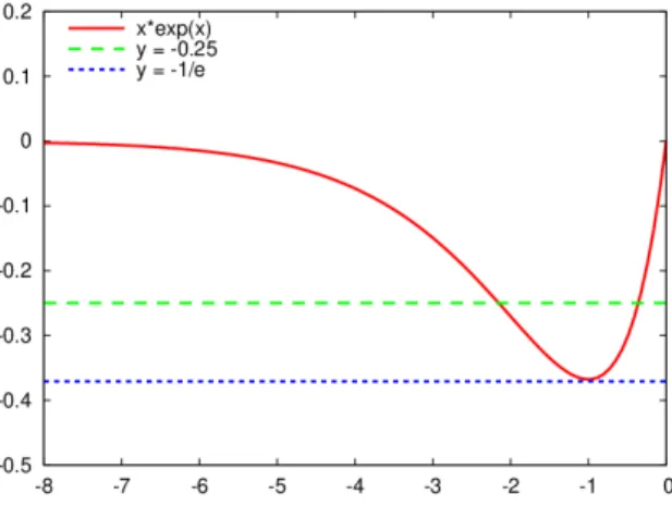
(iii) Let W₋₁: [−1/e,0) → (−∞,−1] and W₀: (−1/e,+∞) → (−1,+∞) denote the two branches of the Lambert-W function, that is, the inverse of the mapx7→xe^x.

(iv) For arbitrary p, q >0, we define the set T^p,q :=

0,−¹_pW0 − ^p_q

∪

− ¹_pW−1 − ^p_q ,+∞

⊂R. Furthermore, we define

T^0,q := [0,¹_q)⊂R.

The latter notation makes sense because of the following consideration.

Lemma 5.2. With Notation 5.1, the limit −¹_pW₀ − ^p_q ^p→0

−−→ ¹_q holds for arbitrary q >0.

Proof. It suffices to show that W₀(x)/x −−→^x→0 1 for x = −p/q < 0. The L’Hospital rule, the derivative of the inverse function, and the identity W0(0) = 0 imply that

x→0lim

W₀(x)

x = lim

x→0W₀⁰(x) = lim

x→0

1

e^W⁰^(x)+W0(x)e^W⁰^(x) = 1.

Remark 5.3. Since we will use it several times throughout the paper, we analyse the solution x <0to equation

xe^x =µ (21)

for some parameter µ <0.

(i) For µ <−1/e, there is no solution to equation (21).

(ii) For µ=−1/e, there is one solution: x1 =−1.

(iii) For µ >−1/e, there are two solutions: x−1 =W−1(µ) and x₀ =W₀(µ).

We also know that x−1 ≤x1 =−1< x0. Hence, for the inequality

xe^x ≥µ (22)

we have the following cases.

(10)

Figure 1: Graph of function x7→ xe^x. The horizontal lines indicate the µ-values −0.25 and−1/e.

(i) For µ <−1/e, the inequality (22) holds for every x <0.

(ii) For µ=−1/e, the inequality (22) holds for every x <0(we have xe^x =µfor x=−1).

(iii) For µ >−1/e, we have: x < x−1 =W−1(µ) orx > x₀ =W−1(µ).

The graph of function x7→xe^x is depicted on Figure 1.

In the next sections we will present the condition on the time step τ under which the qualitative properties (P1)–(P4) hold for the various operator splitting schemes. We are especially interested in the cases when the application of operator splitting leads to less severe condition than the one obtained without splitting. In [13] the authors applied the same space discretisation as showed in Section 3.2 and the explicit Euler method for the whole system (6) without taking into account the vaccination (c= 0). They found that property (P1) was automatically satisfied, and properties (P2)–(P4) held true for time stepsτ satisfying

τ ≤min 1

M,1 b

.

The case c >0 was studied in [14], and resulted in a similar bound, namely τ ≤minn 1

M +c,1 b

o

. (23)

From now on, the upper bound (23) will be considered as a reference value, and we will study the conditions under which the application of operator splitting procedures leads to a higher one.

6 Sequential splitting

Operator splitting is based on the idea to simplify the problem by splitting it into two or more sub-problems which are easier to solve or treat numerically. Since the sub-problems need to be solved separately, we should derive a way to connect their solutions. Depending on these rules, we distinguish several splitting methods. The most basic one is the sequential splitting (initiated first in [1]) when the sub-problems are solved one after the other on a time interval of lengthτ > 0, always taking the solution of the previous sub-problem as initial condition for

(11)

the actual one. As we will see, the properties of the sequential splitting depend on the order of the sub-problems, therefore, we will treat the two cases separately.

Another splitting procedure is derived when the solutions of the two types of sequential splittings are weighted by a parameter Θ ∈ (0,1). This kind of method is called weighted sequential splitting, see in [3], and will be discussed in Section 7. The third operator splitting to be discussed in Section 8 is the Strang splitting (derived in [12] and [11]) solving three problems in a single time step: one with the first sub-problem over a time interval of length τ /2, then with the second sub-problem on an interval of length τ, and finally with the first sub-problem again on aτ /2interval.

In what follows we analyse the splitting procedures in the light of whether they preserve the qualitative properties introduced in Section 4.

6.1 Sequential splitting 1–2

First we treat the sequential splitting in the case when the sub-problems are taken in the order (Sub.1)–(Sub.2). Then the application of the sequential splitting means that in a single time step we first solve sub-problem (Sub.1) whose solution (13) serves as the initial condition to sub-problem (Sub.2). More precisely, we consider the following iteration steps for all n ∈ N and (x, y)∈Ω:

((Sub.1) for all t ∈(nτ,(n+ 1)τ]

with initial condition X^[1](nτ, x, y) = X^spl(nτ, x, y) ((Sub.2) for all t ∈(nτ,(n+ 1)τ]

with initial condition X^[2](nτ, x, y) = X^[1]((n+ 1)τ, x, y) X^spl((n+ 1)τ, x, y) := X^[2]((n+ 1)τ, x, y)

(24)

where X^spl(0, x, y) = X0(x, y) is the original initial value in (7) for each X ∈ {S, I, R}. After discretising sub-problem (Sub.2) by the explicit Euler method, and discretising in space sub- problems (13) and (14), we get the following two sub-problems:











S_k,`^[1],n+1 = e^−cτS_k,`^[1],n, I_k,`^[1],n+1 = e^−bτI_k,`^[1],n,

R^[1],n+1_k,` =R^[1],n_k,` + (1−e^−cτ)S_k,`^[1],n+ (1−e^−bτ)I_k,`^[1],n

(25)

and











S_k,`^[2],n+1 =S_k,`^[2],n−τ S_k,`^[2],nT_k,`^[2],n, I_k,`^[2],n+1 =I_k,`^[2],n+τ S_k,`^[2],nT_k,`^[2],n, R^[2],n+1_k,` =R^[2],n_k,` .

(26)

(12)

By taking into the initial conditions as stated in (24), the sub-problems have the following form for all n ∈Nand given S_k,`ⁿ , I_k,`ⁿ , Rⁿ_k,`:











S_k,`^[1],n+1 = e^−cτS_k,`ⁿ , I_k,`^[1],n+1 = e^−bτI_k,`ⁿ ,

R^[1],n+1_k,` =Rⁿ_k,`+ (1−e^−cτ)S_k,`ⁿ + (1−e^−bτ)I_k,`ⁿ ,

(27)











S_k,`ⁿ⁺¹ =S_k,`^[1],n+1−τ S_k,`^[1],n+1T_k,`^[1],n+1, I_k,`ⁿ⁺¹ =I_k,`^[1],n+1+τ S_k,`^[1],n+1T_k,`^[1],n+1, Rⁿ⁺¹_k,` =R^[1],n+1_k,` .

(28)

Notation 5.1.(ii) and the linearity of operator Mimply the following relation:

T_k,`^[1],n+1 =M(I_k,`^[2],n) =M(I_k,`^[1],n+1) = M(e^−bτI_k,`ⁿ ) = e^−bτM(I_k,`ⁿ ) = e^−bτT_k,`ⁿ . (29) By combining the sub-problems (27)–(28), and the relation (29), we arrive at the numerical scheme:







S_k,`ⁿ⁺¹ = e^−cτS_k,`ⁿ (1−τe^−bτT_k,`ⁿ ), I_k,`ⁿ⁺¹ = e^−bτ(I_k,`ⁿ +τe^−cτS_k,`ⁿ T_k,`ⁿ ),

Rⁿ⁺¹_k,` =Rⁿ_k,`+ (1−e^−cτ)S_k,`ⁿ + (1−e^−bτ)I_k,`ⁿ .

(30)

In what follows we show the connection between properties (P1)–(P4), and investigate the conditions under which they are fulfilled.

Proposition 6.1. We have the following assertions.

(a) Property (P1) holds for the numerical method (30) without any restriction.

(b) Property (P3) and (P4) are consequences of property (P2).

Proof. (a) Property (P1) follows by adding up the equations of system (30).

(b) Since T_k,`ⁿ ≥0 holds ifI_k,`ⁿ ≥0, ande^−bτ >0in the first and the third equations of system (30), we get that properties (P3) and (P4) also hold.

This concludes the proof.

Due to Proposition 6.1, the monotonicity properties (P3) and (P4) follows from the non- negativity property (P2). Thus, we do not need to treat them separately. Hence, as a next step we study the conditions under which the non-negativity property (P2) holds.

Proposition 6.2. With Notation 5.1, we have the following assertions.

(a) For M < be, the non-negativity property (P2) is satisfied for all values of time step τ > 0.

(b) For M ≥be, the non-negativity property (P2) holds if τ ∈Tb,M.

Proof. Since the initial values are non-negative, and all steps of the method have the same formulae, it is enough to show the assertion for an arbitrary step. Thus, we suppose that the values X_k,`ⁿ are non-negative for an arbitrary n∈N, and show the non-negativity of X_k,`ⁿ⁺¹, for all n ∈ N, (xk, y`) ∈ G, and X ∈ {S, I, R}. The non-negativity of I_k,`ⁿ⁺¹ and Rⁿ⁺¹_k,` is trivially

(13)

satisfied, because all additive terms are non-negative in the second and third equations in (30).

In particular, T_k,`ⁿ ≥0 holds due to its definition (29) for I_k,`ⁿ ≥0.

Thus, we only have to treat the first equation in problem (30). ConditionS_k,`ⁿ⁺¹ ≥0holds if the time stepτ fulfils the relation

1−τe^−bτT_k,`ⁿ ≥0. (31)

For T_k,`ⁿ = 0, we trivially have S_k,`ⁿ⁺¹ = S_k,`ⁿ ≥ 0. For T_k,`ⁿ > 0, inequality (31) leads to the condition

−τe^−bτ ≥ − 1 T_k,`ⁿ .

Property (P1) implies T_k,`ⁿ ≤M for all n ∈Nand (xk, y`)∈ G. Hence, we obtain the sufficient condition

−τe^−bτ ≥ − 1 M

−bτe^−bτ ≥ − b

M. (32)

With the notations x := −bτ < 0 and µ := −b/M < 0, the inequality (32) has the form xe^x ≤µ. Due to Remark 5.3, we have now three cases.

(i) For µ <−1/e(which means M < be), all τ >0 satisfies (32). This proves assertion (a).

(ii) For µ=−1/e(which means M =be), we have −bτ =x₁ =−1, that is, τ 6= 1/b.

(iii) For µ >−1/e(which means M > be), we have x < x₋₁ =W₋₁(µ) or x > x₀ =W₀(µ).

From the notations x =−bτ and µ:=−b/M, we get condition τ ∈Tb,M. It remains to show that this bound is well defined. Since W₋₁ is strictly decreasing on (−1/e,0] and W₀ is strictly increasing on (−1/e,+∞), we have the estimates

−¹_bW₀ − ^b_d

≤ −¹_bW₀ − _T^bn k,`

,

−¹_bW−1 − ^b_d

≥ −¹_bW−1 −_T^bn k,`

.

Then the cases (ii) and (iii) together prove assertion (b). Note that in case (ii) we got Tb,M =R⁺\ {1/b}.

With this consideration we proved the non-negativity of S_k,`ⁿ⁺¹, and completed the proof.

Interestingly, the condition τ ∈ Tb,M in Proposition 6.2 means that there is a “forbidden interval”

− ¹_bW₀(−_M^b ),−¹_bW−1(−_M^b )

⊂R

where τ leads to negative S, I, R values. It is worth mentioning, however, that Proposition 6.2 gives a necessary condition only, so the forbidden interval can be shorter in real applications.

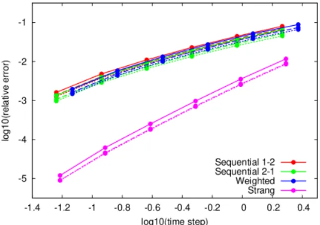
The correspondence between the “exact” and the necessary bounds will be investigated in Section 9.

It is important to compare the bounds obtained for the time step in Proposition 6.2 with the similar result obtained for a numerical method without using operator splitting, cf. bound (23).

(14)

Proposition 6.3. With Notation 5.1, we have the following assertions.

(i) The estimate −¹_bW₀ − _M^b

> _M+c¹ holds for all M, b, c > 0 with M > be.

(ii) For an arbitrary M > 0, we have the limit −¹_bW₀ − _M^b b→0

−−→ _M¹ .

Proof. (i) The relation W₀(y) < y for all y < 0, the strictly increasing of W₀, and the assumption M > be imply the assertion.

(ii) Follows from Lemma 5.2 with p=b and q=M.

Proposition 6.3 means that in the caseM > beour method (30) gives a larger upper bound for the time step τ as the application of explicit Euler method without operator splitting.

Namely, in this caseM+c > M > be> bholds, which leads tomin{1/b,1/(M+c)}= 1/(M+c).

Moreover, for the caseM ≤be, our method (30) satisfies the properties (P2)–(P4) without any restriction on the time step τ. Hence, method (30) is more convenient to use than the method proposed in [14].

We note here, that although Proposition 6.2 allows large values for the time step, the use of these is not advised, since it leads to considerable higher error in the numerical solution.

Remark 6.4. Another possible way to perform the time step analysis is to check the non- negativity preservation for each sub-problem separately, and then take the most severe constraint on the time step. In case of the sequential splitting 1–2 (30), however, we obtain a weaker result than the one presented in Proposition 6.2, namely, τ ≤ 1/M. This can be seen from the following consideration. Sub-problem (27) preserves the non-negativity for all τ >0, while sub-problem (35) introduces the constraint τ ≤ 1/M. This bound is always smaller than the one obtained in Proposition 6.2, which can be seen from the proof of Proposition 6.3/(i). Thus, the point in analysing the combined method (30) is that it might lead to sharper constrains on the time step, as it does in this case.

6.2 Sequential splitting 2–1

We study now the sequential splitting with the other order of the sub-problems. In a single time step we first solve (Sub.2) and then (Sub.1) with the appropriate initial conditions. Similarly to (24), for all n∈N and (x, y)∈Ωwe consider the iteration steps

((Sub.2) for all t ∈(nτ,(n+ 1)τ]

with initial condition X^[2](nτ, x, y) = X^spl(nτ, x, y) ((Sub.1) for all t ∈(nτ,(n+ 1)τ]

with initial condition X^[1](nτ, x, y) = X^[2]((n+ 1)τ, x, y) X^spl((n+ 1)τ, x, y) := X^[1]((n+ 1)τ, x, y)

(33)

where X^spl(0, x, y) = X₀(x, y) is the original initial value in (7) for each X ∈ {S, I, R}. Thus, we consider first the space discretised sub-problem (26) and then (25). Then the numerical

(15)

method takes the form











S_k,`^[1],n+1 =S_k,`ⁿ −τ S_k,`ⁿ T_k,`ⁿ , I_k,`^[1],n+1 =I_k,`ⁿ +τ S_k,`ⁿ T_k,`ⁿ , R^[1],n+1_k,` =Rⁿ_k,`,

(34)











S_k,`ⁿ⁺¹ = e^−cτS_k,`^[1],n+1, I_k,`ⁿ⁺¹ = e^−bτI_k,`^[1],n+1,

Rⁿ⁺¹_k,` =R^[1],n+1_k,` + (1−e^−cτ)S_k,`^[1],n+1+ (1−e^−bτ)I_k,`^[1],n+1

(35)

for all n ∈Nand (x_k, y_`)∈ G. Combination of sub-problems (34) and (35) yields the method







S_k,`ⁿ⁺¹ = e^−cτS_k,`ⁿ (1−τ T_k,`ⁿ ), I_k,`ⁿ⁺¹ = e^−bτ(I_k,`ⁿ +τ S_k,`ⁿ T_k,`ⁿ ),

Rⁿ⁺¹_k,` =Rⁿ_k,`+ (1−e^−cτ)S_k,`ⁿ (1−τ T_k,`ⁿ ) + (1−e^−bτ)(I_k,`ⁿ +τ S_k,`ⁿ T_k,`ⁿ ).

(36)

We can state the same result as before.

Proposition 6.5. Proposition 6.1 holds for the method (36).

Proof. First, we add up the equations in (36) to obtain property (P1). To prove the next assertion, we consider an arbitrary step again. Property (P2) implies that T_k,`ⁿ is non-negative.

This and e^−cτ <1 imply that S_k,`ⁿ⁺¹ ≤S_k,`ⁿ . Moreover, the non-negativity of S_k,`ⁿ⁺¹ implies that 1−τ T_k,`ⁿ ≥0, therefore, Rⁿ⁺¹_k,` ≥R_k,`ⁿ holds as well.

According to Proposition 6.5, it suffices to show the non-negativity property (P2) to obtain the monotonicity properties (P3) and (P4).

Proposition 6.6. The non-negativity property (P2) holds true for the method (36) if the time step τ satisfies the condition

τ ≤ 1

M (37)

where M is defined in Notation 5.1.

Proof. Since the initial values are non-negative, we assume thatX_k,`ⁿ ≥0and show thatX_k,`ⁿ⁺¹ ≥ 0 for all n ∈ N, (x_k, y_`) ∈ G, and X ∈ {S, I, R}. Since the assumption τ ≤ 1/M implies 1−τ T_k,`ⁿ ≥ 0, the non-negativity of S_k,`ⁿ⁺¹ is fulfilled. Furthermore, since all additive terms in the second and third equations of (36) are non-negative, we have I_k,`ⁿ⁺¹ ≥ 0 as well as R_k,`ⁿ⁺¹ ≥0.

Hence, for M +c > b we get a better bound for the time stepτ than for the explicit Euler method without splitting, cf. (23). IfM+c < b, it might happen that the bound of the non-split method is better. Since the application of operator splitting usually needs more CPU time than the explicit Euler method itself, it is not advised to use method (36) but the first one (30).

We note that in case of the sequential splitting 2–1 we obtain the same bound (37) on the time step τ both when analysing the combined method (36) or the separate sub-problems (34) and (35).

(16)

7 Weighted sequential splitting

Especially on parallel computers, it is a good idea to combine the solution to sequential splittings 1–2 and 2–1 with some Θ∈[0,1]parameter as follows:

X = Θ·X₍₃₀₎+ (1−Θ)·X₍₃₆₎

where X₍₃₀₎, X₍₃₆₎ denotes the approximate solutions obtained by numerical methods (30) and (36), respectively, for eachX ∈ {S, I, R}. We note that the choiceΘ = 0results in the method (36), while Θ = 1 gives (30). In this way we get the following numerical method:







S_k,`ⁿ⁺¹ = e^−cτS_k,`ⁿ 1−τ(Θe^−bτ + (1−Θ))T_k,`ⁿ , I_k,`ⁿ⁺¹ = e^−bτ I_k,`ⁿ +τ(Θe^−cτ + (1−Θ))S_k,`ⁿ T_k,`ⁿ

,

Rⁿ⁺¹_k,` =Rⁿ_k,`+ (1−e^−cτ)S_k,`ⁿ (1−(1−Θ)τ T_k,`ⁿ ) + (1−e^−bτ)(I_k,`ⁿ + (1−Θ)τ S_k,`ⁿ T_k,`ⁿ ).

(38)

As before, we investigate the validity of properties (P1)–(P4).

Proposition 7.1. Proposition 6.1 is valid for method (38).

Proof. The conservation of the size of the population is obtained again by adding up the equations in (38). SinceΘ,e^−bτ,e^−cτ ∈(0,1)and T_k,`ⁿ ≥0 in the first equation of (38), we have S_k,`ⁿ⁺¹ ≤ S_k,`ⁿ . Due to property (P2), all terms in the third equation of (38) are non-negative, therefore, Rⁿ⁺¹_k,` ≥Rⁿ_k,` holds true.

In order to study the non-negativity preservation (P2), we need the following notation.

Notation 7.2. For the parameterΘ∈[0,1], we define Θ^∗ := e²

e²+ 1 ≈0.8808.

It will turn out that we get remarkably different bounds for Θbeing under or above Θ^∗. Notation 7.3. (a) ForΘ∈[0,1] and b >0, we define the function V_Θ,b: R⁺→(0,+∞) as

V_Θ,b(τ) = τ(1−Θ(1−e^−bτ)).

(b) We introduce the values 0< τ₀ < τ−1 as τ−1 := ¹_b 1−W−1

e(Θ−1) Θ

for Θ∈[Θ^∗,1), τ0 := ¹_b 1−W0

e(Θ−1) Θ

for Θ∈[Θ^∗,1].

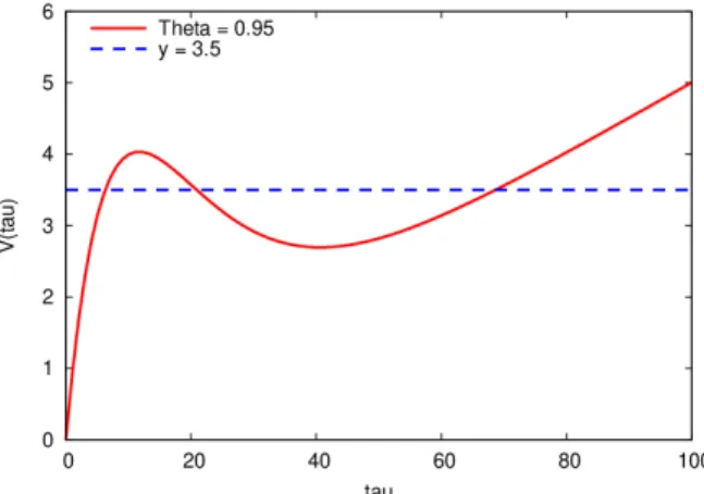
On Figure 2 the graph of function V_Θ,b is shown for Θ = 0.95 and b = 0.1. In order to illustrate its dependence on Θ, we present the graph of function V_Θ,b for various values of Θ and b = 0.1 on Figure 3.

(17)

Figure 2: Graph of function VΘ,b(τ) =τ(1−Θ(1−e^−bτ))forΘ = 0.95andb= 0.1. The horizontal line indicates the value3.5.

Figure 3: Graph of function VΘ,b(τ) =τ(1−Θ(1−e^−bτ))for Θ = 0.6, 0.8, 0.9, 0.95, 1 andb= 0.1.

7.1 Case of “small” Θ

We take now Θ∈[0,Θ^∗), and examine first whether the inverse ofV_Θ,b exists.

Lemma 7.4. For Θ ∈ [0,Θ^∗), function V_Θ,b is strictly increasing, thus, V_Θ,b⁻¹ exists, and is strictly increasing on (0,+∞).

Proof. To show that function V_Θ,b is monotone, we calculate its derivative with respect to τ:

V_Θ,b⁰ (τ) = _dτ^d τ(1−Θ(1−e^−bτ))

= (1−Θ) + Θe^−bτ(1−bτ).

We now determine its zeros:

V_Θ,b⁰ (τ) = 0 (1−Θ) + Θe^−bτ(1−bτ) = 0

e^−bτ(1−bτ) = Θ−1 Θ e^1−bτ(1−bτ) = eΘ−1

Θ .

With the notations x := 1−bτ and µ:= e(Θ−1)/Θ < 0, we need to examine the solutions x to the equation (21). The relation Θ <Θ^∗ implies µ < −1/e, hence, there is no solution x

(18)

to equation (21) according to Remark 5.3. Thus, there are no zeros of function V_Θ,b⁰ , therefore, V_Θ,b is monotone. Furthermore, V_Θ,b⁰ (1/b) = 1−Θ>0 implies that function V_Θ,b is increasing on(0,+∞). Hence, its inverse V_Θ,b⁻¹ exists and is strictly increasing on(0,+∞).

We state now the result for the non-negativity preservation.

Proposition 7.5. For Θ∈[0,Θ^∗), the non-negativity property (P2) holds for the method (38) if the time step τ satisfies the following criterion:

τ ≤V_Θ,b⁻¹ _M¹

. (39)

Proof. Since the initial values are non-negative, we treat an arbitrary step. We assumeX_k,`ⁿ ≥0 and show X_k,`ⁿ⁺¹ ≥0for all n∈N, (x_k, y_`)∈ G, and X ∈ {S, I, R}. The non-negativity of I_k,`ⁿ⁺¹ and Rⁿ⁺¹_k,` follows immediately, because all additive terms are non-negative in the second and third equations of system (38).

From the first equation in (38), S_k,`ⁿ⁺¹ is non-negative if 1−τ T_k,`ⁿ 1−Θ(1−e^−bτ)

≥0 τ 1−Θ(1−e^−bτ)

≤ 1 T_k,`ⁿ V_Θ,b(τ)≤ 1

T_k,`ⁿ .

Due to relation Θ<Θ^∗ = e²/(e² + 1) and Lemma 7.4, function V_Θ,b is strictly increasing and its inverse is well-defined on (0,+∞). Thus, we have the following bound for the time step τ:

τ ≤V_Θ,b⁻¹ _T¹n k,`

. (40)

Property (P1) implies T_k,`ⁿ ≤ M for all n ∈ N and (x_k, y_`) ∈ G. Hence, the inequality (40) is fulfilled due to Assumption (39) and since V_Θ,b⁻¹ is strictly decreasing on (0,+∞).

7.2 Case of “large” Θ

We take now Θ∈[Θ^∗,1], and examine the behaviour of function V_Θ,b. Lemma 7.6. With Notations 5.1 and 7.3, we have the following assertions.

(a) For Θ∈[Θ^∗,1), we have the following strictly monotonicity segments of function V_Θ,b: (i) on (0, τ₀) the function V_Θ,b is strictly increasing, therefore, its inverse V₁⁻¹ exists

and is strictly increasing,

(ii) on (τ₀, τ−1) the function V_Θ,b is strictly decreasing, therefore, its inverse V₂⁻¹ exists and is strictly decreasing,

(iii) on(τ−1,+∞)the functionV_Θ,b is strictly increasing, therefore, its inverseV₃⁻¹ exists and is strictly increasing

(b) For Θ = 1, the inverse of function V_1,b = τe^−bτ is strictly increasing on [0,1/b) and decreasing on (1/b,+∞).

(19)

Proof. Similarly to the proof of Lemma 7.4, we need to examine the function V_Θ,b⁰ (τ) = _dτ^d τ(1−Θ(1−e^−bτ))

= (1−Θ) + Θe^−bτ(1−bτ) for Θ∈[Θ^∗,1)and determine its zeros:

d

dτV_Θ,b(τ) = 0 e^−bτ(1−bτ) = Θ−1

Θ e^1−bτ(1−bτ) = eΘ−1

Θ .

With the notations x:= 1−bτ and µ:= e(Θ−1)/Θ<0, we need to examine the solutions x to the equation (21). SinceΘ≥Θ^∗ = e²/(e²+ 1), we have µ≥ −1/ein Remark 5.3. Thus, we have the following three cases for τ = (1−x)/b.

(i) On (0, τ₀) we examine the sign of

τ→0limV_Θ,b⁰ (τ) = lim

τ→0 (1−Θ) + Θe^−bτ(1−bτ)

= 1−Θ + Θ = 1 >0,

so functionV_Θ,b is strictly increasing, and its inverse V₁⁻¹ exists and is strictly increasing.

(ii) Since τ₁ := (1−x₁)/b= 2/b and x−1 < x₁ =−1≤x₀ implies τ₀ ≤τ₁ = ²_b < τ−1, on the interval (τ0, τ−1)we examine the sign of

V_Θ,b⁰ (²_b) = 1−e² <0,

so function V_Θ,b is strictly decreasing here, and its inverse V₂⁻¹ exists and is strictly decreasing.

(iii) On (τ−1,+∞)we examine the sign of

τ→+∞lim V_Θ,b⁰ (τ) = lim

τ→∞ (1−Θ) + Θe^−bτ(1−bτ)

= 1−Θ + lim

x→−∞xe^x= 1−Θ>0, so functionV_Θ,b is strictly increasing, and its inverse V₃⁻¹ exists and is strictly increasing.

This proves assertion (a). Since the case Θ = 1 corresponds to the sequential splitting (30), assertion (b) follows from Remark 5.3 and the considerations in the proof of Proposition 6.2.

We have then the following result for the non-negativity property in this case.

Proposition 7.7. For Θ∈[Θ^∗,1], the non-negativity property (P2) is fulfilled for the method (38) in the following cases:

(i) for _M¹ ∈(0, V_Θ,b(τ₋₁)]: if τ ≤V₁⁻¹(_M¹ ),

(ii) for _M¹ ∈(VΘ,b(τ−1), VΘ,b(τ0)]: if τ ∈ 0, V₁⁻¹(_M¹ )

or τ ∈

V₂⁻¹(_M¹), V₃⁻¹(_M¹ ) , (iii) for _M¹ > V_Θ,b(τ₀): if τ < V₃⁻¹(_M¹ )

with Notations 5.1 and 7.3.

(20)

Proof. The non-negativity of I_k,`ⁿ⁺¹ and Rⁿ⁺¹_k,` follows from the non-negativity of S_k,`ⁿ⁺¹. So we prove only the latter one. Similarly as in the proof of Proposition 7.5, we need to determine the intervals where

V_Θ,b(τ) := τ(1−Θ(1−e^−bτ))≤ 1 T_k,`ⁿ .

To do so, we need an inverse of functionV_Θ,b which has the three branches presented in Lemma 7.6. Property (P1) implies the estimate T_k,`ⁿ ≤M which provides the assertions.

Remark 7.8. As we have already pointed out, the cases Θ = 0 and Θ = 1 correspond to the sequential splitting methods (36) and (30), respectively. SinceV_1,b(τ) = τ, its inverseV_1,b⁻¹ is the identity in (39), cf. Proposition 6.6. Furthermore,V_0,b(τ) = τe^−bτ impliesV_0,b⁻¹(y) =−W(−by)/b having the two branches W = W−1 and W = W₀ as in Proposition 6.2. Hence, as expected, the corresponding results in Propositions 7.5 and 7.7 meet the conditions in Propositions 6.2 and 6.6.

Remark 7.9. As in the case of the sequential splitting 1–2 (cf. Remark 6.4), Propositions 7.5 and 7.7 yield sharper conditions of the time step than the bound is when analysing the non-negativity preservation of the sub-problems separately. This is true due to the following consideration. The weighted splitting consists of the two sequential splittings 1–2 (30) and 2–1 (36). In Proposition 6.3 we showed that the bound obtained for sequential splitting 1–2 is sharper than 1/M. Furthermore, for the sequential splitting 2–1 we have the bound 1/M. Hence, the separate treatment of the sub-problems leads to the constraint τ ≤ 1/M. The bounds obtained in the present section, however, are always sharper. In the case of “small” Θ, the bound V_Θ,b⁻¹(_M¹) is larger than 1/M, since V_Θ,b⁻¹(τ) is a strictly increasing function in τ by Lemma 7.4, and V_Θ,b⁻¹(τ) =τ holds for Θ = 0 (so the bound here is simply 1/M), furthermore, V_Θ,b⁻¹(τ)is monotonically decreasing asΘincreases. For “large” values ofΘ, we refer to Figure 3 to see that we can have three cases with respect to the location of the graph of functionV_Θ,b(τ) relative to the horizontal line1/M. In all cases we have∂V_Θ,b(τ)/∂Θ<0, that is, the left point of intersection moves to the right when the value of Θ is increasing (the movement might not be continuous but monotone). This means that the left bound is increasing as well.

8 Strang splitting

In contrast to the sequential splittings presented in Sections 6.1 and 6.2, Strang splitting needs three steps with the two sub-problems (Sub.1)–(Sub.2): the first step uses (Sub.1) with time step τ /2, the second uses (Sub.2) with time step τ, and the third uses (Sub.1) again with time step τ /2, always using the previous solution as an initial condition. Moreover, while the sequential splitting is of first order, the Strang is a second-order method. Therefore, by [2], we need to use a second-order time discretisation method to avoid order reduction. Hence, sub-problem (Sub.2) will be solved by Heun’s method as presented in (15)–(16).

We note that the choice of (Sub.2) being the middle step is explained by the fact that it needs more computational effort and time than sub-problem (Sub.1). Hence, computing it only once at each step is more efficient than using the approach having (Sub.1) in the middle, since in that case (Sub.2) should be evaluated twice.