Runway Relative Positioning of Aircraft with IMU-Camera Data Fusion ?

(1)

Runway Relative Positioning of Aircraft with IMU-Camera Data Fusion ?

Tamas Grof^∗ Peter Bauer^∗ Antal Hiba^∗∗Attila Gati^∗∗

Akos Zarandy^∗∗ Balint Vanek^∗

∗Systems and Control Laboratory, Institute for Computer Science and Control, Hungarian Academy of Sciences, Budapest, Hungary (e-mail:

bauer.peter@sztaki.mta.hu).

∗∗Computational Optical Sensing and Processing Laboratory, Institute for Computer Science and Control, Hungarian Academy of Sciences,

Budapest, Hungary (e-mail: hiba.antal@sztaki.mta.hu)

Abstract: In this article the challenge of providing precise runway relative position and orientation reference to a landing aircraft based-on monocular camera and inertial sensor data is targeted in frame of the VISION EU H2020 research project. The sensors provide image positions of the corners of the runway and the so-called vanishing point and measured angular rate and acceleration of the aircraft. Measured data is fused with an Extended Kalman Filter considering measurement noise and possible biases. The developed method was tested with computer simulated data considering Matlab/Simulink simulation of the aircraft and the processing of artificial images from Flightgear. This way the image generated noise and the uncertainties in image processing are considered realistically. Inertial sensor noises and biases are generated in the Matlab simulation. A large set of simulation cases was tested guiding the landing aircraft based-on ILS. The results are promising so completing ILS or SBAS information with the estimates can be a next step of development.

Keywords:Aircraft operation, Computer vision, Vision-inertial data fusion 1. INTRODUCTION

In recent years several projects aimed to provide analytical redundancy and additional information sources to onboard aircraft systems. As camera sensors become more and more popular not only on unmanned aerial vehicles (UAVs) but also on passenger airplanes (Gibert et al. (2018)) they can be considered as an additional source of information. A research project targeting to explore the possibilities to use camera systems as additional information sources during aircraft landing is a Europe-Japan collaborative project called VISION (Validation of Integrated Safety-enhanced Intelligent flight cONtrol) (see VISION (2016)). VISION focuses on critical flight scenarios especially on near-earth maneuvers and aims to improve the overall precision level of the navigational systems currently used by aircraft. To meet these expectations methods with combined GPS- ILS-Camera data are being developed and tested with the goal to preserve the acceptable level of safety even if one

? This is the author version of article published at IFAC ACA 2019 Conference (IFAC).c This paper was supported by the J´anos Bolyai Research Scholarship of the Hungarian Academy of Sciences. The research presented in this paper was funded by the Higher Education Institutional Excellence Program. The research leading to these results has received funding from the European Union’s Horizon 2020 research and innovation programme under grant agreement No. 690811 and the Japan New Energy and Indus- trial Technology Development Organization under grant agreement No. 062600 as a part of the EU/Japan joint research project entitled

’Validation of Integrated Safety-enhanced Intelligent flight cONtrol (VISION)’.

of the three sensory systems has degraded performance see Watanabe et al. (2019). In this article an additional method is presented which can augment the GPS-ILS- Camera fusion by integrating inertial measurement unit (IMU) and camera data. Vision integrated navigation is an extensively researched topic so only few relevant references are cited. Strydom et al. (2014) applies stereo vision and optic flow to position a quadcopter along a trajectory.

The introduced method requires several hundred (400 in the example) points to be tracked, considers estimated orientation from an IMU and is limited to 0-15m altitude range because of the stereo vision. The method introduced in Conte and Doherty (2009) considers monocular vision with geo-referenced aerial images database. Visual odometry with Kalman filter and acceleration bias state is used and at least 4 identified points in the image are required.

Ground relative position, velocity and orientation are estimated without gyroscope bias and there can be an observability issue of the heading in hovering mode. Real flight test results are presented applying three onboard comput- ers on the Yamaha Rmax helicopter. Weiss et al. (2013) introduces a method which uses IMU-Camera fusion in GPS denied environment to estimate aircraft position, velocity and orientation in a loosely coupled system. It develops the image processing part to provide 6D position information and couples it with an Error State Kalman Fil- ter (ESKF) which considers image scale and possible drifts of the vision system. It also estimates acceleration and angular rate sensor biases. Nonlinear observability analysis is performed and real flight test results underline the ap-

(2)

plicability of the method. Gibert et al. (2018) considers the fusion of monocular camera with IMU to determine runway relative position assuming that IMU provides ground relative velocity and orientation with sufficient precision and the runway sizes are unknown. Finally, Watanabe et al. (2019) considers position and orientation estimation relative to a runway with known sizes during landing (in frame of the VISION project) and applies an ESKF for GNSS-Camera loose/tight data fusion considering the delay in image processing. The estimated parameters are relative position, velocity, orientation and sensor biases.

The results of extensive simulation are presented together with the steps toward real flight validation. In Martinelli (2011) a closed-form solution was proposed for orientation and speed determination by fusing monocular vision and inertial measurements. In the article an algorithm is presented where the position of the features and the vehicle speed in the local frame and also the absolute roll and pitch angles can be calculated. In order to calculate these values the camera needs to observe a feature four times during a very short time interval. The strengh of this method is that it is capable to calculate the said states of the aircraft without any initialization and perform the estimation in a very short time, but the observability analysis which was done in the paper showed that the aicraft’s absolute yaw angle can’t be estimated using this particular method.

Huang et al. (2017) focuses on estimating the absolute position, velocity and orientation values for a UAV. That article proposes an absolute navigation system based on landmarks which positions are known in advance. With the help of these landmarks the paper considers a navigation filter design by fusing a monocular camera and IMU without considering the possible measurement biases of the latter. They restrict the number of landmarks to three and execute observability analysis. After this an Extended and an Unscented Kalman Filter (UKF) design are proposed to address the problem. Between these two filter designs a comparison is presented in regards of precision levels which showed that the UKF is superior.

The method that is presented in this paper focuses on calculating an aircraft’s runway relative position, velocity and orientation applying the fusion of IMU measurements and monocular images. Possibly stereo images can be more effective but resonances can cause more problems (synchronization of the images) and stereo vision has range limitation also (Strydom et al. (2014)). Our method considers only 3 reference points related to the runway:

the corners and the vanishing point in the direction of the runway. This is much less than the several tens or hundreds points in Strydom et al. (2014) and Weiss et al.

(2013) and does not require geo-referenced images as Conte and Doherty (2009). The only required information to be known is the width of the runway as in Watanabe et al. (2019) there is no need for absolute position of any point. Though the method published in Gibert et al.

(2018) does not require any information about the runway they assume that the IMU provides precise velocity and orientation information which is not true for a UAV with low grade IMU. Compared to Martinelli (2011) our method targets to estimate also the yaw angle (by considering the vanishig point). Compared to Huang et al. (2017) we also target to estimate the angular rate and acceleration biases and consider EKF because we assume that the filter can

be initialized with close to the real data from GPS and/or ILS.

The structure of the article is as follows. Section 2 summarizes the system equations and examines the observability of the system, Section 3 introduces the simulation setup while Section 4 summarizes the performance of the algorithm based-on simulation data. Finally Section 5 con- cludes the paper.

2. SYSTEM EQUATIONS

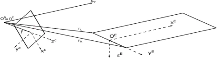
Firstly, we have to define the coordinate systems. These are the fixed runway inertial frame (XÊ, YÊ, ZÊ) which centerpoint (OÊ) was defined as the center of the runway’s threshold line, the body frame (X^B, Y^B, Z^B) which is rotated and translated compared to the inertial frame, and lastly the camera frame (X^C, Y^C, Z^C) which is assumed to have a shared centerpoint with the body frame but its axes are swapped according to Fig. 1.

x^E

y^E z^E

b b

x^c z^c y^c

f O^E

rR rL O^B=O^C

rvp

Fig. 1. Coordinate systems

In this paper the mathematical model is formulated by the aircraft kinematic equations including the following variables:

x=

v^T_B p^T q^T^T

(1) u=

a^T_B ω_B^T^T

(2) b=

b^T_a b^T_ω^T

(3) η =

η^T_a η_ω^T η^T_ba η^T_bω^T

(4) ν =

ν_z^T_L ν_z^T_R ν_z^T_vp^T

(5) y=

z_L^T z_R^T z_vp^T ^T

(6) Where x is the state vector with vB runway relative velocity in the body systemprunway relative position and q the quaternion representation of orientation. u is the input including the measurements gathered by the IMU sensor with a_B being the measured acceleration and ω_B the angular rate vector in body frame, while b contains the bias parameters influencing the accelerometers and gyroscopes. The η vector consists of the process noise variables that are affecting the IMU measurements and the IMU bias values. This case ηa and ηω refer to the noise that affect the inertial measurements, while ηba and ηbω

influence the bias values (modeled as first order Markov processes). The measurement noise parameters for the pixel coordinates of the reference points are in theνvector, where νz_L, νz_R, νz_vp are the measurement noise values that distort the measured pixel coordinates of the left, right corner and the vanishing point respectively. Finally, yincludes the camera measurement data, wherezL,zR, are the image plane coordinates of the left and right corners

(3)

of the runway and z_vp is the projection of the vanishing point (see (14) to (16)).

The kinematic equations that describe the aircraft motion can be written as follows

˙

v_B=V_Bω_B−V_B(b_ω+η_ω) +a_B−b_a+e^G_Bg−η_a (7)

˙

p=T_EBv_B (8)

˙

q=−Q(q)ωB+Q(q)(bω+ηω) (9)

b˙= [I2 0]η (10)

Where V_B is the matrix representation of the v_B× cross product operator,TEB is the body to runway transforma- tion matrix andQ(q) is the matrix with quaternion terms in the quaternion dynamics similarly as in Weiss et al.

(2013).e^G_Bgis the gravitational acceleration in body frame andI2 is the two dimensional unit matrix and 0 is a zero matrix with appropriate dimension.

The output equations were formulated by using a per- spective camera projection model. The first two reference points are the corners of the runway while the third reference point is the so called vanishing point aligned with the runway’s heading direction (it coincides with the runway system x axis). The camera frame coordinates of these points can be obtained as:

rL=TCBTBE(fL−p) (11) r_R=T_CBT_BE(f_R−p) (12) r_vp=T_CBT_BE

"1 0 0

#

(13) Where TCB is the rotation matrix from body to camera frame. f_L and f_R are the left and right coordinates of threshold’s corners in the runway’s frame while [1 0 0]^T is the direction of the vanishing point in the runway frame.

Finally, the relation between the image plane and the camera frame coordinates can be defined as follows considering subscriptsx, y, zas the coordinates of the vectors and the measurement noises also:

z_L= f r_L,z

rL,x

rL,y

+ν_z_L (14)

z_R= f rR,z

rR,x

r_R,y

+ν_z_R (15)

zvp= f rvp,z

rvp,x

r_vp,y

+νz_vp (16)

2.1 Observability

Considering the whole system of equations (7) to (10) its a nonlinear system (17) in input affine form so observability

should be checked accordingly based-on Vidyasagar (1993) for example.

˙

x=f(x, η) +

m

X

i=1

gi(x)ui

y=h(x, ν)

(17)

Local observability of such a system can be checked by calculating the observability co-distribution (for details see Vidyasagar (1993)). This calculation can be done by applying the Matlab Symbolic Toolbox. Checking the rank of the symbolic result usually gives full rank as symbolic variables are considered by the toolbox as nonzero. On the contrary there can be several zero parameters in the co-distribution in a special case that’s why special configurations with zero parameters should be carefully checked.

For our system the acceleration (a), angular rate (ω) and their biases (ba, bω) can be zero in special cases and the orientation (q) can be parallel with the runway (considered as ’zero quaternion’). The runway relative position and velocity can not be zero if we are on approach. The nonzero orientation is considered to be aligned with a given nonzero glide slope γ. The rank of the co-distribution was tested for several combinations of zero and nonzero parameters and it resulted to be full rank in all cases. So the system should be locally observable in every possible case. The examined combinations of special cases are summarized in Fig. 2. The horizontal axis shows the possibly zero parameters, the vertical axis shows the examined 17 cases (one case / row) where×-s show the zero value of a parameter in the given case. Though the examined cases do not cover all the possibilities we think that it covers enough cases to detect any uncertainty in observability.

Fig. 2. Examined special combinations in observability check

3. MATLAB AND FLIGHTGEAR SIMULATION The implemented EKF algorithm was tuned and tested in a Matlab/Simulink environment. This consists of the Matlab simulation of K-50 aircraft synchronized with the Flightgear based generation and processing of runway image giving finally zL, zR, zvp. The camera modeled in

(4)

FlightGear has a resolution of 1280 ×960 pixels with 30^◦ horizontal field of view. The real data, which will be compared to the filter’s results to get an estimate of the filter’s precision includes aircraft runway relative position, velocity and orientation and was generated inside the K-50 aircraft simulation. The considered acceleration and angular rate measurments are also generated by the simulation including biases and noises also. The simulation uses an ILS (Instrumental Landing System) model to guide the aircraft towards the runway. It is important to note that the IMU and the image processing work with different measurement frequency, so when implementing the EKF algorithm the correction step is only applied when the camera has observed the required pixel coordinates other- wise only the prediction steps are propagated. During the simulation the IMU unit’s frequency was 100Hzwhile the camera’s frequency was set to 10Hzas in the real hardware system. The delays of image processing (see Watanabe et al. (2019)) are neglected here as the simulation can run slower than real time.

After the implementation and tuning (through the covariance matrices by trial and error) of the EKF several test scenarios were defined in order to check if the algorithm works in different cases. The considered initial positions are summarized in Table 1.

Table 1. Simulated initial positions

Case Description

1 Aircraft starts on the glide slope 2 Vertical or horizontal offset from the glide slope 3 Both vertical and horizontal offset

Furthermore, for every initial position the following sensor configurations were considered:

Table 2. Simulated sensor setups

Setup Description

1 Simulation without any bias or noise 2 Simulation with process and measurement noise, but

no inertial sensor bias

3 Simulation with either acceleration or angular rate bias, but without noise

4 Simulation with all of the inertial sensor biases and process and measurement noises

Fig. 3. FlightGear with image processing from Hiba et al.

(2018)

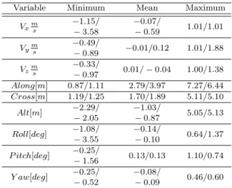
Table 3. Minimum, Maximum and Mean values of the simulations 1/1 and 3/4

Variable Minimum Mean Maximum

Vxm s

−1.15/

−3.58

−0.07/

−0.59 1.01/1.01 Vym

s

−0.49/

−0.89 −0.01/0.12 1.01/1.88 Vzm

s

−0.33/

−0.97 0.01/−0.04 1.00/1.38 Along[m] 0.87/1.11 2.79/3.97 7.27/6.44 Cross[m] 1.19/1.25 1.70/1.89 5.11/5.10

Alt[m] −2.29/

−2.05

−1.03/

−0.87 5.05/5.13 Roll[deg] −1.08/

−3.55

−0.14/

−0.10 0.64/1.37 P itch[deg] −0.25/

−1.56 0.13/0.13 1.10/0.74 Y aw[deg] −0.25/

−0.52

−0.08/

−0.09 0.46/0.60

4. RESULTS

All possible scenarios described in Section 3 Tables 1 and 2 were run in Matlab. All of the simulations were initialized with estimation errors which were set as 5m for position, 1^m_s for velocity and 1^◦for Euler angles (see the figures). In this chapter two scenarios – the best and the worst – are presented in detail as the estimation results of the other scenarios are very similar. The given figures (Fig. 4 to 9) show the estimation errors with dashed lines, while the approximated steady state errors as continuous lines.

In the first case the aircraft starts the landing from a position located on the glide slope and there are no additional noises or sensor biases added to the system (simulated case 1/1). This is considered as a best case scenario (every- thing known perfectly) and the errors relative to the real (simulated in Matlab) values remain small as expected.

Figures 4 and 6 show that the difference between the real values and the aircraft’s estimated velocity and orientation converges around zero, while Fig. 5 presents the runway relative position errors of the vehicle converging to nonzero values. The K-50 Simulink simulation uses runway relative values in meters, while the Flightgear is fed by the Latitude-Longitude-Altitude (LLA) coordinates. The conversion between relative terms to global values causes that the simulated camera measurements aren’t perfect, which can results in errors in the position estimation.

The second case (simulated case 3/4) includes the results for the worst scenario with initial horizontal and vertical offsets and all sensor biases and noises. The results of this case (Fig. 7 to 9) show larger deviations from the real values before the convergence occurs but these are also acceptable. The noise causes the estimation errors to continuously alternate around the steady state values with an acceptable amplitude.

The rate of convergence is a bit smaller in the worst case then in the best. It is greatly affected by the filter’s covariance matrices, which were set the same for all the simulations. Possibly by further tuning the covariances better convergence can be obtained. The introduction of the sensor biases increased the transient errors but then the steady state error levels are similar. After running all

(5)

5 10 15 20 25 30 Time [s]

-4 -2 0 2

Vx error [m/s]

5 10 15 20 25 30

Time [s]

-1 0 1 2

Vy error [m/s]

5 10 15 20 25 30

Time [s]

-1 0 1 2

Vz error [m/s]

Fig. 4. Estimated velocity deviation from real data in simulated case 1/1

5 10 15 20 25 30

Time [s]

0 3 5

Along error [m]

5 10 15 20 25 30

Time [s]

01 5

Cross error [m]

5 10 15 20 25 30

Time [s]

-2 0 2 4 6

Altitude error [m]

Fig. 5. Estimated position deviation from real data in simulated case 1/1

5 10 15 20 25 30

Time [s]

-4 -2 0 2

Roll error [deg]

5 10 15 20 25 30

Time [s]

-2 0 2

Pitch error [deg]

5 10 15 20 25 30

Time [s]

-1 0 1

Yaw error [deg]

Fig. 6. Estimated orientation deviation from real data in simulated case 1/1

5 10 15 20 25 30 35

Time [s]

-4 -2 0 2

Vx error [m/s]

5 10 15 20 25 30 35

Time [s]

-1 0 1 2

Vy error [m/s]

5 10 15 20 25 30 35

Time [s]

-1 0 1 2

Vz error [m/s]

Fig. 7. Estimated velocity deviation from real data in simulated case 3/4

5 10 15 20 25 30 35

Time [s]

0 3 5

Along error [m]

5 10 15 20 25 30 35

Time [s]

01 5

Cross error [m]

5 10 15 20 25 30 35

Time [s]

-2 0 2 4 6

Altitude error [m]

Fig. 8. Estimated postition deviation from real data in simulated case 3/4

5 10 15 20 25 30 35

Time [s]

-4 -2 0 2

Roll error [deg]

5 10 15 20 25 30 35

Time [s]

-2 0 2

Pitch error [deg]

5 10 15 20 25 30 35

Time [s]

-1 0 1

Yaw error [deg]

Fig. 9. Estimated orientation deviation from real data in simulated case 3/4

(6)

5 10 15 20 25 30 35 Time [s]

-1 -0.5 0 1

bax [m/s2]

Estimated bias Real bias

5 10 15 20 25 30 35

Time [s]

0 0.4 1

bay [m/s2]

5 10 15 20 25 30 35

Time [s]

0 0.81 baz [m/s2]

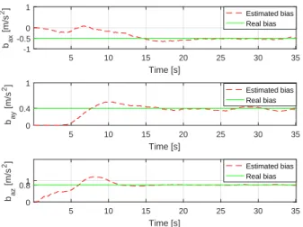
Fig. 10. Estimated accelometer bias in simulated case 3/4 the simulation cases (from 1/1 to 3/4) it can be concluded that bias parameters have a bigger relevance in the early stages of the estimation as they cause greater transient errors while the noises cause some random differences later after the convergence. The results show that the velocity and orientation of the aircraft can be estimated with close to zero errors after 10-15s convergence. The steady state error of the along and cross positions can be as large as 3-5m and 1m respectively but these are acceptable even in precision landing. However, the−2m altitude error could pose problems during the landing as it estimates UAV position 2m higher than the rel value. If this error comes from the position conversion error between simulation and Flightgear than it is acceptable if not then it should be considered in the overall system.

Furthermore, not only the position, velocity and orientation values can be estimated using the proposed method but also the bias values that are affecting the accelerometers and gyroscopes as it can be seen in Fig. 10. During the simulations the sensor bias values were set as [−0.5 0.4 0.8]^T[^m_s2] for the accelometer and [−0.3 −0.2 0.1]^T[^rad_s ] for the gyroscope and estimated well by the EKF in all cases.

5. CONCLUSION

In this paper an estimation method is presented for fusing inertial and camera sensors to help aircraft navigation during the landing phase. It applies an Extended Kalman Filter. The proposed algorithm is capable to estimate aircraft position, velocity and orientation relative to the runway and the biases of the acceleration and angular rate sensors requiring only the knowledge of the runway width.

After showing that the formulated mathematical model is locally state observable, the implemented method was tested for different landing scenarios in Matlab/Simulink and Flightgear to ensure the filter operates under different circumstances. Flightgear implements artificial runway image generation and processing to consider realistic uncertainties of this process. The filter showed promising results in regards of estimating the desired states and sensor biases with acceptable precision levels and also

with reasonable estimation convergence times. The only questionable result is the -2m offset in the estimated altitude which could result from the uncertainty of conversion between Matlab simulation (relative position in meters) and Flightgear (LLA coordinates). This should be checked before further applying the method. Future work will include reformulation as Error State Kalman Filter and consideration of image processing delays similar to Watanabe et al. (2019), application considering real flight test data and finally the fusion with ILS and/or SBAS systems at least in simulation.

REFERENCES

Conte, G. and Doherty, P. (2009). Vision- Based Unmanned Aerial Vehicle Navigation Using Geo-Referenced Information. EURASIP Journal on Advances in Signal Processing, 2009(1), 387308. doi:10.1155/2009/387308. URL https://doi.org/10.1155/2009/387308.

Gibert, V., Plestan, F., Burlion, L., Boada-Bauxell, J., and Chriette, A. (2018). Visual estimation of deviations for the civil aircraft landing. Con- trol Engineering Practice, 75, 17 – 25. doi:

https://doi.org/10.1016/j.conengprac.2018.03.004.

Hiba, A., Szabo, A., Zsedrovits, T., Bauer, P., and Zarandy, A. (2018). Navigation data extraction from monocular camera images during final approach. In 2018 International Conference on Un- manned Aircraft Systems (ICUAS), 340–345. doi:

10.1109/ICUAS.2018.8453457.

Huang, L., Song, J., and Zhang, C. (2017). Ob- servability analysis and filter design for a vision inertial absolute navigation system for UAV using landmarks. Optik, 149, 455 – 468. doi:

https://doi.org/10.1016/j.ijleo.2017.09.060.

Martinelli, A. (2011). Closed-Form Solutions for Attitude, Speed, Absolute Scale and Bias Deter- mination by Fusing Vision and Inertial Measure- ments. Research Report RR-7530, INRIA. URL https://hal.inria.fr/inria-00569083.

Strydom, R., Thurrowgood, S., and Srinivasan, M.V.

(2014). Visual Odometry : Autonomous UAV Naviga- tion using Optic Flow and Stereo.

Vidyasagar, M. (1993).Nonlinear Systems Analysis. Pren- tice Hall.

VISION (2016). Vision project webpage. URL https://w3.onera.fr/h2020 vision/node/1.

Watanabe, Y., Manecy, A., Hiba, A., Nagai, S., and Aoki, S. (2019). Vision-integrated navigation system for aircraft final approach in case of gnss/sbas or ils failures. AIAA SciTech Forum. American Institute of Aeronautics and Astronautics. doi:10.2514/6.2019-0113.

URLhttps://doi.org/10.2514/6.2019-0113.

Weiss, S., Achtelik, M., Lynen, S., Achtelik, M., Kneip, L., Chli, M., and Siegwart, R. (2013). Monocular vision for long-term micro aerial vehicle state estimation: A compendium. J. Field Robotics, 30, 803–831.