Absolute Pose Estimation of Central Cameras Using Planar Regions

(1)

Absolute Pose Estimation of Central Cameras Using Planar Regions

Robert Frohlich, Levente Tamas Member, IEEE , and Zoltan Kato Senior Member, IEEE

Abstract—A novel method is proposed for the absolute pose estimation of a central 2D camera with respect to 3D depth data without the use of any dedicated calibration pattern or explicit point correspondences. The proposed method has no specific assumption about the data source: plain depth information is expected from the 3D sensing device and a central camera is used to capture the 2D images. Both the perspective and omnidirectional central cameras are handled within a single generic camera model. Pose estimation is formulated as a 2D-3D nonlinear shape registration task which is solved without point correspondences or complex similarity metrics. It relies on a set of corresponding planar regions, and the pose parameters are obtained by solving an overdetermined system of nonlinear equations. The efficiency and robustness of the proposed method were confirmed on both large scale synthetic data and on real data acquired from various types of sensors.

Index Terms—Pose estimation, calibration, data fusion, registration, Lidar, omnidirectional camera

✦

1 I

NTRODUCTION

A

^BSOLUTEpose estimation consists of determining the position and orientation of a camera with respect to a 3D world coordinate frame. It is a fundamental building block in various computer vision applications, such as robotics (e.g. visual odometry [1], localization and navigation [2]), augmented reality [3], geodesy, or cultural heritage [4]. The problem has been extensively studied yielding various formulations and solutions. Most of the approaches focus on a single perspective camera pose estimation using n 2D–3D point correspondences, known as the Perspective n Point (PnP) problem [5], [6], [7]. It has been widely studied for large n as well as for the minimal case of n = 3 (see [7] for a recent overview).

Using line correspondences yields the Perspective n Line (PnL) problem [8], [9] (see [8] for a detailed overview).

Several applications dealing with multimodal sensors make use of fused 2D radiometric and 3D depth information from uncalibrated cameras. The availability of 3D data has also became widespread. Classical image-based techniques, such as Structure from Motion (SfM) [10] provide 3D measurements of a scene, while modern range sensors (e.g. Lidar, ToF) record 3D structure directly. Therefore methods to estimate absolute pose of a camera based on 2D measurements of the 3D scene received more attention [7],

• R. Frohlich and Z. Kato are with the Department of Image Processing and Computer Graphics, University of Szeged, P.O. Box 652, H-6701 Szeged, Hungary. Fax:+36 62 546 397, Tel:+36 62 546 399.

E-mail:{frohlich,kato@inf.u-szeged.hu}

• Z. Kato is with the Department of Mathematics and Informatics, J.

Selye University, Komarno, Slovakia.

• L. Tamas (Corresponding author) is with the Automation Department from the Technical University of Cluj-Napoca, Memorandumului st 28, 400114 RO, Tel/fax: +40 264 401 586; and with the Department of Electrical Engineering and Information Systems, University of Pan- nonia, Veszprem, HU.

E-mail: Levente.Tamas@aut.utcluj.ro

[11], [12]. Many of these methods apply to general central cameras (both perspective and omnidirectional) that are often represented by a unit sphere [13], [14], [15], [16].

Pose estimation (also known as external calibration) of 2D color and 3D depth cameras was performed especially for environment mapping applications [17]. While internal calibration can be solved in a controlled environment, e.g.

using special calibration patterns, pose estimation must rely on the actual images taken in a real environment. Popular methods rely on point correspondences such as [18], or using fiducial markers [19], which may be cumbersome to use in real life situations. This is especially true in a multimodal setting, where omnidirectional images need to be combined with other non-conventional sensors like Lidar scans providing range only data. The Lidar-omnidirectional camera calibration problem was analyzed from different perspectives. In [20], the calibration is performed in natural scenes, however point correspondences between the 2D-3D images are selected in a semi-supervised manner. In [21], calibration is tackled as an observability problem using a (planar) fiducial marker as calibration pattern. In [22]

a fully automatic method is proposed based on mutual information (MI) between the intensity information from the depth sensor and the omnidirectional camera, while in [23], [24] a deep learning approach for calibration is presented. Another global optimization method uses the gradient orientation measure as described in [17]. However, these methods require range data with recorded intensity values, which are not always available. In real life applications, it is also often desirable to have a flexible one step calibration for systems which do not necessarily contain sensors fixed to a common platform.

In this work we propose a straightforward absolute pose estimation method which overcomes the majority of these limitations, i.e. by not using any artificial marker or intensity information from the depth data. Instead, our

(2)

0162-8828 (c) 2019 IEEE. Personal use is permitted, but republication/redistribution requires IEEE permission. See http://www.ieee.org/publications_standards/publications/rights/index.html for more method makes use of a segmented planar region from the

2D and 3D visual data and handles the absolute pose estimation problem as a nonlinear registration task. More specifically, inspired by the 2D registration framework presented in [25], for the central camera model we construct an overdetermined set of equations containing the unknown camera pose. By solving this system of equation we obtain the required set of parameters representing the camera pose.

1.1 Related work

Due to the large number of applications using central camera systems, also the range of the calibration methods is rather wide. Beside solving the generic 2D-3D registration problem, several derived applications exists including med- ical [26], robotics [17] and cultural heritage ones [4]. For the pose estimation in known environment a good example can be found in [27], while in [28] an application is reported using spherical image fusion with spatial data. A more generic classification of the types of algorithms is presented in [29]. Beside the direct measured relative pose methods such as [30], a number of generic methods are summarized below.

Several feature based methods based on specific markers are used for extrinsic camera calibration [31], [32]. In the early work of [33], alignment based on a minimal number of point correspondences is proposed, while in [34], a large number of 2D-3D correspondences are used with possibly redundant or mismatched pairs. [35] was among the first addressing the extrinsic calibration of 3D Lidar and low resolution perspective color camera, which generalized the algorithm proposed in [36]. This method is based on manual point feature selection from both domains and assumes a valid camera intrinsic calibration. A similar manual point feature correspondence based approach is proposed in [20].

Recently, increasing interest is manifested in various calibration setups ranging from high-resolution spatial data [37]

to low-resolution commercial cameras [38], as well as online calibration of depth and color sensors on a moving platform [22], [39].

A popular alternative to feature based matching is the color-intensity mutual information (MI) alignment between the 2D color image and the 3D data with intensity information such [40], [17]. Extensions to the simultaneous intrinsic-extrinsic calibration are presented in [21], which makes use of Lidar intensity information to find correspondences between the 2D-3D data. Other works are based on the fusion of IMU or GPS information for calibration [41].

A good overview of statistical methods based calibration methods can be found in [26]. Mutual information and particle filters are used in [17], which performs pose estimation using the whole image space of a single 2D-3D observation. The method can use both intensity and normal distribution information for the 3D data. A further extension of this approach based on gradient orientation measure is described in [42]. A gradient information extraction and global matching between the 2D color and 3D reflectivity information is presented in [22]. This has two major differ- ences compared to our work. Our approach is not limited

to Lidar systems with reflectivity information rather it is based only on depth information. On the optimization side, the proposed method is not restricted to convex problems and allows camera calibration using only a single Lidar- camera image pair.

An early and efficient silhouette based registration method is presented in [43], which solves a model-based vision problem using parametric description of the model.

This method can be used with an arbitrary number of parameters describing the object model and is based on global optimization with the Levenberg-Marquardt method.

A whole object silhouette based registration is proposed in [40], where the authors describe the 2D-3D registration pipeline including segmentation, pixel level similarity measure and global optimization. Although the proposed method can be used in an automatic manner, this is limited only to scenes with highly separable foreground- background parts. By an automatic segmentation of the relevant forms in panoramic images, which are registered against cadastral 3D models the segmented regions are aligned using particle swarm optimization in [44]. An extension of silhouette based registration is proposed in [45], where a hybrid silhouette and key-point driven approach is used for the registration of the 2D and 3D data. The advantage of this method is the possibility of multiple image registration as well as precise output of the algorithm.

1.2 Contributions

Instead of establishing 2D-3D point matches, relying on artificial markers or recorded intensity values, we propose a pose estimation algorithm which works on corresponding segmented 2D-3D regions. Since segmentation is anyway required in many real-life image analysis tasks, such regions may be available or straightforward to detect. Inspired by [25], we reformulate pose estimation as a shape alignment problem. The solution is obtained by constructing a system of non-linear equations, which is solved in the least squares sense by a standard Levenberg-Marquardt algo- rithm. The result represents the estimates for the unknown pose parameters. We formulate the problem as the pose estimation of an universal central camera, which includes omnidirectional as well as perspective cameras. Our method was quantitatively evaluated on a large synthetic dataset and proved to be robust and efficient on real data too. For the real tests we used both publicly available dataset, as well as our own captured data.

2 R

^EGION

-

^BASED

P

^OSE

E

^STIMATION

Pose estimation consists in computing the position and orientation of a camera with respect to a 3D world coordinate system W. Herein, we are interested in central cameras, where the projection rays intersect in a single point called projection center or single effective viewpoint.

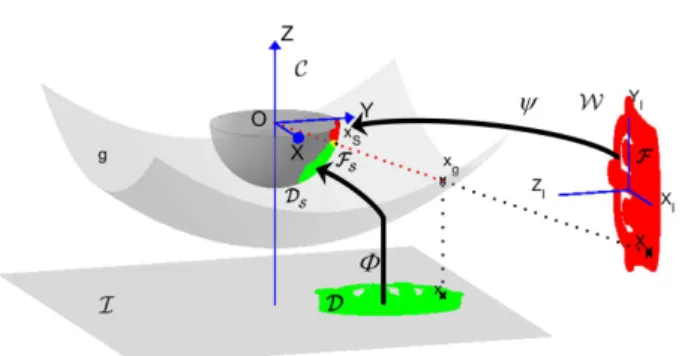
Typical examples include omnidirectional cameras as well as traditional perspective cameras. A broadly used unified model for central cameras represents a camera as a projection onto the surface of a unit sphereS (see Fig. 1) [13],

(3)

0162-8828 (c) 2019 IEEE. Personal use is permitted, but republication/redistribution requires IEEE permission. See http://www.ieee.org/publications_standards/publications/rights/index.html for more [14], [15], [16], the projection center being the center of

the sphere. The camera coordinate system C is in S, the origin is the effective viewpoint (which is also the center of the sphere) and theZ axis is the optical axis of the camera which intersects the image plane in the principal point. The absolute pose of our central camera is defined as the rigid transformation (R,t) :W → C acting between the world coordinate frame W and the camera coordinate frame C, while the internal projection function of the camera defines how 3D points are mapped from C onto the image plane I.

Let us first see the relationship between a point x = [x1, x2]^⊤ ∈ R² in the image I and its representation x_S = [xS,1, xS,2, xS,3]^⊤ ∈ R³ on the unit sphere S (see Fig. 1). Note that only the half sphere on the image plane side is actually used, as the other half is not visible from image points. There are several well known geometric models for the internal projection [13], [14], [15], [16].

Following [16], the nonlinear (but symmetric) distortion of central omnidirectional cameras is represented by a surface g between the image plane and the unit sphere S, which is rotationally symmetric around Z. Herein, as suggested by [16], we will use a fourth order polynomial

g(kxk) =a0+a2kxk²+a3kxk³+a4kxk⁴, (1) which has4parameters(a0, a2, a3, a4)representing the internal parameters of the camera. Note that for a perspective camera g is a plane – this special case will be discussed later in Section 2.2. The bijective mapping Φ :I → S is composed of

1) lifting the image pointx∈ I onto the g surface by an orthographic projection

x_g=

x

a0+a2kxk²+a3kxk³+a4kxk⁴

(2) 2) then centrally projecting the lifted pointx_g onto the

surface of the unit sphereS: x_S = Φ(x) = x_g

kx_gk (3) Thus the camera projection is fully described by means of unit vectors x_S in the half space ofR³.

The projection of a 3D world point X = [X1, X2, X3]^⊤ ∈ R³ in the generalized spherical camera is basically a central projection ontoS taking into account the extrinsic pose parameters (R, t). Thus for a world point X and its image x ∈ I, the following holds on the surface of S:

Φ(x) =x_S = Ψ(X) = RX+t

kRX+tk (4) A classical solution of the absolute pose problem is to establish a set of 2D-3D point matches using e.g. a special calibration target [38], [21], or feature-based correspondences and then solve for (R,t) via the minimization of some error function based on (4). However, in many practical applications, it is not possible to use a calibration target and most 3D data (e.g. point clouds recorded by a

Fig. 1: Spherical camera model

Lidar device) will only record depth information, which challenges feature-based point matching algorithms.

Therefore the question naturally arises: what can be done when neither a special target nor point correspondences are available? Herein, we present a solution for such challenging situations. In particular, we will show that by identifying a single planar region both in 3D and the camera image, the absolute pose can be calculated. Of course, this is just the necessary minimal configuration. More such regions are available, a more stable pose is obtained. Our solution is inspired by the 2D shape registration approach of Domokos et al. [25], where the alignment of nonlinear shape deformations are recovered via the solution of a special system of equations. Here, however, pose estimation yields a 2D-3D registration problem in case of a perspective camera and a restricted 3D-3D registration problem on the spherical surface for omnidirectional cameras. These cases thus require a different technique to construct the system of equations.

2.1 Absolute pose of spherical cameras

For spherical cameras, we have to work on the surface of the unit sphere as it provides a representation independent of the camera internal parameters. Furthermore, since correspondences are not available, (4) cannot be used directly.

However, individual point matches can be integrated out yielding the following integral equation [46]:

ZZ

DS

x_SdDS = ZZ

FS

z_SdFS, (5)

whereDS denotes the surface patch onS corresponding to the region D visible in the camera image I, while FS is the surface patch of the corresponding 3D planar regionF projected ontoS byΨin (4).

To get an explicit formula for the above surface integrals, the spherical patches DS and FS can be naturally parametrized via Φand Ψ over the planar regions D and F. Without loss of generality, we can assume that the third coordinate of X ∈ F is 0, hence D ⊂ R², F ⊂ R²; and ∀x_S ∈ DS : x_S = Φ(x),x ∈ D as well as

∀z_S ∈ FS : z_S = Ψ(X),X ∈ F yielding the following

(4)

0162-8828 (c) 2019 IEEE. Personal use is permitted, but republication/redistribution requires IEEE permission. See http://www.ieee.org/publications_standards/publications/rights/index.html for more form of (5) [46]:

ZZ

D

Φ(x)

∂Φ

∂x1

× ∂Φ

∂x2

dx1dx2= ZZ

F

Ψ(X)

∂Ψ

∂X1× ∂Ψ

∂X2

dX1dX2 (6)

where the magnitude of the cross product of the partial derivatives is known as the surface element. The above equation corresponds to a system of 2 equations only, because a point on the surface S has2 independent components. However, we have 6 pose parameters (3 rotation angles and 3 translation components). To construct more equations, we adopt the general mechanism from [25] and apply a functionω:R³→Rto both sides of the equation (4), yielding

ZZ

D

ω(Φ(x)) ∂Φ

∂x1

× ∂Φ

∂x2

dx1dx2= ZZ

F

ω(Ψ(X)) ∂Ψ

∂X1

× ∂Ψ

∂X2

dX1dX2 (7)

Adopting a set of nonlinear functions{ωi}^ℓ_i=1, eachωigen- erates a new equation yielding a system of ℓ independent equations. Hence we are able to generate sufficiently many equations. The pose parameters(R,t)are then simply obtained as the solution of the nonlinear system of equations (7). In practice, an overdetermined system is constructed, which is then solved by minimizing the algebraic error in the least squares sense via a standard Levenberg-Marquardt algorithm. Although arbitrary ωi functions could be used, power functions are computationally favorable [25], [47] as these can be computed in a recursive manner:

ωi(x_S) =x^l₁ⁱx^m₂ⁱxⁿ₃ⁱ,

with0≤li, mi, ni ≤2 andli+mi+ni≤3 (8) Note that the left hand side of (7) is constant, hence it has to be computed only once, but the right hand side has to be recomputed at each iteration of the least squares solver as it involves the unknown pose parameters, which is computationally rather expensive for larger regions. Therefore, in contrast to [46] where the integrals on the 3D side in (7) were calculated over all points of the 3D region, here we consider a triangular mesh representationF^△of the 3D planar regionF. Due to this representation, we only have to applyΨto the vertices{V_i}^V_i=1 of the triangles inF^△, yielding a triangular representation of the spherical region F_S^△in terms of spherical triangles. The vertices{V_S_,i}^V_i=1 of F_S^△ are obtained as

∀i= 1, . . . , V : V_S_,i= Ψ(V_i) (9) Due to this spherical mesh representation of FS, we can rewrite the integral on the right hand side of (7) adopting

ωifrom (8), yielding the following system of17equations:

ZZ

D

Φ^l₁ⁱ(x)Φ^m₂ⁱ(x)Φⁿ₃ⁱ(x) ∂Φ

∂x1

× ∂Φ

∂x2

dx1dx2≈ X

∀△∈F_S^△

ZZ

△

z_S,1^lⁱ z_S,2^mⁱzⁿ_S,3ⁱ dz_S, (10)

where Φ = [Φ1,Φ2,Φ3]^⊤ denote the coordinate functions of Φ : I → S. Thus only the triangle vertices need to be projected onto S, and the integral over these spherical triangles is calculated using the method presented in [48]. In our experiments, we used the Matlab implementation of John Burkardt available from https://people.sc.fsu.edu/^∼jburkardt/m src/

sphere triangle quad/sphere triangle quad.html.

The pose parameters are obtained by solving the system of equations (10) in the least squares sense. For an optimal estimate, it is important to ensure numerical normalization and a proper initialization. In contrast to [25], where this was achieved by normalizing the input pixel coordinates into the unit square in the origin, in the above equation all point coordinates are on the unit sphere, hence data normalization is implicit. To guarantee an optimal least squares solution, initialization of the pose parameters is also important. In our case, a good initialization ensures that the surface patches DS and FS, as shown in Fig. 1, overlap as much as possible. How to achieve this?

2.1.1 Initialization

The 3D data is given in the world coordinate frame W, which may have an arbitrary orientation, that we have to roughly align with our camera. Thus the first step is to ensure that the camera is looking at the correct face of the surface in a correct orientation. This is achieved by applying a rotationR₀ that aligns the normal of the 3D regionF^△ with theZ axis, i.e.F^△ will be facing the camera, since according to the camera model−Zis the optical axis. Then we also apply a translation t₀ that brings the centroid of F^△into[0,0,−1]^⊤, which puts the region into theZ=−1 plane. This is necessary to ensure that the plane doesn’t intersectS while we initialize the pose parameters in the next step.

If there is a larger rotation around the Z axis, then the projected spherical patch F_S^△ might be oriented very differently w.r.t. DS. Using non-symmetric regions, this would not cause an issue for the iterative optimization to solve, but in other cases an additional apriori input might be needed, such as an approximate value for the vertical direction in the 3D coordinate system, which could be provided by different sensors, or might be specified for a dataset captured with a particular setup. Based on this extra information, we apply a rotation Rz around the Z axis that will roughly align the vertical direction to the camera’sX axis, ensuring a correct vertical orientation of the projection.

To guarantee an optimal least squares solution, initialization of the pose parameters is also important, which ensures

(5)

0162-8828 (c) 2019 IEEE. Personal use is permitted, but republication/redistribution requires IEEE permission. See http://www.ieee.org/publications_standards/publications/rights/index.html for more that the surface patches DS and F_S^△ overlap as much as

possible. This is achieved by computing the centroids ofDS

andF_S^△, and initializingR as the rotation between them.

Translation of the planar region F^△ along the direction of its normal vector will cause a scaling of F_S^△ on the spherical surface. Hence an initial t is determined by translating F^△ along the axis going through the centroid of F_S^△ such that the area of F_S^△ becomes approximately equal to that ofDS.

Algorithm 1 Absolute pose estimation algorithm for spher- ical cameras.

Input: The coefficients ofg, 3D (triangulated) regionF^△ and corresponding 2D region Das a binary image.

Output: The camera pose.

1: Produce the spherical patch DS from Dusing (3).

2: Produce F_S^△ by prealigningF^△ as described in Sec- tion 2.1.1 using (R₀,t₀) and then R_z, then back- projecting it onto the unit sphere S using (9).

3: Initialize R from the centroids of DS and F_S^△ as in Section 2.1.1.

4: Initializetby translatingF^△until the area ofF_S^△and DS are approximately equal (see Section 2.1.1).

5: Construct the system of equations (10) and solve it for (R,t)using the Levenberg-Marquardt algorithm.

6: The absolute camera pose is then given as the compo- sition of the transformations(R0,t0),Rz, and(R,t).

The steps of the proposed algorithm for central spherical cameras using coplanar regions is summarized in Algorithm 1. For two or more non-coplanar regions, the algorithm starts similarly, by first using only one region pair for an initial pose estimation, as described in Algorithm 1.

Then, starting from the obtained pose as an initial value, the system of equations is solved for all the available regions, which provides an overall optimal pose.

2.2 Absolute pose of perspective cameras A classical perspective camera sees the homogeneous world pointX˜ = [X1, X2, X3,1]^⊤ as a homogeneous pointx˜= [x1, x2,1]^⊤ in the image plain obtained by a perspective projectionP:

˜

x∼=P ˜X=K[R|t]X˜, (11) where ’∼=’ denotes the equivalence of homogeneous coor- dinates, i.e. equality up to a non-zero scale factor; and P is the3×4 camera matrix, which can be factored into the well knownP=K[R|t]form, whereKis the3×3upper triangular calibration matrix containing the camera intrinsic parameters, while [R|t] is the absolute pose aligning the world coordinate frameW with the camera frameC.

As a central camera, the perspective camera can be represented by the spherical camera model presented in the previous section: Since we assume a calibrated camera, we can multiply both sides of (11) by K⁻¹, yielding

the normalized inhomogeneous image coordinates x = [x1, x2]^⊤∈R²:

x←K⁻¹˜x∼=K⁻¹P ˜X= [R|t]X˜, (12) Denoting the normalized image byI, the surface g in (1) will beg≡ I, hence the bijective mappingΦ :I → Sfor a perspective camera becomes simply the unit vector ofx:

x_S = Φ(x) = x

kxk (13) Starting from the above spherical representation of our perspective camera, the whole method presented in the previous section applies without any change. However, it is computationally more favorable to work on the normalized image planeI, because this way we can work with plain double integrals on I instead of surface integrals on S.

Hence applying a nonlinear functionω :R² →Rto both sides of (12) and integrating out individual point matches, we get [47]

Z

D

ω(x) dx= Z

[R|t]F

ω(z) dz. (14) whereDcorresponds to the region visible in the normalized camera image I and [R|t]F is the image of the corre- sponding 3D planar region projected by the normalized camera matrix[R|t]. Adopting a set of nonlinear functions {ωi}^ℓ_i=1, eachωi generates a new equation yielding a system ofℓindependent equations. Choosing power functions forωi [47]

ωi(x) =xⁿ₁ⁱx^m₂ⁱ, 0≤ni, mi≤3 and(ni+mi)≤4, (15) and using a triangular mesh representation F^△ of the 3D regionF, we can adopt an efficient computational scheme.

First, let us note that this particular choice ofωi yields13 equations, each containing the 2D geometric moments of the projected 3D region[R|t]F. Therefore, we can rewrite the integral over[R|t]F^△ adoptingωi from (8) as [47]

Z

D

xⁿ₁ⁱx^m₂ⁱdx= Z

[R|t]F

z₁ⁿⁱz₂^mⁱdz≈ X

∀△∈[R|t]F^△

Z

△

zⁿ₁ⁱz₂^mⁱdz. (16)

The latter approximation is due to the approximation ofF by the discrete meshF^△. The integrals over the triangles are various geometric moments which can be computed using efficient recursive formulas discussed hereafter.

Since many applications deal with 3D objects represented by a triangulated mesh surface, the efficient calculation of geometric moments is well researched for 3D [49], [50]. In the 2D case, however, most of the works concentrate on the geometric moments of simple digital planar shapes [51], [52], [53], and less work is addressing the case of triangulated 2D regions, with the possibility to calculate the geometric moments over the triangles of the region.

Since in our method we have a specific case, where a 3D triangulated regionF^△is projected onto the 2D image plane I, where we need to calculate integrals over the

(6)

0162-8828 (c) 2019 IEEE. Personal use is permitted, but republication/redistribution requires IEEE permission. See http://www.ieee.org/publications_standards/publications/rights/index.html for more regions D ⊂ I and [R|t]F^△ ⊂ I, we can easily adopt

the efficient recursive formulas proposed for geometric moments calculation over triangles in 3D and apply them to our 2D regions: Since our normalized image planeI is at Z = 1, theZ coordinate of the vertex points is a constant 1, hence the generic 3D formula for the(i, j, k)geometric moment of a surface S [49] becomes a plain 2D moment in our specific planar case:

Mijk = Z

S

xⁱy^jz^kdS = Z

S

xⁱy^jdxdy (17) as the last term ofMijk will always be 1regardless of the value ofk.iandj are integers such thati+j=N is the order of the moment.

Let us now see how to compute the integral on the right hand side of (16). The projected triangulated planar surface[R|t]F^△consists of trianglesT defined by vertices (a,b,c) that are oriented counterclockwise. The integral over this image region is simply the sum of the integrals over the triangles. Analytically, the integral over a triangle can be written as [50], [54]

Z

T

z₁ⁱz^j₂dz= 2area(T)i!j!

(i+j+ 2)!Sij(T), (18) where

Sij(T) = X

(i1+i2+i3=i)

X

(j1+j2+j3=j)

(i1+j1)!

i1!j1! aⁱ₁¹a^j₂¹ (i2+j2)!

i2!j2! bⁱ₁²b^j₂²(i3+j3)!

i3!j3! cⁱ₁³c^j₂³ . (19) Substituting (18) into (16), we get

X

∀T∈[R|t]F^△

Z

T

z₁ⁱz₂^jdz= 2 i!j!

(i+j+ 2)!

X

T

area(T)Sij(T) (20) where the signed area of triangle T is calculated as the magnitude of the cross product of two edges:

area(T) = 1

2k(b−a)×(c−a)k (21) As shown by [49] and then by [50], the computational complexity of the termSij(T)can be greatly reduced from orderO(N⁹)to orderO(N³). Based on the final generating equations proposed by [50], we can write our generating equations for 2D domain as

Sij(T) =











0 ifi <0 or j <0 1 ifi=j= 0

a1Si−1,j(T) +a2Si,j−1(T) +Dij(b,c) otherwise

(22)

with

Dij(b,c) =











0 if i <0or j <0 1 if i=j= 0

b1Di−1,j(b,c) +b2Di,j−1(b,c) +Cij(c) otherwise

(23) and

Cij(c) =







0 if i <0or j <0 1 if i=j= 0

c1Ci−1,j(c) +c2Ci,j−1(c) otherwise (24) Using only the equations (22)–(24), we can thus perform the exact computation of the contribution of every triangle to all the geometric moments of the image region in a very efficient way. The different quantities Cij(c), Dij(b,c), andSij(T) are computed at orderN from their values at orderN−1using the recursive formulas given above and they are initialized to1at order0. The resultingSij(T)are then multiplied by the area of the triangleT and summed up according to (20).

2.2.1 Initialization

As in Section 2.1.1, an initial rotation R₀ is applied to ensure that the camera is looking at the correct face of the surface followed by an optional rotation R_z around the optical axis of the camera, that brings the up looking directional vector parallel to the camera’s vertical axis, then apply a translationt_cto center the region in the origin. The initialization of the parametersRandtis done in a similar way as in Section 2.1.1: first the translationtalong theZ axis is initialized such that the image region D and the projected 3D region are of the same size, then R is the rotation that brings the centroid of the projected 3D region close to the centroid of the corresponding image regionD.

Algorithm 2 Absolute pose estimation algorithm for per- spective cameras

Input: The calibration matrix K, 3D triangulated region F^△and corresponding 2D regionDas a binary image.

Output: The camera pose.

1: Produce the normalized imageI usingK⁻¹as in (12)

2: Prealign the 3D regionF^△by rotating it first withR0

then withR_zas described in Section 2.2.1, then center the region in the origin using t_c.

3: Initialize t = [0,0, tz]^⊤ such that the area of the regions are roughly the same (see Section 2.2.1).

4: Initialize Rto ensure that the regions overlap inI as in Section 2.2.1.

5: Construct the system of equations (16) and solve it for (R,t)using the Levenberg-Marquardt algorithm.

6: The absolute camera pose is then given as the compo- sition of the transformations R₀,R_z,t_c, and(R,t).

The steps of the numerical implementation of the proposed method are presented in Algorithm 2. Note that for non-coplanar regions, as in Algorithm 1, we first use a single arbitrarily selected region for an initial pose estimation, then in a second step we solve the system using all the available regions, which provides and optimal pose estimate.

(7)

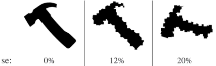
se: 0% 12% 20%

Fig. 2: Examples of various amount of segmentation errors (se). First an omnidirectional image without se, then the same test with se= 12%, lastly the same template from a perspective test case with se= 20%.

3 E

VALUATION ON SYNTHETIC DATA

For the quantitative evaluation of the proposed method, we generated different benchmark sets using 25 template shapes as 3D planar regions and their images taken by virtual cameras. The 3D data is generated by placing1/2/3 2D planar shapes with different orientation and distance in the 3D Euclidean space. Assuming that the longer side of a template shape is 1m, a set of 3D template scenes are obtained with 1/2/3 planar regions that have a random relative distance of ±(1−2)m between each other and a random relative rotation of±30^◦.

Both in the perspective and omnidirectional case, a 2D image of the constructed 3D scenes was taken with a virtual camera using the internal parameters of a real 3Mpx 2376× 1584 camera and a randomly generated absolute camera pose. The random rotation of the pose was in the range of ±40^◦ around all three axes. The random translation was given in the range ±(0.5 −2)m in horizontal and vertical directions and (2−6)m in the optical axis direction for the perspective camera, while the omnidirectional camera was placed at half the distance, i.e.

(1−3)m in the direction of the optical axis, and±(0.5−1)m in the X and Y axis directions to obtain approximately equal sized image regions for both type of cameras.

In practice, we cannot expect a perfect segmentation of the regions, therefore the robustness against segmentation errors was also evaluated on synthetic data (see samples in Fig. 2): we randomly added or removed squares distributed uniformly around the boundary of the shapes, both in the 2D images and on the edges of the 3D planar regions, yielding different levels of segmentation error expressed as the percentage of the original shape’s area. Using these images, we tested the robustness against 2D and 3D segmentation errors separately by performing a systematic series of tests using 1, 2, and 3 planes gradually increasing the segmentation error in each tests case individually. Based on these results we determined the noise level for each considered plane configurations such that the median rotation error around any of the axes remains under 1^◦ and we show combined error plots of these particular noise levels.

Theoretically, one single plane is sufficient to solve for the absolute pose, but it is clearly not robust enough. We have also found, that the robustness of the1-plane minimal case is also influenced by the shape used: Symmetric or less compact shapes with smaller area and longer contour,

and shapes with elongated thin parts often yield suboptimal results. However, such a solution can be used as an initialization for the solver with more regions. Adding one extra non-coplanar region increases the robustness by more than 4 times! This robustness enhancement quickly saturates with the number of regions, thus in our experiments we limited the number of non-coplanar patches to 3. We also remark, that the planarity of the regions is not strictly required. In fact, the equations remain true as long as the 3D surface has no self-occlusion from the camera viewpoint (see [4] for a cultural heritage application). Of course, planarity guarantees that the equations remain true regardless of the viewpoint.

Since the proposed algorithms work with triangulated 3D data, the planar regions of the synthetic 3D scene were triangulated. For the perspective test cases a plain Delaunay triangulation of only the boundary points of the shapes were used, thus the mesh contains less but larger triangles, which are computationally favorable. For the spherical solver, however, a higher number of evenly sized triangles is desirable for a good surface approximation, which was produced by thedistmesh2D function of [55] with the default parameters.

For a quantitative error measure, we used the rotation errors along the 3D coordinate axes as well as the overall rotation error as the rotation angle (or angular distance) ǫ = RRb ^⊤, R being the true rotation matrix and Rb the estimated one; and the difference between the ground truth tand estimatedˆttranslation vectors askt−ˆtk.

Furthermore, as a region-based back-projection error, we also measured the percentage of non-overlapping area (denoted by δ) of the reference 3D shape back-projected onto the 2D image plane and of the 2D observation image. The algorithms were implemented in Matlab and all experiments were run on a standard six-core PC. A demo implementation is available at http://www.inf.u-szeged.hu/

∼kato/software/ The average runtime of the algorithm varies from1−3seconds in the perspective case to4−7seconds in the omnidirectional case, without explicit code or input data optimization. Quantitative comparisons in terms of the various error plots are shown for each test case.

3.1 Omnidirectional cameras

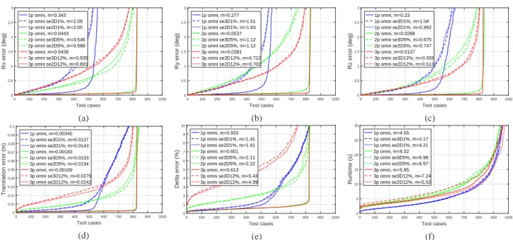
The results with 1, 2 and 3 non-coplanar regions using omnidirectional camera are presented in Fig. 3. In Fig. 3a - Fig. 3d, the rotation and translation errors for various test cases are presented. In the minimal case (i.e.1region), errors quickly increase, but using one more region stabilizes the solution: not only the error decreases but the number of correctly solved cases is also greatly increased. The δ error plot in Fig. 3e also confirms the robustness provided by more regions, while it has to be noted that with more regions the back-projection error does not improve in the way the pose parameter errors would imply, since even a smaller error in the pose yields larger non-overlapping area because of the longer boundary of the distinct regions. While using a second non-coplanar region brings

(8)

0 100 200 300 400 500 600 700 800 900 1000

Test cases 0

0.5 1 1.5 2 2.5 3

Rx error (deg)

1p omni, m=0.343 1p omni se3D1%, m=2.09 1p omni se2D1%, m=2.05 2p omni, m=0.0443 2p omni se3D5%, m=0.546 2p omni se2D5%, m=0.588 3p omni, m=0.0438 3p omni se3D12%, m=0.935 3p omni se2D12%, m=0.891

(a)

0 100 200 300 400 500 600 700 800 900 1000

Test cases 0

0.5 1 1.5 2 2.5 3

Ry error (deg)

(b)

0 100 200 300 400 500 600 700 800 900 1000

Test cases 0

0.5 1 1.5 2 2.5 3

Rz error (deg)

(c)

0 100 200 300 400 500 600 700 800 900 1000

Test cases 0

0.01 0.02 0.03 0.04 0.05 0.06 0.07 0.08 0.09 0.1

Translation error (m)

(d)

0 100 200 300 400 500 600 700 800 900 1000

Test cases 0

1 2 3 4 5 6 7 8 9 10

Delta error (%)

(e)

0 100 200 300 400 500 600 700 800 900 1000

Test cases 0

5 10 15 20 25 30

Runtime (s)

(f)

Fig. 3: Omnidirectional rotation errors along theX,Y, andZ axis (first row) and translation,δerror and runtime plots (second row).mdenotes median error, se2D and se3D stand for segmentation error on the 2D and 3D regions respectively (best viewed in color).

0 100 200 300 400 500 600 700 800 900 1000

Test cases

0 5 10 15 20 25 30

Runtime (s)

0 0.5 1 1.5 2 2.5 3 3.5 4 4.5 5

Delta error (%)

time, triang, m=4.05 time, pixelwise, m=71.8 delta, triang, m=0.933 delta, pixelwise, m=1.19

Fig. 4: Backprojection (δ) errors and runtime comparison for point and triangle based spherical surface integral approximation on a1 plane dataset (best viewed in color).

a rather big improvement, adding subsequent coplanar or non-coplanar regions yield only slight improvement over 2 regions. Fig. 8 shows the performance using 3 planes with 1 and 2 regions per plane, and 5 non-coplanar regions.

Practically the increase of the number of regions above 3 does not improve significantly the performance.

While the perfect dataset is solved with median translation errors as low as 2mm (see Fig. 3d), the error is increased by an order of magnitude, but still being under3cm, for regions corrupted with segmentation error. According to our previous experience [46], aδbelow5%corresponds to a visually good result. Combining this metric with the rotation error limit of 1^◦, we conclude that our method is robust against segmentation errors of up to ≈ 12% if at least 3non-coplanar regions are used.

We have experimentally shown that the size of the

spherical regions is greatly influencing the performance of the solver. While placing the camera closer to the scene produces larger spherical projections of the regions and the pose estimation becomes more robust, we aimed to use real world camera parameters instead, thus the camera-to-scene distance was limited. In our test cases, the median area of the spherical projections for the1and3 region cases were 0.07and0.13units respectively on the unit sphere.

For computing the spherical surface integrals, we compared two different approaches for the area approximation of the spherical regions. Our earlier approach is using standard numerical integration over the pixels projected onto the unit sphere [46], while the current one in Algorithm 1 is integrating over spherical triangles instead. Theδerror and runtime of these numerical schemes are compared in Fig. 4, which clearly shows that the CPU time of Algorithm 1 is an order of magnitude faster while the precision remains the same as for the earlier scheme in [46]. The slight precision change is caused by the pixel level discretization of the regions, since the triangulated shapes are generated using a subset of the boundary pixels, thus the triangles practically average out the rasterized edges to a smoother edge, making the integrals slightly more precise.

The algorithm’s CPU runtime is shown in Fig. 3f, where the slightly increased runtime of the 3D segmentation error test cases (noted by se3D) is due to the triangulation of the corrupted planar regions, that increases the number of triangles around the edges and thus the computational time.

Practically our algorithm can solve the pose estimation problem of an omnidirectional camera in≈5seconds using 2regions.

(9)

0 100 200 300 400 500 600 700 800 900 1000

Test cases 0

0.5 1 1.5 2 2.5 3

Rx error (deg)

1p pers, m=0.0772 1p pers se3D2%, m=1.24 1p pers se2D2%, m=0.986 2p pers, m=0.0205 2p pers se3D9%, m=0.659 2p pers se2D9%, m=0.686 3p pers, m=0.0155 3p pers se3D20%, m=0.872 3p pers se2D20%, m=0.979

(a)

0 100 200 300 400 500 600 700 800 900 1000

Test cases 0

0.5 1 1.5 2 2.5 3

Ry error (deg)

1p pers, m=0.0642 1p pers se3D2%, m=0.903 1p pers se2D2%, m=0.907 2p pers, m=0.0269 2p pers se3D9%, m=1.05 2p pers se2D9%, m=1 3p pers, m=0.014 3p pers se3D20%, m=0.848 3p pers se2D20%, m=0.921

(b)

0 100 200 300 400 500 600 700 800 900 1000

Test cases 0

0.5 1 1.5 2 2.5 3

Rz error (deg)

(c)

0 100 200 300 400 500 600 700 800 900 1000

Test cases 0

0.01 0.02 0.03 0.04 0.05 0.06 0.07 0.08 0.09 0.1

Translation error (m)

(d)

0 100 200 300 400 500 600 700 800 900 1000

Test cases 0

1 2 3 4 5 6 7 8 9 10

Delta error (%)

(e)

0 100 200 300 400 500 600 700 800 900 1000

Test cases 0

5 10 15 20 25 30

Runtime (s)

(f)

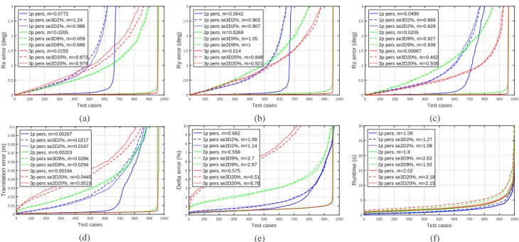
Fig. 5: Perspective pose estimation results: rotation and translation errors, δ error and algorithm runtime plots. se2D stands for observation segmentation error, se3D for template side segmentation error and m for median values (best viewed in color).

0 100 200 300 400 500 600 700 800 900 1000

Test cases

0 1 2 3 4 5 6 7 8 9 10

Delta error (%)

1p pers, m=0.662 1p pers-sph, m=2.64 2p pers, m=0.556 2p pers-sph, m=0.587 3p pers, m=0.575 3p pers-sph, m=0.667

Fig. 6: Perspective pose estimation δ errors comparing the normalized image plane and the spherical solutions. m stands for median values (best viewed in color).

0 100 200 300 400 500 600 700 800 900 1000

Test cases

0 5 10 15 20 25 30

Runtime (s)

1p pers, m=1.09 1p omni, m=4.05 1p pers-sph, m=32.9 2p pers, m=1.8 2p omni, m=6.02 2p pers-sph, m=37.2 3p pers, m=2.02 3p omni, m=5.95 3p pers-sph, m=29.5

Fig. 7: Runtime comparison on test cases without segmentation errors in the omnidirectional and perspective case, the latter using both the normalized image plane and the spherical solution. m stands for median values (best viewed in color).

0 10 20 30 40 50 60 70 80 90 100

Test cases

0 0.5 1 1.5 2 2.5 3

Rotation error ǫ (deg)

3p omni, m=0.058 3p6reg omni, m=0.0572 5p omni, m=0.0511 3p omni se3D12%, m=1.36 3p6reg omni se3D12%, m=1.75 5p omni se3D12%, m=1.28 3p omni se2D12%, m=1.26 3p6reg omni se2D12%, m=1.74 5p omni se2D12%, m=1.43

0 10 20 30 40 50 60 70 80 90 100

Test cases

0 0.5 1 1.5 2 2.5 3

Rotation error ǫ (deg)

3p pers, m=0.0253 3p6reg pers, m=0.0237 5p pers, m=0.0219 3p pers se3D20%, m=1.42 3p6reg pers se3D20%, m=1.49 5p pers se3D20%, m=1.22 3p pers se2D20%, m=1.46 3p6reg pers se2D20%, m=1.47 5p pers se2D20%, m=1.41

Fig. 8: Overall rotation error in function of the number of regions and planes for the omnidirectional (top) and perspective (bottom) camera. m stands for median values (best viewed in color).

(10)

0162-8828 (c) 2019 IEEE. Personal use is permitted, but republication/redistribution requires IEEE permission. See http://www.ieee.org/publications_standards/publications/rights/index.html for more 3.2 Perspective cameras

Pose estimation results using a perspective camera are presented in Fig. 5, including the same test cases with1, 2and3non-coplanar regions and with segmentation errors as in the omnidirectional case. The rotation and translation error plots in Fig. 5a - Fig. 5d clearly confirm the advantage of having more non-coplanar regions.

The median translation error (see Fig. 5d) on the perfect dataset is as low as2mm, which increases by an order of magnitude in the presence of 20%segmentation error, but still being under 5cm in case of 3 regions. The δ error plot in Fig. 5e also shows the robustness provided by the additional regions. Obviously, the back-projection error also increases in the presence of segmentation errors. However, as Fig. 5a - Fig. 5d shows, the actual pose parameters are considerably improved and the robustness greatly increases by using1 or 2 extra non-coplanar regions. Similar to the omnidirectional case, the increase of the number of regions above 3 does not improve significantly the performance of the pose estimation (see also Fig. 8).

The algorithm’s CPU time on perspective test cases is shown in Fig. 5f. The increased runtime of the 3D segmentation error test cases (noted by se3D) is due to the triangulation of the corrupted planar regions, that greatly increases the total number of triangles and thus the computational time. Practically our algorithm can solve the pose estimation problem of a perspective camera in around 2.5 seconds using2 regions.

As mentioned in Section 2.2, a perspective camera can also be represented by the spherical model developed in Section 3.1. However, as we have shown in the previous section, this model’s main limitation is the small size of the spherical regions, because a perspective camera has a narrower field of view and has to be placed at a larger distance from the scene, to produce the same size of regions on the image. The resulting spherical projections of the planar regions in median are typically 4 times smaller than in the omnidirectional camera’s case. Thus solving the perspective case using the spherical solver yields a degraded performance, as shown by the δ error plot in Fig. 6. Comparing the algorithm’s runtime plot in Fig. 7 also shows that using the spherical solver for the perspective camera greatly increases the computing time due to the calculation of surface integrals on the sphere, which confirms the advantage of using the perspective solver proposed in Section 2.2, instead of a unified spherical solver.

3.3 Degeneracy analysis

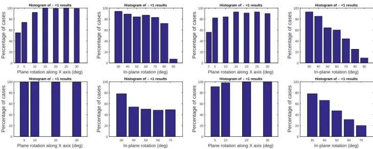
In order to analyze the degeneracy characteristics of the proposed method, two separate tests were performed: one along the X axis rotation (rotations along the Y axis would have similar effects) and another one for the in- plane rotation (along the Z axis). Both test cases are also linked to the robustness of the initialization step of the algorithm. For these experiments, a series of new datasets with 100 test cases each were generated using one region

with non-symmetric template shapes (symmetric ones were considered separately).

In each dataset, R_X was set to a fixed absolute value such that the viewing angle between the plane and the camera optical axis was ranging from 50^◦ down to 2^◦ in steps of 5^◦, yielding gradually increased perspective distortions up to the extreme 2^◦ case. The other rotation parameters were set to 0, and the translation along the optical axis was randomly generated to ensure roughly equally sized projections on the image plane. This is needed to a correct evaluation where results are not influenced by other pose parameters or the changes in the size of the projected regions. Experimental results in Fig. 9 show that if the camera’s orientation is initialized within±60^◦ of the true rotation (i.e. a quite rough initialization suffices), the algorithm can robustly find the correct solution even in case of degenerate viewing angles: at least80%of the cases are solved withǫ <1^◦rotation error forR_X>= 5^◦, but below 5^◦viewing angle, the errors increase significantly. Symme- try of the template shapes doesn’t affect significantly the results, since the projectively distorted shapes usually don’t preserve the symmetry.

Degeneracy analysis along theZ axis (in-plane rotations only) practically translates into the initialization problem of the in-plane rotation, which can be performed in a real application using a rough estimate of e.g. the vertical direction. As in the previous case, we generated our datasets with a pureR_Z rotation around theZ axis going from30^◦ to90^◦in absolute value, while setting all other rotations to 0 and the translation along the optical axis was randomly generated to ensure roughly equally sized projections on the image plane. Since the initialization of R_Z = 0 was used throughout the test cases, these rotations directly translate into a rotation error in the initialization of R_Z. Experimental results show, that if the in-plane rotation is initialized within a±60^◦ (±80^◦ for the perspective) of the true rotation, the proposed method robustly finds a correct solution (conditioned to the use of non-symmetrical shapes) as this is visible in the second and last histogram plots of Fig. 9. In contrast to the plane rotation alongXandY axes, the in-plane rotation preserves the symmetry of the template shapes in our setup, thus results are greatly affected if symmetric shapes are used, but30^◦−40^◦initialization error is easily tolerated even for symmetric shapes.

4 E

VALUATION ON REAL DATASETS

To thoroughly evaluate our method on real world test cases, we used several different 3D data recorded by commercial as well as a custom built 3D laser range finder with corresponding 2D color images captured by commercial SLR and compact digital cameras with prior calibration and radial distortion removal. Whatever the source of the 2D-3D data is, the first step is the segmentation of planar region pairs used by our algorithm. There are several automated or semi-automated 2D segmentation algorithms in the literature including e.g. clustering, energy-based or region growing algorithms [56]. In this work, a simple