Comparison of Mono Camera-based Static Obstacle Position Estimation Methods for Automotive Application
Peter Bauer1, Antal Hiba2, Akos Zarandy2
Abstract— This paper presents the comparison of four dif- ferent mono camera-based steady obstacle position and size estimation algorithms focusing on automatic emergency braking application. Three methods are well known in the automotive field, the fourth is the author’s own method successfully applied in aerospace until now. The first contribution is the extension of all methods to consider multiple data points and variable velocity (where possible). The second contribution is an extensive simulation testing of the methods considering constant and variable speeds, attitude uncertainties and the braking characteristic of real vehicles. The methods are evaluated based- on the worst case hitting speed of the obstacle and the precision of obstacle side distance and size estimation. The maximum speeds of applicability are determined for all methods and the results are commented in detail.
I. INTRODUCTION
In the past decades automotive systems approach higher and higher levels of autonomy starting with cruise control (CC) until the first Level 2 autopilot systems (such as Tesla autopilot). In these systems several tasks require the estima- tion of distance and speed of the obstacles and vehicles ahead and current systems have limitations in their operational range regarding the own vehicle speed. Currently EuroNCAP tested ten vehicles equipped with driver assistance systems (see [1]) and experienced that there are several limitations and user alert and intervention were required several times.
Regarding stopping before a stationary target at 50km/h all systems performed well and stopped meanwhile at 80km/h six systems failed out of the ten. This means that there is a possibility and need for developments even considering stationary obstacles.
The author targets to compare existing mono camera-based methods without radar assistance as this is an extensively researched field in automotive ([2],[3],[4],[5],[6],[7],[8],[9],[10],[11]) and a good opportunity to evaluate his mono camera-based obstacle avoidance algorithm ([12],[13]) used in aerospace until now. The final goal is to select the best algorithm which can be further evaluated and possibly tested in automotive application.
This paper was supported by the J´anos Bolyai Research Scholarship of the Hungarian Academy of Sciences. The research presented in this paper was funded by the Higher Education Institutional Excellence Program.
1author is with Systems and Control Laboratory, Institute for Computer Science and Control, Hungarian Academy of Sciences, H-1111 Budapest, Kende utca 13-17, Hungarybauer.peter@sztaki.mta.hu
2author is with Computational Optical Sensing and Processing Labora- tory, Institute for Computer Science and Control, Hungarian Academy of Sciences, H-1111 Budapest, Kende utca 13-17, Hungary
Part of the literature sources consider fiducial markers with known size such as license plates [5], [7] and artificial tags [4]. The problem with small markers is their detectability from larger distances as [3] points out (above 30m its hard to detect them) and the possible change of size in different countries. Other sources assume known lane width or vehicle size such as [3], [8]. The problem here is that several different vehicle widths and lane widths [14] can be observed so such methods can give uncertain results. That’s why known size based methods are not considered in this study.
Scale change of the obstacle image and system sampling time are considered in [6] and [11] to estimate time to collision (TTC). Assuming known constant velocity the range of the obstacle can be estimated and with known range the size and side distance can also be estimated as pointed out in subsection III-A. This is the first method considered in comparison and denoted by SC (scale-based).
Scale change and traveled distance are considered in [10]
from which the range and again the size and side distance can be determined. As the traveled distance is measurable through odometer and GPS this is the second method con- sidered as SCD (scale and distance-based).
Point of contact of the vehicle with ground and known camera height are considered in [2], [8] from which the range can be directly obtained and again the size and side distance.
This is the third tested method as G (ground-based).
The fourth method is the author’s aerospace method [12]
which considers scale change with constant velocity [13]
and estimates TTC and the closest point of approach (CPA) which is the ratio of side distance and obstacle width. It is denoted by SAA (originally aircraft sense and avoid).
Its worth to mention that some sources use Kalman filtering to smooth results ([9], [8]) but such methods will be targeted in another work after detailed comparison of the basic methods here.
Besides comparison the contribution of this work is to present the selected four methods on a common basis and extend them to the use ofN data samples and time-varying speeds where possible. The further structure of the paper is as follows: section II introduces the considered simulation setup, test scenarios and the evaluation method of the test results. Section III describes the selected four methods and extends them where possible, section IV evaluates the results of the test campaign and finally section V concludes the paper.
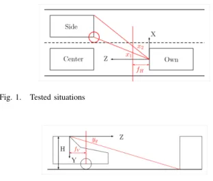
II. TEST SCENARIOS AND EVALUATION The simulated test scenario is the approach of a static obstacle (vehicle) either in the own lane or in the neighboring one as shown in Fig. 1. So either the center lines of the vehicles are aligned (center case) or there is one lane width difference between them (on the right side of the own, side case). The considered vehicle widths in lane design are 1.75m for car and 2.55m for truck as shown in [14]
and a typical lane width can be 3m. These parameters are considered in the simulations. A straight flat road without slopes and curves is assumed.
A pinhole camera projection model was applied consider- ing thefH= 1373pxandfV = 1925pxfocal lengths of the Bosch MPC2 automotive camera and pixelization errors. The camera is assumed to be aligned with the center line of the own vehicle with coordinate axes Z forward and horizontal, X rightward, Y downward. The considered image parameters are thex1left corner of obstacle,S=x2−x1size (see Fig.
1) and yg ground contact point (see Fig. 2). Side position estimation targets the position of the obstacle left corner (see Fig. 1). Cameraf psis assumed to be 10 as a realistic value with onboard systems.
Fig. 1. Tested situations
Fig. 2. Side view with ground contact point
The simulated scenarios include constant speed approach of the obstacle between 20 and 130km/h, variable speed approach which means a sinusoidal variation of the lon- gitudinal speed and addition of a sinusoidal lateral speed component and ramp up/down (between 20 and 130km/h) speed approach. Additionally, pitch or yaw angle sinusoidal disturbances were applied to test the camera angular align- ment sensitivity of the methods. Vehicle speed and position were assumed to be perfectly known at every time step in the implementation of the algorithms.
The added longitudinal velocity disturbance is: ∆Vz = 1.34 sin 2πT +π2
[m/s] with T = 3sec period time while the lateral is:∆Vx= 0.4 sin 2πT +π2
[m/s]. The amplitude of the former was determined considering the 9-10sec speed up of an average car from 0 to 100km/h which means about2.8m/s2acceleration. The amplitude of the latter was determined to give about 0.4m maximum side motion of the own vehicle which can be realistic inside the lane.
The pitch angle disturbance is given as∆θ= 1 sin 2πZ10 so it is distance dependent as the pitching caused by road errors and its amplitude is 1◦. The yaw disturbance is the same when applied.
As the main attempt is to evaluate the methods regarding emergency braking the braking distance of the own vehicle from different speeds should be considered. A braking model is set up in [15] giving the jerk asaa =−20m/s3 and the brake system delay ast2= 0.18s. A more detailed braking model is used in [16] as: S = (t1+t2+ 0.5t3)V0+ 2aV02 including t1 as driver reaction time, t3 as decelerationx
increase time andaxas settled deceleration (V0 is the initial speed). Considering automatic emergency braking the t1
driver reaction time can be neglected and only the other times considered. The braking model in [16] was modified to have three parts: distance traveled during system delay S2 = V0t2, distance traveled until deceleration builds up S3 = V0t3 +aa
t33
6 and distance traveled during constant decelerationS4=V3t4+ax
t24
2. The settled deceleration was selected to beax=−7.6m/s2as the general case in [16].t3
is either the time until standstillt3lim=q
2V0
|aa| or the time until deceleration settles t3 = aax
a whichever achieved first.
V3 = V0+aat23
2 is the speed achieved during deceleration build up. t4 = |aV3
x| is the time until standstill. The overall braking distance results asS=S2+S3+S4+ 1where the last term 1mis a targeted safety distance from the obstacle at standstill. This S distance is calculated between 20 and 130km/h and the method of system evaluation is to check if the estimated obstacle distance Zˆ is below S. This case emergency braking should be initiated and the difference of the real distance Z and the braking one S at this time gives the final distance between obstacle and own vehicle
∆S=Z−S.∆S >0 means successful stop before hitting the obstacle. Difference of estimated and real obstacle size and side distance are also calculated and compared at this time.
The evaluation criteria for the methods was set as below:
• Size or side position estimation is acceptable if the error is in the±0.2mrange. With this error range assuming at least 0.6m targeted distance between vehicles in case of an avoidance maneuver the worst case distance on the left side will be 0.4m while on the right 0.2m.
• Considering the 50km/h test speed with full width rigid barrier of Euro NCAP [17] the obstacle hitting speed in case of non-complete stop can safely be allowed to be 20 or 30km/h (probability of severe injury very low). 20km/h hitting speed means 2m remaining braking distance∆S≥ −2, while 30km/h means 4.57m ∆S≥
−4.57.
• Methods are evaluated based-on the satisfaction of the 20km/h (Limit20 or Lim20) or 30km/h (Limit30 or Lim30) braking distance limit together with the accept- able estimation of size and side position. The highest speed at which all limits are satisfied is chosen as the limit of applicability of the given method in the given scenario. Detailed test results are summarized in Section
IV.
III. OVERVIEW OF METHODS
Methods referenced in the introduction are collected here and extended to use N data points to smooth results and consider time-varying velocity if possible. At first, all meth- ods are presented for constant velocity then the extensions are described.
A. Time to collision from scale change (SC)
Probably the simplest method is the one published in [6].
This estimates TTC from the scale change of the obstacle size in the camera and the sampling time (∆t) (f ps of camera) as follows:
T T Cˆ k= ∆t Sk−1
Sk−Sk−1 (1) From the TTC estimate the absolute distance, side distance and real size can be estimated with known longitudinal velocityVz:
Zˆk=VzT T Cˆ k, Xˆ0= 1
fHxkZˆk, Wˆ = 1
fHSkZˆk (2) This TTC estimation method can be easily extended to considerN data samples as:
T T Cˆ k = (N−1)∆t Sk−N+1 Sk−Sk−N+1
(3) Considering a longer horizon can suppress high errors caused by sudden local changes. Unfortunately, the case of time-varying velocity can not be included into this frame- work as it does not comply with TTC estimation.
B. Distance from scale change and traveled distance (SCD) This method is published in [10]. Knowing the image coordinates of a point on the object at two time steps xk−1, yk−1 andxk, yk and the traveled 3D distances during that time Tx(k−1) = Xk −Xk−1, Ty(k−1) = Yk − Yk−1, Tz(k−1) =Zk−Zk−1 one can obtain the system of equations below from the pinhole camera projection model.
Assuming Ty(k−1) = 0 (no vertical displacement) the system can be further simplified.
xk
yk
=
"fH(Xk−1+Tx(k−1))
Zk−1+Tz(k−1) fV(Yk−1+Ty(k−1))
Zk−1+Tz(k−1)
#
=
Zk−1 Zk−1+Tz(k−1)
"
fH Xk−1
Zk−1
fVYZk−1
k−1
#
| {z }
hxk−1 yk−1iT +
fH Zk−1+Tz(k−1)
Tx(k−1) 0
(4)
Extension of this method to N data points and variable velocity is straightforward as points further in time can be
considered and the traveled distances can be calculated from the related positions.
xk
yk
= Zk−N+1
Zk−N+1+Tz(k−N+ 1)
| {z }
s1
xk−N+1 yk−N+1
+
fH
Zk−N+1+Tz(k−N+ 1)
| {z }
s0
Tx(k−N+ 1) 0
Tx(k−N+ 1) =Xk−Xk−N+1
Tz(k−N+ 1) =Zk−Zk−N+1
(5)
If one can determine s1, s0 than the distance Zk = Zk−N+1+Tz(k−N+ 1)can be determined with them:
Zˆk = s1Tz(k−N+ 1)
1−s1 +Tz(k−N+ 1) Zˆk = fH−s0Tz(k−N+ 1)
s0
+Tz(k−N+ 1) (6)
s1, s0 can be determined from a system of equations:
xk
yk
=
xk−N+1 Tx(k−N+ 1)
yk−N+1 0
s1
s0
(7) IfTx(k−N+ 1)is close to zero than the matrix is close to singular so its better to solve the 2 equations only fors1 and then average:
ˆ s1=1
2 xk
xk−N+1 + yk
yk−N+1
(8) After determining Zˆk Wˆ and Xˆ0 can be determined similarly as in (2). A possible problem with this method is thatxcan be yaw andy can be pitch sensitive. This will be examined during the tests.
C. Distance estimation based-on ground contact point (G) This method is described in [2]. It is based-on the known height of the camera mounted on the own car H and the vertical coordinate of the ground contact point of the obstacle in the camera image ygk (see Fig. 2). The distance can be directly calculated from them:
Zˆk =fVH
ykg (9)
After determining Zˆk Wˆ and Xˆ0 can be determined similarly as in (2). This method does not include any assump- tion about the speed so time-varying speed does not cause problem. However, it is very sensitive to the pitching motion of the car (if it is not compensated). Possibly some smoothing can be applied by considering the traveled distance and solving a system of equations by simply averaging the left hand side forZˆk:
fVH ygk fVH
yk−1g +Tz(k−1) ...
fVH
yk−N+1g +Tz(k−N+ 1)
=
1 1 ... 1
Zˆk (10)
D. Method based-on TTC and CPA estimation (SAA) This method was developed by the author for aircraft sense and avoid application as published in [12] and [13]. The basic formulas relate forward (Z) and side distances (X) and the object size (W) to the measurable image parameters (x,S):
1 Sk
= Zk fHW, xk
Sk
= Xk
W (11)
Considering Vx = 0 side velocity (Xk = X0 =const), Vz<0forward velocity and the camera projection model in Fig. 1:
1 Sk
=− Vz
fHWT T Ck= Vz fHW
| {z }
a
tk− Vz fHWtC
| {z }
b
xk Sk
=CP A
(12)
The first expression gives a possibility to fit line on the points1/Sk, tk and so obtain the absolute time of collision astC =−b/aandT T Cˆ k=tC−tk. At least two points are required to do this but more points will give better results as the tests will show.CP Aˆ =XW0 can be simply calculated as the average of thexk/Sk ratios.
Extension of this method to time-varying speed is possible but requires a completely different solution method. With time-varying speed the distances can be calculated as follows (Z0, X0 initial distances):
Z=Z0+ Z t
t0
Vzdt, X=X0+ Z t
t0
Vxdt (13) Substituting these into (11) and grouping the known and unknown terms gives the following system of equations:
1 Sk = 1
fH Z0
W + Rtk
t0 Vzdt fH
1 W xk
Sk
= 1 X0
W
|{z}
CP A
+ Z tk
t0
Vxdt 1 W
(14)
This system of equations includes three unknown constant parameters Z0/W,1/W, CP A. It is advisable to multiply the first equation with fH to make it better conditioned and to solve it first for Z0/W,1/W considering multiple measured points. Then CPA can be determined from the second equation with known1/W and averaging if multiple points are considered. Finally, the side distance can be calculated asX0=CP A·W
IV. TEST RESULTS
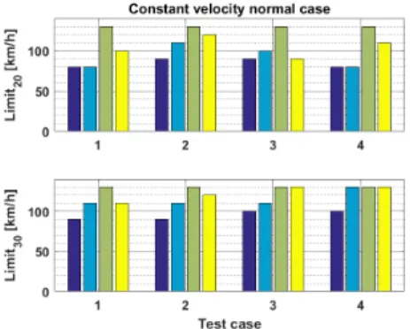
First, the applicability of the constant velocity formulas was tested simulating constant vehicle speed. Beside the normal undisturbed case (see Fig. 3) cases with pitch (see Fig. 4) and yaw (see Fig. 5) disturbances are also considered to estimate sensitivity to small angular errors (1◦disturbance only). The figures show the limit speeds of applicability of each method as bar plots. Numbers on the horizontal axis belong to 1 = car/center, 2 = truck/center, 3 = car/sideand4 =truck/sideevaluated scenarios. Four bars are plotted for every scenario representing respectivelySC, SCD, G and SAA methods. The 5km/h bar value means that the method is not applicable even for 20km/h vehicle speed. The overall summary of applicability limits is given in Table I.
Fig. 3. Constant velocity normal test case
Fig. 4. Constant velocity pitch disturbance test case
Fig. 5. Constant velocity yaw disturbance test case
Table I shows that in the normal case the best is the G method applicable at the 130km/h maximum test speed also. The second best is the SAA method applicable until 110km/h with the 30km/h hitting speed limit. However, considering the really small 1◦ pitch disturbance the G method becomes inapplicable while the SAA method still performs well with slightly decreased 100km/h speed limit.
This case the performance of the SC method is also ac- ceptable. This result is not surprising as SC and SAA methods do not use the y coordinate which is disturbed by pitching. Considering the small yaw disturbance the SCD method becomes inapplicable and the applicability of SC and G become severely limited while the limits for the SAA method stay the same as for the pitch case. The G method is limited only by the side distance estimate the forward distance and obstacle size estimates are as good or better than with SAA. The side distance from SAA is calculated in a different way (X0 = CP A· W) so this can cause the difference. As a summary, it can be stated that the SAA method outperforms the others if there is a possibility of angular disturbances which is the usual case for moving vehicles even with attitude angle compensation as its precision is rarely below 1◦.
TABLE I
FINAL COMPARISON OF CONSTANT VELOCITY TEST RESULTS
Test case Limit SC SCD G SAA
CONST normal Lim20 80 80 130 90
Lim30 90 110 130 110
CONST pitch Lim20 80 20 N/A 90
Lim30 80 20 N/A 100
CONST yaw Lim20 30 N/A 30 90
Lim30 30 N/A 30 100
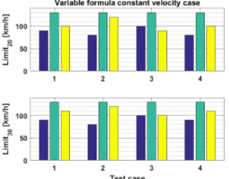
Second, the applicability of the variable velocity formulas was tested simulating variable vehicle speed. Beside the normal undisturbed case (see Fig. 6) cases with pitch (see Fig. 7), yaw (see Fig. 8) and pitch and yaw disturbances are also considered to estimate sensitivity to small angular errors (1◦ disturbance only). The pitch and yaw plot is very similar to the pitch one with slightly different numerical values which are shown in Table II. Here an extra case is the application of the variable speed formulas with constant vehicle speed in Fig. 9 as this is a realistic situation with such system. The concept of figures is the same as for the constant velocity, but only three bars are plotted for every scenario representing respectivelySCD,GandSAAas the SC case was not applicable for variable speed. The overall summary of applicability limits is given in Table II.
TABLE II
FINAL COMPARISON OF VARIABLE VELOCITY TEST RESULTS
Test case Limit SCD G SAA
VAR normal Lim20 60 130 90
Lim30 60 130 90
VAR pitch Lim20 N/A N/A 90
Lim30 N/A N/A 90
VAR yaw Lim20 N/A 50 70
Lim30 N/A 50 100 VAR pitch/yaw Lim20 N/A N/A 70
Lim30 N/A N/A 100
VAR CONST Lim20 80 130 90
Lim30 80 130 100
Fig. 6. Variable velocity normal test case
Fig. 7. Variable velocity pitch disturbance test case
Fig. 8. Variable velocity yaw disturbance test case
Table II shows that in the normal case the best is the G method applicable at the 130km/h maximum test speed
also. The second best is the SAA method applicable un- til 90km/h. Regarding the disturbed cases method SCD becomes inapplicable for any angular disturbance and its original applicability with 60km/h limit is also low. From the G and SAA methods the latter better preserves its applicability giving at least 70km/h limit speed for any applied disturbance and a maximum of 100km/h in some cases. Here, again theGmethod is limited only by the side distance estimate in the yaw disturbance case the forward distance and obstacle size estimates are as good or better than with SAA. Considering the constant velocity test scenario again Gis the best andSAA is only the second best. As a summary, it can be stated that theSAAmethod outperforms the others if there is a possibility of angular disturbances which is the usual case for moving vehicles.
Fig. 9. Variable velocity formula constant velocity test case
All of the test result were generated with N = 10 data samples (1s data) per step, but the constant normal cases were tested also with N = 5 and N = 2. In most of the cases there was performance degradation even withN = 5 so N= 10should be applied when possible.
Another test was the evaluation of variable speed formulas with ramp up (20 to 130km/h) or down (130 to 20km/h) vehicle speed profile reaching the end value at the obsta- cle. Regarding the estimated size and position all methods performed acceptable in every case (scenarios from 1 to 4).
Regarding the braking distance SCD was uncertain while G andSAA performed equally well satisfying the 20km/h hitting speed requirement in all cases.
V. CONCLUSIONS
This paper presents the comparison of four methods ca- pable to estimate the distance, position and size of a steady obstacle from monocular images. Three of them is from the automotive literature one is the author’s own method applied in aerospace.
The first contribution of the paper is to extend the methods to considerNdata points and variable velocity, however only three methods could be extended for variable velocity.
The second contribution is to run a lot of simulation tests considering car or truck obstacle in the own or in the neighbor lane and approaching them with different speeds and deciding the time of required emergency braking. Con- stant and variable (sinusoidal and ramp) speeds were all
considered in the range of 20 to 130 km/h. All cases were also tested with pitch and/or yaw angle disturbance to test the sensitivity of the methods to attitude disturbances (or camera misalignment). The evaluation criteria was the hitting speed of the obstacle (if the emergency braking does not stop completely the own vehicle because of estimation errors) and the precision of side distance and size estimation. The highest approach speed with which all defined thresholds are satisfied becomes the maximum applicability speed of each method.
The overall conclusion form the test campaign is that the own SAA method is the most reliable considering also the attitude disturbances which are inevitable with vehicles and even a good attitude compensation system can left1◦ error in the parameters. The other methods become unreliable with either pitch and/or yaw disturbance. The applicability limits of the own method are 90km/h for 20km/h and 100km/h for 30km/h hitting speed limit with the constant velocity formulas, which decreases to 70km/h and 90km/h in the variable speed cases respectively.
Future work should include closed form sensitivity analy- sis of the methods to underline these results, consideration of measurement errors regarding velocity and vehicle position and the extension of the methods for moving obstacle if possible.
REFERENCES
[1] (2018). [Online]. Available: https://www.euroncap.com/en/vehicle- safety/safety-campaigns/2018-automated-driving-tests/
[2] G. P. Stein, O. Mano, and A. Shashua, “Vision-based acc with a single camera: bounds on range and range rate accuracy,” inIEEE IV2003 Intelligent Vehicles Symposium. Proceedings (Cat. No.03TH8683), June 2003, pp. 120–125.
[3] R. Kanjee, A. K. Bachoo, and J. Carroll, “Vision-based adaptive cruise control using pattern matching,” in 2013 6th Robotics and Mechatronics Conference (RobMech), Oct 2013, pp. 93–98.
[4] P. Irmisch, “Camera-based distance estimation for autonomous vehicles,” Master’s thesis, Technische Universit¨at Berlin, December 2017. [Online]. Available: https://elib.dlr.de/116211/
[5] S. Chen and R. Chen, “Vision-based distance estimation for multiple vehicles using single optical camera,” in2011 Second International Conference on Innovations in Bio-inspired Computing and Applica- tions, Dec 2011, pp. 9–12.
[6] S. Gonner, D. Mullert, S. Hold, M. Meutert, and A. Kummert,
“Vehicle recognition and ttc estimation at night based on spotlight pairing,” in2009 12th International IEEE Conference on Intelligent Transportation Systems, Oct 2009, pp. 1–6.
[7] V. Karagiannis, “Distance estimation between vehicles based on fixed dimensions licence plates,” Master’s thesis, University of Patras, 02 2017.
[8] K. Nakamura, K. Ishigaki, T. Ogata, and S. Muramatsu, “Real- time monocular ranging by bayesian triangulation,” in 2013 IEEE Intelligent Vehicles Symposium (IV), June 2013, pp. 1368–1373.
[9] U. Franke and C. Rabe, “Kalman filter based depth from motion with fast convergence,” in IEEE Proceedings. Intelligent Vehicles Symposium, 2005., June 2005, pp. 181–186.
[10] A. Wedel, U. Franke, J. Klappstein, T. Brox, and D. Cremers,
“Realtime depth estimation and obstacle detection from monocular video,” inPattern Recognition, K. Franke, K.-R. M¨uller, B. Nickolay, and R. Sch¨afer, Eds. Berlin, Heidelberg: Springer Berlin Heidelberg, 2006, pp. 475–484.
[11] E. Dagan, O. Mano, G. P. Stein, and A. Shashua, “Forward collision warning with a single camera,” inIEEE Intelligent Vehicles Sympo- sium, 2004, June 2004, pp. 37–42.
[12] P. Bauer, A. Hiba, B. Vanek, A. Zarandy, and J. Bokor, “Monocular Image-based Time to Collision and Closest Point of Approach Estima- tion,” inIn proceedings of 24th Mediterranean Conference on Control and Automation (MED’16), Athens, Greece, 2016.
[13] P. Bauer, B. Vanek, and J. Bokor, “Monocular Vision-based Aircraft Ground Obstacle Classification,” in In Proc. of European Control Conference 2018 (ECC 2018), 2018, pp. 1827–1832.
[14] (2018). [Online]. Available: https://en.wikipedia.org/wiki/Lane [15] E. Coelingh, A. Eidehall, and M. Bengtsson, “Collision warning with
full auto brake and pedestrian detection - a practical example of automatic emergency braking,” in13th International IEEE Conference on Intelligent Transportation Systems, Sep. 2010, pp. 155–160.
[16] N. Kudarauskas, “Analysis of emergency braking of a vehicle,”
Transport, vol. 22, no. 3, pp. 154–159, 2007. [Online]. Available:
https://www.tandfonline.com/doi/abs/10.1080/16484142.2007.9638118 [17] (2019). [Online]. Available: https://www.euroncap.com/en/vehicle-
safety/the-ratings-explained/adult-occupant-protection/