arXiv:1609.02196v1 [math-ph] 7 Sep 2016
Conformal covariance and the split property
Vincenzo Morinelli
∗, Yoh Tanimoto
†Dipartimento di Matematica, Universitá di Roma Tor Vergata Via della Ricerca Scientifica, 1, I-00133 Roma, Italy email: morinell@mat.uniroma2.it, hoyt@mat.uniroma2.it
Mihály Weiner
‡Mathematical Institute, Department of Analysis, Budapest University of Technology & Economics (BME)
Műegyetem rk. 3-9, H-1111 Budapest, Hungary email: mweiner@math.bme.hu
Abstract
We show that for a conformal local net of observables on the circle, the split property is automatic. Bothfullconformal covariance (i.e. diffeomorphism covariance) and the circle-setting play essential roles in this fact, while by previously constructed examples it was already known that even on the circle, Möbius covariance does not imply the split property.
On the other hand, here we also provide an example of a local conformal net living on the two-dimensional Minkowski space, which — although being diffeomorphism covariant — does not have the split property.
1 Introduction
More than half a century passed away since the first formulation of an axiomaticquan- tum field theory. There are several existing different settings (differing e.g. on the chosen spacetime, or whether their fundamental notion is that of aquantum fieldor alocal observ- able) with many “additional” properties that are sometimes included among the defining axioms. For an introduction and overview of the topic we refer to the book of Haag [24].
∗Supported by the ERC advanced grant 669240 QUEST “Quantum Algebraic Structures and Models”.
†Supported by the JSPS fellowship for research abroad.
‡Supported in part by the ERC advanced grant 669240 QUEST “Quantum Algebraic Structures and Models” and by OTKA grant no. 104206.
Whereas properties likelocalityare unquestionably among the basic axioms, some other properties are less motivated and accepted. Haag-duality has an appealing mathematical elegance, but there seems to be no clear physical motivation for that assumption. Techni- calities, like the separability of the underlying Hilbert space are sometimes required with no evident physical reason.
The split propertyis the statistical independence of local algebras associated to regions with a positive (spacelike) separation. It might be viewed as a stronger version of locality, and contrary to the previous two examples, it was formulated on direct physical grounds.
However, traditionally it is not included among the defining axioms, as in the beginning it was unclear how much one can believe in it. Indeed, many years passed till this stronger version of locality was first established at least for the massive free field by Buchholz [2].
Only after the introduction of the nuclearity condition (which was originally motivated by the need of a particle interpretation [25]) it became more of a routine to verify the split property in various models, when its connection to nuclearity was discovered [6]. Another important step was the general mathematical understanding of split inclusions brought by the work of Doplicher and Longo [15].
In the meantime, interest rose in conformal quantum field theories, especially in the low dimensional case; i.e. conformal models given on the 2-dimensional Minkowski space and their chiral components that can be naturally extended onto the compactified lightray, the circle. The theory of conformal net of local algebras on S1 is rich in examples and it provides an essential “playground” to people studying operator algebras as it turned out to have incredibly deep connections to the modular theory of von Neumann algebras as well as to subfactor theory; see e.g. [19, 41, 29]. In particular, the modular group associated to a local algebra and the vacuum vector always acts in a certain geometric manner: the so-called Bisognano-Wichmann property is automatic. In turn, this was used to conclude that several further important structural properties — e.g. Haag-dualityand Additivity — are also automatic in this setting. We refer to the original works [19, 18, 1, 4] for more details on this topic.
The case of the split property seemed to be different — but there is an important detail to mention here. Initially, when studying chiral conformal nets, in the so-far cited works only Möbius covariance was exploited. There were several reasons behind this choice. First, because it is a spacetime symmetry implemented by a unitary representation for which the vacuum is an invariant vector. This is exactly how things go in higher dimension, but this is not how diffeomorphism covariance is implemented (no invariant vectors and one is forced to consider projective representations rather than true ones). Second, because the mentioned connection to modular theory of von Neumann algebras relies on Möbius covariance only. Thus, the listed structural properties — with the exception of the split property — are already automatic even if diffeomorphism covariance is not assumed.
From the physical point of view, however, diffeomorphism covariance is natural in the low dimensional conformal setting; by an argument of Lüscher and Mack, it should merely be a consequence of the existence of a stress-energy tensor [20]. All important models are diffeomorphism covariant with the exception of some “pathological” counter- examples; see [30, 9]. It is worth noting that the example constructed in [9] by infinite
tensor products, hasneitherdiffeomorphism symmetrynorthe split property. Thus, unlike the mentioned other properties, the split property surely cannot be derived in the Möbius covariant setting. However, as we shall prove it here, the split property is automatic if diffeomorphism covariance is assumed. Note that together with the result of Longo and Xu in [34] regarding strong additivity, this shows that a diffeomorphism covariant local net onS1 is completely rational if and only if itsµ-index is finite.
The crucial points of our proof are the following. We consider a conformal net Aon the circle with conformal Hamiltonian L0, and fix two (open, proper) intervals Ia, Ib ∈ I with positive distance from each other. Inspired by the complex analytic argument used in [18]
to prove the conformal cluster theorem, for an element X of the∗-algebra A(Ia)∨algA(Ib) generated by A(Ia) and A(Ib) with decomposition X = Pn
k=1AkBk (where n ∈ N, Ak ∈ A(Ia), Bk ∈ A(Ib)), we consider the function on the complex unit disc
z7→
Xn
k=1
hΩ, AkzL0BkΩi.
For every |z| ≤1, this defines a functionalφz onA(Ia)∨algA(Ib). For z = 1 this is simply the vacuum state ω, but for z = 0 this is the product vacuum state AB 7→ ω(A)ω(B) (A ∈ A(Ia), B ∈ A(Ib)). The split property is essentially equivalent to saying that φ0 is normal (actually, here some care is needed: in general one needs the product state to be normalandfaithful. Fortunately, general results on normality and conormality in a Möbius covariant net [23] of the inclusions A(I1)⊂ A(I2) for an I1 ⊂I2 imply thatA(Ia)∨ A(Ib) is a factor; see more details in the preliminaries. It then turns out that the normality of φ0 is indeed equivalent to the split property).
However, we do not have a direct method to show that φz is normal at z = 0. On the other hand, we can treat several points inside the disc. Using the positive energy projective representationU of Diff+(S1)given with the theory, for example for any (fixed) r∈(0,1)andIc, Id ∈ I covering the full circle we find a decompositionrL0 =CDin which Cr ∈ A(Ic) and Dr ∈ A(Id). Choosing the intervals Ic and Id carefully, C will commute with the Ak operators whileD will commute with the Bk operators and hence
φr(X) = Xn
k=1
hΩ, AkrL0BkΩi= Xn
k=1
hΩ, AkCDBkΩi
= Xn
k=1
hC∗Ω, AkBkDΩi=hC∗Ω, X DΩi
showing that for our real r ∈ (0,1), the functional φr is normal as it is given by two vectors. Note that the origin of the decomposition rL0 = CD is the fact that a rotation can be decomposed as a product of local diffeomorphisms; something that using Möbius transformations alone, cannot be achieved (as all nontrivial Möbius transformations are global). However, even using the full diffeomorphism group, the issue is tricky, since we need a decomposition that can be analytically continued over to some imaginary parameters
— and of course the words “local” and “analytical” are usually in conflict with each other.
Nevertheless, this kind of problem was already treated in [39], and the methods there developed were also used in the proof of [7, Theorem 2.16], so all we needed here was some adaptation of earlier arguments.
We then proceed by “deforming” our decomposition using the work [36] of Neretin, which allows us to access further regions inside the unit disk. In this way we establish normality along a ring encircling the origin, and thus we can use the Cauchy integral formula to conclude normality of φz at z = 0.
Note that we have really made use of the fact that the conformal Hamiltonian L0
generates a compact group. Indeed, for a generic complex number z, the very expression zL0 is meaningful only because Sp(L0) contains integer values only. However, unlike with chiral nets, in the 2-dimensional conformal case the theory does not necessarily extends in a natural way to the compactified spacetime. Thus one might wonder whether our result will remain valid or not: is this compactness of the spacetime just some technicality, or is it an essential ingredient of our proof? The answer turns out to be the latter one.
In fact, we manage to present an example of a diffeomorphism covariant local net on the 2-dimensional spacetime, which does not have the split property. More concretely, we consider a local extension B ⊃ A of the net A = AU(1) ⊗ AU(1) obtained by taking two copies of theU(1)-current net (here considered as “left” and “right” chiral parts). Irreducible sectors of theU(1)-current net are classified by a certain chargeq ∈R. Our construction is such that when considered as a representation ofAU(1)⊗ AU(1), the netA ⊂ B decomposes as a direct sum ⊕q∈R(σq⊗σq) where σq is the representation corresponding to the sector with charge q. This model is naturally diffeomorphism covariant, but because its Hilbert space is not separable, it cannot have the split property. Note that here “diffeomorphism covariance” means only that we have an action of ^
Diff+(S1)× ^
Diff+(S1) which factors through the spacelike2π-rotation, but not that ofDiff+(S1)×Diff+(S1). This is in complete accordance with our earlier remark on the spectrum of L0.
This paper is organized as follows. In Section 2 we introduce our operator-algebraic setting for conformal field theory and recall relevant technical results concerning conformal covariance and the split property. Sections 3 and 4 provide our technical ingredients, namely certain decompositions of zL0 into local elements. In Section 5 we prove our main result, that the split property follows from diffeomorphism covariance, by proving the normality of φ0. A two-dimensional counterexample is provided in Section 6. In Section 7 we conclude with open problems.
2 Preliminaries
Let I be the set of nonempty, nondense, open connected intervals of the unit circle S1 = {z ∈ C : |z| = 1}. A Möbius covariant net is a map A which assigns to every interval of the circle I ∈ I a von Neumann algebra A(I) acting on a fixed Hilbert spaceH satisfying the following properties:
1. Isotony: if I1, I2 ∈ I and I1 ⊂I2, thenA(I1)⊂ A(I2);
2. Möbius covariance: there exists a strongly continuous, unitary representation U of the Möbius group M¨ob(≃PSL(2,R)) on H such that
U(g)A(I)U(g)∗ =A(gI), I ∈ I, g ∈M¨ob;
3. Positivity of the energy: the conformal Hamiltonian L0, i.e. the generator of the rotation one-parameter subgroup has a non negative spectrum.
4. Existence and uniqueness of the vacuum: there exists a unique (up to a phase) unit U-invariant vector Ω∈ H, i.e. U(g)Ω = Ω for g ∈M¨ob;
5. Cyclicity: Ω is cyclic for the von Neumann algebra W
I∈IA(I).
6. Locality: if I1, I2 ∈ I and I1∩I2 =∅, then A(I1)⊂ A(I2)′.
We will denote a Möbius covariant net with the triple (A, U,Ω). Some consequences of the axioms are (see e.g. [19, 18, 22]):
7. Reeh-Schlieder property: Ω is a cyclic and separating vector for each A(I), I ∈ I;
8. Haag duality: A(I′)′ =A(I), where I ∈ I and I′ is the interior of S1\I;
9. Bisognano-Wichmann property: U(δI(−2πt)) = ∆itA(I),ΩwhereδI is the dilation subgroup associated to the intervalI and ∆itA(I),Ω is the modular group of A(I)with respect toΩ;
10. Irreducibility: W
i∈IA(I) = B(H);
11. Factoriality: algebras A(I) are type III1 factors;
12. Additivity: let {Iκ} ⊂ I be a covering of I, namely I ⊂ S
κIκ, then A(I) ⊂ W
κA(Iκ).
The following seems relatively less known, yet it follows from Möbius covariance and has an important implication [23, Theorem 1.6].
13. Normality and conormality: for any inclusion I1 ⊂ I2, it holds that A(I1) = A(I2)∩(A(I1)′ ∩ A(I2))′ and A(I2) =A(I1)∨(A(I1)′∩ A(I2))
From conormality, it follows that two-interval algebras are factors. Indeed, take I1 ⊂ I2
such that they have no common end points. Then I1 and I2′ are disjoint intervals with a finite distance. By Haag duality it follows that (A(I1)∨ A(I2′))′ =A(I1)′ ∩ A(I2), and by conormality we have
(A(I1)∨ A(I2′))_
(A(I1)∨ A(I2′))′ =A(I1)∨ A(I2′)∨(A(I1)′∩ A(I2))
=A(I2)∨ A(I2′) =B(H),
where the last equality is a consequence of Haag duality and factoriality. Let us add this to the list of consequences.
14. Factoriality of two-interval algebras: for disjoint intervalsI1 and I2 with a finite distance, A(I1)∨ A(I2) is a factor.
Now, we briefly discuss diffeomorphism covariance. Let Diff+(S1) be the group of orientation preserving diffeomorphisms of the circle. It is an infinite dimensional Lie group modelled on the real topological vector space Vect(S1) of smooth real vector fields on S1 with the C∞-topology [35]. Its Lie algebra has to be considered with the negative of the usual bracket on vector fields, in order to have the proper exponentiation of vector fields.
We shall identify the vector field f(eiθ)dθd ∈Vect(S1)with the corresponding real function f ∈ C∞(S1,R). We denote with Diff+(I) the subgroup of Diff+(S1) acting identically on I′, namely the diffeomorphisms of S1 with support included inI.
A strongly continuous, projective unitary representation U of Diff+(S1) on a Hilbert space H is a strongly continuous homomorphism of Diff+(S1) into U(H)/T, the quotient of the group of unitaries in B(H) by T. The restriction of U toM¨ob⊂Diff+(S1) always lifts to a unique strongly continuous unitary representation of the universal covering groupM¨obg ofM¨ob. U is said to havepositive energy, if the generatorL0of rotations, the conformal Hamiltonian, has a nonnegative spectrum in this lift. Let γ ∈Diff+(S1). Note that expressions AdU(γ) makes sense as an action on B(H). We also write U(γ) ∈ M although U(γ)is defined only up to a scalar.
When one has a strongly continuous projective unitary representation U of Diff+(S1) with positive energy, ei2πL0 is a multiple of the identity and therefore L0 has a pure point- spectrum. It follows that the linear span Dfin of eigenvectors of L0 (the so-called “finite energy vectors”) form a dense set. U can then be “differentiated” to obtain a represen- tation at the Lie algebra level [8, Appendix A] (see also [31]). Any smooth function f ∈C∞(S1,R), as a vector field on S1, defines a one-parameter group of diffeomorphisms R ∋ t 7→ γt=Exp(tf˙ ) ∈ Diff+(S1), hence, up to an additive constant, defines the self- adjoint generator T(f)of the unitary group t7→U(γt). For any real smooth function f as above, T(f) is essentially self-adjoint on the set C∞(L0) := T
n∈N0Dom (Ln0). T shall be called the stress energy tensor.
Irreducible, projective, unitary positive energy representation of Diff+(S1)are labelled by certain values of the central charge c > 0 and the lowest weight h ≥ 0. h is the lowest point in the discrete spectrum of the conformal Hamiltonian L0. There is a unique (up to a phase) vector Φ ∈ H corresponding to the lowest eigenvalue. See [21, 26] for a detailed description of such representations.
One considers particular elements {Ln :n∈Z}, Ln =iT(yn)−T(xn), L−n=iT(yn) + T(xn) for n ∈ N, where xn(θ) := −n1 sinnθ and yn(θ) := −n1 cosnθ (there is a canonical way to fix the scalar part ofT(xn), T(yn), as Ln, L−nand L0 generate a (projective) repre- sentation of M¨ob). These operators satisfy the so-called Virasoro algebra on finite energyg vectorsDfin. In particular for alln, m∈Z: Dfin is an invariant common core for any closed operator Ln; if n >0 then LnΦ = 0; L−n ⊂ L∗n; the family {Ln}n∈Z satisfies the Virasoro
algebra relations on Dfin:
[Ln, Lm] = (n−m)Ln+m+ c
12(n3−n)δ−m,n1. Let f ∈C∞(S1,R) be a vector field onS1, with Fourier coefficients
fˆn= 1 2π
Z 2π 0
f(θ)e−inθdθ, n ∈Z, then, one can recover the stress-energy tensor by
T(f) =X
n∈Z
fˆnLn (1)
and
eiT(f) =U(Exp(f))
gives the correspondence between the infinitesimal generators and the representation of Diff+(S1) (up to a scalar).
Throughout the next few sections we shall often consider the net of von Neumann algebras
AU(I) = {eiT(f)|f ∈C∞(S1,R),supp(f)⊂I}′′ (I ∈ I). (2) Note that when U is a so-called vacuum representation associated to central charge c,AU
is nothing else than the well-known Virasoro net with central chargec. In general though, AU is not a conformal net in the sense we are introducing them in this preliminary; e.g.
we might not have a vacuum vector. Nevertheless, we still have the locality relation AU(I1)⊂ AU(I2)′ whenever I1∩I2 =∅.
The stress energy tensor can be evaluated on a larger set of functions [9]. For a contin- uous function f :S1 →R with Fourier coefficients {fˆn}n∈Z we shall set
kfk32 =X
n∈Z
|fˆn|
1 +|n|32 .
Then k · k32 is a norm on the space {f ∈ C(S1,R)| kfk32 < ∞}. By [9], if f ∈ C(S1,R) with kfk23 < ∞, then T(f), defined as in (1), is self-adjoint and moreover if fk → f in the norm k · k32, then T(fk)→ T(f) in the strong resolvent sense. In particular, even for a non necessarily smooth function f with kfk32 <∞,suppf ⊂I, the self-adjointT(f) is still affiliated to AU(I).
We shall say that a Möbius covariant net(A, U,Ω) isconformal(or diffeomorphism covariant) if the M¨ob representation U extends to a projective unitary representation Diff+(S1) → U(H)/T of Diff+(S1) (that with a little abuse of notation we continue to indicate the extension with U) and satisfying
• AdU(γ)(A(I)) =A(γI), for γ ∈Diff+(S1)
• AdU(γ)(x) =x, for γ ∈Diff+(I), x∈ A(I′)
Now we recall the definition of the split property for von Neumann algebra inclusions and conformal nets.
Definition 2.1. Let (N ⊂ M,Ω) be an standard inclusion of von Neumann algebras, i.e.Ω is a cyclic and separating vector for N, M and N′∩M.
A standard inclusion (N ⊂ M,Ω) is split if there exists a type I factor R such that N ⊂ R ⊂ M.
A Möbius covariant net (A, U,Ω) satisfies the split property if the von Neumann algebra inclusion A(I1) ⊂ A(I2) is split, for any inclusion of intervals I1 ⋐ I2, namely when I1 and I2 have no common end points.
The following proposition provides an equivalent condition to the split property. Al- though similar statements are quite well-known to experts (see [11] and [15, Below Defini- tion 1.4]), the precise assumptions we need are difficult to find in the literature (note, for example, that we do not assume neither the separability of the underlying Hilbert space1 nor the faithfulness of the split state in the implication 2⇒1below).
Proposition 2.2. Let(N ⊂ M,Ω) be a standard inclusion of von Neumann algebras. We further assume that that N ∨ M′ is a factor. Then the following are equivalent.
1. N ⊂ M is split;
2. there exists a normal state φ on N ∨ M′ such that the restrictions φN and φM′ are faithful and φ is split, namely,
φ(xy) = φ(x)φ(y), x∈ N, y ∈ M′.
Proof. IfN ⊂ Mis split, namely if there is an intermediate type I factor R ≃ B(K), then N ∨ M′ is isomorphic to N ⊗ M′, from which the implication 1⇒2follows.
Conversely, let there be a split state as in 2. First of all, as φ are faithful on N and M′, their GNS representations πN, πM′ are faithful and have a cyclic and separating vector. Next, as φ is normal on N ∨ M′, its GNS representation πN ∨M′ is also normal.
The Hilbert space supporting πN ∨M′ is isomorphic to the closure of N ∨alg M′ w.r.t. the scalar product inherited by the normal state φ as hx, yiφ = φ(x∗y). By the factorization assumption onφ, the Hilbert space is the tensor productL2(N,h·,·iφ)⊗L2(M′,h·,·iφ)and the GNS representationπN ∨M′ restricted toN andM′ are of the formπN⊗1and1⊗πM′, respectively. Furthermore, as bothN and M′ have a cyclic and separating vectorΩ, their GNS representations πN, πM′ are actually unitary equivalences [37, Corollary 10.15]. As a consequence, by normality, we can assume thatπN ∨M′(N ∨ M′) = N ⊗ M′. Furthermore, by assumption N ∨ M′ is a factor, hence the GNS representation is an isomorphism. Now, bothN ∨ M′ and N ⊗ M′ have a cyclic and separating vector (ΩandΩ⊗Ωrespectively), therefore, the GNS representation is actually a unitary equivalence. Then the preimage R=π−1N ∨M′(B(H)⊗C1) gives the intermediate subfactorN ⊂ R ⊂ M.
1If the Hilbert spaces are not separable, several well-known statements no longer hold. For example, an isomorphism between type III algebras might be not a unitary equivalence.
Remark 2.3. The split property implies separability of the Hilbert space. Indeed, if we have a standard split inclusion of von Neumann algebra on an Hilbert space H, then H has to be separable: Ω is a cyclic and separating vector for the intermediate type I factor R. By considering the cardinality of the basis, eitherRorR′ must be isomorphic toB(H) and Ωdefines a faithful vector state on it, hence B(H) isσ-finite, which is only possible if H is separable.
3 Local decompositions of e
−βL0Throughout this section, we shall not need a conformal net, as we only work with a strongly continuous projective unitary representation U of Diff+(S1)with positive energy.
We shall use the notations introduced in the preliminaries for all associated objects (i.e.
Ln,(n ∈N) will stand for the associated Virasoro algebra representation, T for the stress- energy tensor, AU for the system of von Neumann-algebras appearing at (2) etc.).
In what follows, for a β > 0, r = e−β and two open proper arcs (intervals) Ic, Id ∈ I that cover the circle: Ic∪Id=S1, we shall find a decomposition e−βL0 =rL0 =CrDr with the bounded operatorsCr∈ AU(Ic)andDr ∈ AU(Id). The main idea for producing such a decomposition was already presented and exploited in [39] and in the proof of [7, Theorem 2.16]. Here we shall recall the essential points of the argument presented there and then adjust and refine it to our purposes.
Proposition 3.1. Let Ic, Id ∈ I be two open proper arcs covering the circle: Ic∪Id=S1. Then there exist two norm-continuous families of operators (0,1)∋r 7→Cr ∈ AU(Ic) and (0,1)∋r7→Dr ∈ AU(Id) such that
rL0 =CrDr and kCrk,kDrk ≤ 1 rq
where the exponent q = 48c (N2 − 1) with N being a positive integer such that 6π/N is smaller than the lengths of both arcs that are obtained by taking the intersection Ic ∩Id
(note that N must be at least 4).
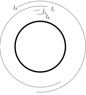
Proof. Let us fix a positive integerN satisfying the condition of the proposition (see Figure 1). The operators H := N1L0 + 24c (N − N1)1, L+ := N1L−N and L− := N1LN satisfy the following relations on Dfin:
[H, L±] = ∓L±, [L−, L+] = 2H, L± =L∗∓.
Moreover H is diagonalizable with non-negative eigenvalues only, the span of its eigenvec- tors is exactly Dfin which is an invariant core for the operators L±. It then follows that these operators generate a strongly continuous, positive energy unitary representation of the universal coverM¨obg of the Möbius group. This construction — both at the Lie algebra as well as the Lie group level — was already considered and used by various authors; see e.g. the work [34]. In particular,
P = 1
4(2H−L+−L−) and P˜= 1
4(2H+L++L−)
Id Ic
Ik
I˜k
Figure 1: Intervals Ic, Id covering S1 and Ik,I˜k with N = 36.
are conjugate to each other by the unitary operator eiπH, with P being the self-adjoint generator of “translations” with spectrum Sp(P) = Sp( ˜P) = R+∪ {0}. Moreover, by [4, Theorem 3.3] we have the relation
e−2sH =e−tanh(s2)Pe−sinh(s) ˜Pe−tanh(s2)P (3) for alls >0. Let us now consider howP andP˜can be written in terms of the stress-energy T. We have
P = 1
4n(2L0−L−N −LN) + c 48
N − 1 N
1=T(p) +b1 and likewise P˜=T(˜p) +b1, where
b= c 48
N − 1 N
and p and p˜ are the functions defined by the formulas p(z) = 4n1 (2− zN −z−N) and
˜
p(z) = 4N1 (2 +zN +z−N).
The function pis nonnegative onS1 and it has exactly N points where its value is zero:
p(z) = 0 ⇐⇒ z =ei2πNk fork = 1, . . . N.
All these null-points are of course local (and also global) minima, where the derivative is zero. We can thus “cut” pintoN “nice” pieces: p=p1+. . .+pN where the support of the nonnegative function pk is the closure of the arc
Ik =
eiθ : k−1 N < θ
2π < k N
,
and kpkk32 < ∞. This latter follows from the fact that pk is once differentiable and its derivative is of bounded variations; see the similar considerations at [9, Lemma 5.3]. Thus for every k = 1, . . . N,
Pk =T(pk) + b N1
is a well-defined self-adjoint operator affiliated toAU(Ik) and we have P =P1+. . .+PN. Since the terms in this decomposition are affiliated to commuting factors, just as in the proof [39, Proposition 3.2], we have that
Sp(P1) +. . .+ Sp(PN) = Sp(P) = R+∪ {0}.
On the other hand, the spectrum of the operatorsPk(k = 1, . . . N)must all coincide, since using rotations one can easily show that they are all unitary conjugate to each other. It then follows that each of them must be a positive operator. Thus for the bounded operator e−tanh(s2)P appearing in formula (3), we have the local decomposition into a product of commuting bounded operators
e−tanh(s2)P = YN
k=1
e−tanh(s2)Pk where the norm of each term is smaller or equal than 1.
Let us turn to P˜. As we have P˜ = AdeiNπL0(P), the localization of P˜k =AdeiNπL0(Pk) are different from that of P: P˜k is affiliated toAU( ˜Ik)whereI˜k =eiNπIk andAU is defined in Section 2 (we are considering the intervals as subsets in C). With this localization, we can still assure the strong commutation between Pk and P˜j whenever k 6= j, j + 1 (mod N). So in the decomposition
e−2sH = e−tanh(s2)P e−sinh(s) ˜P e−tanh(s2)P
=
YN
k=1
e−tanh(s2)Pk
! N Y
k=1
e−sinh(s) ˜Pk
! N Y
k=1
e−tanh(s2) ˜Pk
!
we can make some rearrangements. Note that e−2sH = r−L0r2q, where q = 48c (N2 −1) if we set r = e−2s/N. To shorten notations, let us introduce the self-adjoint contractions Xk=e−tanh(s2)Pk and Yk =e−sinh(s) ˜Pk. For simplicity, we did not indicate their dependence on r, but note that in the range 0 < r < 1 they depend norm-continuously on r (for t >0, x≥0, the function e−tx is uniformly continuous in t).
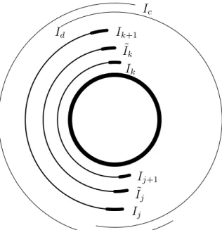
All X-operators and separately, all Y-operators commute between themselves, and moreover [Xl, Ym] = 0 whenever l 6=m, m+ 1(modN). Recall that 6πN is smaller than the length of each of the intervals ofIc∩Id. Therefore, by cyclically renaming the intervals (but keeping the relation betweenIkandI˜kand the corresponding localization of the operators), we may assume that there are1≤k < j≤N such thatIk∪Ik+1 andIj∪Ij+1 are included in the different connected components of Ic ∩Id. Furthermore, to fix the notation, we
Ic
Id
Ik I˜k
Ik+1
Ij+1
I˜j Ij
Figure 2: Localization of the factors of Cr. The indicated intervals I•,I˜• correspond to thick segments. The operatorsQj+1
l=kXl,Qj
l=kYl, Qj
l=k+1Xl are localized in the arcs, from the inside, respectively. The corresponding factors inDr are localized in the complements of these arcs, respectively.
may assume that Ik∪ · · · ∪Ij+1 ⊂ Ic, while Ij ∪ · · · ∪IN ∪I1· · · ∪Ik ⊂ Id. Note that I˜k∪ · · · ∪I˜j ⊂Ic and I˜j ∪ · · · ∪IN ∪I1· · · ∪I˜k−1 ⊂Id (see Figure 2).
By the localization explained above, we obtain r−L0r2q =
YN
l=1
Xl
! N Y
l=1
Yl
! N Y
l=1
Xl
!
=
k−1Y
l=1
Xl
j+1Y
l=k
Xl YN
l=j+2
Xl
! k−1 Y
l=1
Yl Yj
l=k
Yl YN
l=j+1
Yl
! k Y
l=1
Xl Yj
l=k+1
Xl YN
l=j+1
Xl
!
=
j+1Y
l=k
Xl
Yj
l=k
Yl
Yj
l=k+1
Xl
! k−1 Y
l=1
Xl
YN
l=j+2
Xl k−1Y
l=1
Yl
YN
l=j+1
Yl
Yk
l=1
Xl
YN
l=j+1
Xl
! . (4)
Here the first part Cr = Qj+1 l=kXlQj
l=kYlQj
l=k+1Xl
is an element of AU(Ic), where whereas the second part Dr = Qk−1
l=1 XlQN
l=j+2XlQk−1 l=1 YlQN
l=j+1YlQk
l=1XlQN l=j+1Xl
is an element of AU(Id).
By construction, kCrk,kDrk ≤ 1. Thus, we have obtained the desired decomposition r−L0 = (r1qCr)(r1qDr).
In the above proposition we specifically worked with L0. However, by considering the adjoint actions ofU(γ)for all diffeomorphisms γ ∈Diff+(S1)on the decompositions found above, it is now easy to draw the following conclusion.
Corollary 3.2. Let Ic, Id ∈ I be two open proper arcs such that Ic ∪Id = S1, and f a strictly positive smooth function on S1. Then there exist two norm-continuous families of operators (0,1)∋r7→Cr ∈ AU(Ic) and(0,1)∋r 7→Dr ∈ AU(Id) such that rT(f) =CrDr.
4 Further decompositions
In this section, we shall consider further decompositions of rL0, for which the crucial ingredient will be a result of Neretin [36]. Though in his work the relevant theorem is stated for representations which are direct sums of those highest weight ones, as was already mentioned, a positive energy, strongly continuous, projective unitary representation of Diff+(S1) can only be of that form. For better readability, we shall recall the statement that we are going to exploit. We will need the concept ofanalytic diffeomorphism; we will denote by Diff+a(S1) the set of γ ∈ Diff+(S1) that extends to an annulus around S1 ⊂ C in a complex analytic manner.
Theorem 4.1. [36, Theorem 2] Let U be a positive energy, strongly continuous, projec- tive unitary representation of Diff+(S1) with the associated conformal Hamiltonian L0. Then elements of the form U(γ)rL0U(˜γ) (r ∈ (0,1], γ,˜γ ∈ Diff+a(S1)) form a projec- tive semigroup: for any γ1, γ2,γ˜1,γ˜2 ∈ Diff+a(S1) and r1, r2 ∈ (0,1] there exist some γ3,γ˜3 ∈Diff+a(S1)), r3 ∈(0,1] such that
U(γ1)r1L0U(˜γ1)
U(γ2)r2L0U(˜γ2)
=U(γ3)r3L0U(˜γ3), where of course equality is meant in the projective sense.
Actually, what we shall really use is a certain adaptation of the above result for the case oftrue(and not just projective) representations of the Möbius group. Note that every Möbius transformation is of course analytic. To make the necessary modifications, we shall first make an observation2.
Lemma 4.2. Let(A, U,Ω) be a conformal net. ThenU(γ)Ω∈CΩif and only ifγ ∈M¨ob.
Proof. We need to show the “only if” part; the other direction is true by definition. If γ = id, the statement immediately follows, otherwise, by composing a Möbius element g, we may assume that γ fixes three points onS1. Let I1, I2, I3 be three intervals with such end points.
2Roberto Longo suggested another idea for the proof of Lemma 4.2: as in the proof in the main text, we may assume that γ preserves three points. As U(γ) preserves the vacuum vector, it commutes with the modular group of the three intervals between these points, hence with the whole Möbius group. From this it is straightforward thatγ= id.
By contradiction, let us assume that γ 6= id. Then there is a point s ∈ S1 such that γ(s) 6= s. As γ fixes three points on S1, it also preserves each interval bounded by any pair of these points. Say limnγn(s) =: s∞ (for a single element γ ∈Diff+(S1), S1 can be decomposed into intervals such that γ is monotone on each interval, hence such a limit exists).
It is not restrictive to assume that I1, the closure of I1, contains neither {γn(s)} nor s∞. Let us go to the real line picture (which is only necessary below, in order to simplify the conformal distance) and call I1 := (t1, t2), and I := (s, s∞) (or (s∞, s) depending on in which direction s is moved, without losing the generality, we may assume the former case). Assume that I1 andI are bounded intervals on the line. Now they are separated by a finite distance.
We can pick x ∈ A(I1) and y ∈ A(I) such that hxΩ, yΩi 6= 0 by Reeh-Schlieder property. We may further assume that hΩ, xΩi = 0 = hΩ, yΩi, as we can subtract their vacuum expectation. By the assumption that U(γ)Ω ∈ CΩ and [18, Conformal cluster theorem], we obtain
|hxΩ, yΩi|=|hx(U(γ)∗)nΩ, y(U(γ)∗)nΩi|
=|hAdU(γ)n(x)Ω,AdU(γ)n(y)Ωi|
≤ (t2−t1)(s∞−γn(s))
(γn(s)−t1)(s∞−t2)kxkkyk →0,
as γn(s)→ s∞, while other distances remain finite. This is a contradiction, hence γ = id under the assumption that γ fixes three points.
Corollary 4.3. Let V be a strongly continuous, unitary representation of M¨ob with pos- itive energy, with the associated conformal Hamiltonian L0. Then elements of the form V(γ)rL0V(˜γ) consist a semigroup: for any g1, g2,g˜1,˜g2 ∈ M¨ob and r1, r2 ∈ (0,1], there exist some g3,g˜3∈M¨ob, r3 ∈(0,1) such that
V(g1)r1L0V(˜g1)
V(g2)rL20V(˜g2)
=V(g3)r3L0V(˜g3) in the proper (not only projective) sense.
Proof. Consider the well-known conformal net usually referred as the U(1)-current net [5]. One may restrict its projective unitary representation U of Diff+(S1) to the Möbius group and arrange its phase factors in such a way that the vacuum Ωwill be an invariant vector (see Section 2). In this way we get a positive energy, strongly continuous, unitary representation V of M¨ob in which all such irreducible representations (i.e. every possible integer highest weight) appear: this is evident because for every n ≥ 1, the dimension of (n+ 1)th energy space is strictly larger than the dimension of the nth one. Thus, if we can show the statement for our particular representation V, we have proved it for all positive energy representations ofM¨ob. By applying Theorem 4.1 toU of theU(1)-current
net, we obtain that for every g1, g2,g˜1,˜g2 ∈ M¨ob and r1, r2 ∈ (0,1] there must exist some γ3,γ˜3 ∈Diff+a(S1) and an r3 ∈(0,1] such that
U(g1)r1L0U(˜g1)
U(g2)rL20U(˜g2)
=U(γ3)r3L0U(˜γ3)
in the projective sense. If r1 = r2 = 1, then of course g3 and g˜3 can be chosen to be in M¨ob. On the other hand, ifr1r2 <1, then they must be inM¨ob. Indeed, in such a case r must be strictly smaller than1(the right hand side cannot be unitary as the left hand side does decrease the length of some vectors). Then “sandwiching” the left hand sides byΩ— i.e. considering the scalar product hΩ,·Ωi for the left hand side (which is of course only defined up-to-phase) — gives a complex number of modulus1, whereas by Lemma 4.2 and the fact CΩ is the unique eigenvector of L0 with the eigenvalue 0, the same sandwiching of the right hand side gives a number of modulus 1 if and only ifγ3,γ˜3 ∈M¨ob.
Considering the relevant unitary operators rather than projective ones, we therefore have that for everyg1, g2,g˜1,g˜2 ∈M¨obandr1, r2 ∈(0,1]there must exist someg3,˜g3 ∈M¨ob and an r3 ∈ (0,1] such that V(γ1)r1L0V(˜γ1)
V(γ2)r2L0V(˜γ2)
and V(γ3)rL30V(˜γ3) are proportional to each other. The proof is then finished by evaluating both sides on Ω and concluding that this proportion must be 1.
Corollary 4.4. Let V be a positive energy, strongly continuous, unitary representation of M¨ob with associated conformal Hamiltonian L0. There exists some r, r1, r2 ∈ (0,1) and g, g1, g2 ∈M¨ob, g 6= id, such that
rL0 =rH11r2H2V(g) in the proper sense, where Hj =AdU(gk)(L0) (k = 1,2).
Proof. We choose two elementsg˜1,˜g2 ∈M¨obsuch thatH˜k =AdV(˜gk)(L0), andH˜1 andH˜2
do not strongly commute: such choices are actually abundant, sinceL0 is maximally abelian in the Lie algebra. Then there must exist somer1, r2 ∈(0,1)such that rH1˜1 andr2H˜2 do not commute (otherwise their generators would strongly commute by analytic continuation).
Now we apply Corollary 4.3 to r1H˜1r2H˜2 = V(˜g1)r1L0V(˜g1)∗V(˜g2)r2L0V(˜g2)∗ to obtain g3,g˜3 ∈M¨oband r ∈(0,1) such that
V(˜g1)rL10V(˜g1)∗V(˜g2)r2L0V(˜g2)∗ =V(g3)rL0V(˜g3)∗, in the proper sense, or equivalently,
rL0 =V(g3−1g˜1)rL10V(g3−1˜g1)∗V(g−13 g˜2)r2L0V(g3−1˜g2)∗V(g3˜g3).
By defininggk =g3−1˜gk, hence accordinglyHk :=AdV(g3−1g˜k)(L0)andg :=g3g˜3, we obtain the desired equality. To check that g 6= id, note that by our choice of H˜k, r1H1 and r2H2 do not commute as well. Yet, in the equality
rL0 =r1H1r2H2V(g),
the left-hand side is self-adjoint, while if g = id, the right-hand side would not be self- adjoint. Therefore, g 6= id.
Proposition 4.5. Let A be a conformal net, U be the associated projective unitary rep- resentation of Diff+(S1), and L0 the conformal Hamiltonian. For some r ∈ (0,1), there exists a Möbius transformationg 6= id, such that for anyIc, Id∈ I be two open proper arcs such that Ic∪Id =S1 we have two bounded operators C ∈ AU(Ic) and D ∈ AU(Id) such that we have the decomposition
rL0 =CDU(g) in the proper sense.
Proof. We apply Corollary 4.4 to obtainr, r1, r2 ∈(0,1),g ∈M¨ob, g6= id and H1, H2 such that
rL0 =r1H1r2H2U(g).
Then we apply Corollary 3.2 toHk with the intervalsKk,c, Kk,d such thatKk,c ⊂Ic, Kk,d ⊂ Id and K1,d∩K2,c =∅ (see Figure 3), to obtain operators Ck, Dk such that rkHk =CkDk. By the localization, C2 and D1 commute.
Hence it holds that rL0 =rH11r2H2U(g) =C1D1C2D2U(g) =C1C2D1D2U(g), and C :=
C1C2 is localized in K1,c∪K2,c ⊂ Ic, while D:=D1D2 is localized in K1,d∪K2,d ⊂ Id, as desired.
Id
Ic
K1,c K1,d
K2,c K2,d
Figure 3: Intervals Ic, Id, K1,c, K1,d, K2,c, K2,d.
5 Normality of the product vacuum state
We can now prove our main claim: for a conformal net on S1 — where by “conformal”
we mean that it has the full diffeomorphism covariance (see Section 2) — the split property is automatic. Let (A, U,Ω)be a conformal net, and assume Ia, Ib ∈ I are two open proper arcs separated by a positive distance.
Consider the ∗-algebra A(Ia)∨algA(Ib) generated by the commuting factors A(Ia)and A(Ib). We shall now introduce a family {φz} of functionals on this algebra indexed by a complex number z, |z| ≤1. For a generic element X ∈ A(Ia)∨algA(Ib),
X = Xn
k=1
AkBk (n ∈N, Ak ∈ A(Ia), Bk ∈ A(Ib)) (5) and a complex number z in the closed unit disk D1 ={z ∈C:|z| <1}, let
φz(X) = Xn
k=1
hΩ, AkzL0BkΩi.
The above quantity is well-defined in the sense that it indeed depends only on z and X, but not on the particular decomposition chosen for X. Indeed, since A(Ia) and A(Ib) are commuting factors, there is a natural isomorphism between the algebraic tensor product A(Ia)⊙A(Ib)andA(Ia)∨algA(Ib), see [38, Proposition IV.4.20]. In particular, the bilinear formA(Ia)× A(Ib)∋(A, B)7→ hΩ, AzL0BΩi ∈C extends to a unique linear functionalφz
onA(Ia)∨algA(Ib).
Note that the expressionzL0 is indeed a well-defined bounded operator for every z ∈ D1
(for z = 0, we define it by continuity in the strong operator topology, hence to be the projection P0 onto CΩ): this is because Sp(L0) ⊂ N. That is, we are using not just the positivity ofL0, but also that elements of its spectrum are all integers (e.g.z12 =√
z would be ambiguous).
For everyX ∈ A(I1)∨algA(I3), the mapz 7→φz(X)is analytic in D1. In fact, denoting by Pm the spectral projection of L0 associated to the eigenvalue m, we have the power series decomposition of φz(X)
φz(X) = Xn
k=1
X∞
m=0
hΩ, AkPmBkΩizm.
Since P0 =hΩ, · iΩis the one-dimensional projection on the vacuum vector, we have that φ0(X) =
Xn
k=1
ω(Ak)ω(Bk),
i.e. φ0 is the product vacuum state, whereas φ1 = ω. Thus, in view of Proposition 2.2, in order to prove the split property, we need to show that while “changing” the parameter
z from 1 to 0, the functional φz remains normal. In particular, it would be desirable to obtain estimates onkφ1−φ0k.
The idea of considering φz not only at the pointsz = 1 andz = 0, but on a larger area (so that its analytic dependence onz can be exploited) comes from [18]. There the authors work with the function z 7→ φz(AB) to obtain a bound on |φ1(AB)−φ0(AB)| for a pair of elements A ∈ A(I1) and B ∈ A(Ib) thereby proving the conformal cluster theorem for a Möbius covariant net. However, their estimate involves the product of norms kAk kBk; when it is reformulated for an element X of the considered form (5), we get some bounds in terms of P
kkAkk kBkk, rather than in terms of the norm of X. Hence their method does not give a useful estimate on kφ1−φ0k. In fact, they cannot obtain anything that would imply the split property: this is because they only use Möbius covariance, and as was mentioned in the introduction, counterexamples to the split property exist when diffeomorphism covariance is not assumed [9, Section 6].
Instead, our idea is the following: using diffeomorphism covariance and in particular the decompositions of rL0 established in the previous sections, we can show that φz depends norm-continuously on z and is normal (i.e. extends to a normal linear functional of the von Neumann algebra A(Ia)∨ A(Ib)) when z is in a certain region. Unfortunately, the region directly obtainable by such decompositions do not contain the desired point z = 0.
However, if this region contains a ring encircling the pointz = 0 (and as we shall see, this will exactly be the case) we can use general complex analytic arguments (essentially the Cauchy theorem) to deduce normality of φ0:
Lemma 5.1. Let r0 ∈ (0,1) be a fixed radius and suppose that φz is normal whenever
|z|=r0 and that on the circle with radius r0, r0S1 ∋z 7→φz is norm-continuous. Then φ0
is also normal.
Proof. We shall use some well-known technical facts. In particular, we shall exploit that the norm-limit of a sequence of normal functionals on a von Neumann algebraMis normal (see e.g. [27, Corollary 7.1.13]). To apply this fact, one should note that the norm is defined on the von Neumann algebra M, but by the Kaplansky density theorem, the norm of a normal functional onA(Ia)∨A(Ib)is equal to the norm of its restriction toA(Ia)∨algA(Ib).
Therefore, in the following we do not distinguish them.
Thus one has — e.g. by considering Riemann-sums — that ifϕ : [s1, s2]∋t7→ϕt∈ M∗ is a norm-continuous family of normal linear functionals, then ϕ(·) = Rs2
s1 ϕt(·)dt is also a well-defined normal functional onM.
Since D1 ∋z 7→φz(X) is analytic, by the Cauchy integral formula we have φ0(X) = 1
2πi I
r0S1
φr0eiθ(X) dz z for every X ∈ A(Ia)∨algA(Ib).
Let us now discuss how the decompositions rL0 help us out in different regions of D1. LetIc =Ia′, andIdbe an (open) interval containing the closure ofIabut not intersectingIb.