3.1 Construction of the iteration

Variable preconditioning for strongly nonlinear elliptic problems

by B. Borsos¹, J. Kar´atson² Abstract

Variable preconditioning has earlier been developed as a realization of quasi-Newton methods for elliptic problems with uniformly bounded nonlinearities. This paper presents a generalization of this approach to strongly nonlinear problems, first on an operator level, then for elliptic problems allowing power order growth of nonlinearities. Numerical tests reinforce the convergence results.

Key words. Variable preconditioning, quasi-Newton methods, iterative methods, nonlinear elliptic problems

AMS subject classifications. 65N30, 47N20.

1 Introduction

Nonlinear elliptic problems arise in various applications for models that describe stationary states. We may mention, for instance, elastoplasticity, magnetic potential equations, and flow problems in physics and other fields, see, e.g., [4, 6, 7, 10] and the references there. As shown by such works as well, a widespread way to solve such problems is to use finite element discretization (FEM) and then to apply a Newton-like iteration, see also [1, 5, 11]. A general approach to construct quasi-Newton methods has been given in [9], where approximate Jacobians are defined via spectral equivalence, and hence they can be regarded as variable preconditioners.

This method, as well as much of the mentioned theory, is applicable to problems with uniformly bounded nonlinearities that allow well-posedness in the underlying Hilbert function space.

The goal of this paper is to extend the above approach of variable preconditioning to prob- lems with stronger nonlinearities without a uniform boundedness assumption. This situation covers power order growth of nonlinearities, which also appears in various physical models. First we generalize the Hilbert space method of [9] to a class of unbounded nonlinearities in Section 2. Then the result is applied to a class of elliptic problems with power order nonlinearities in Section 3. Numerical tests reinforce the theoretical convergence results.

2 Variable preconditioning for strongly nonlinear oper- ator equations

LetH be a real Hilbert space with inner product h., .iand corresponding norm k · k. We study operator equations

F(u) = 0

1Department of Analysis, Technical University; Budapest, Hungary

2Department of Applied Analysis & MTA-ELTE Numerical Analysis and Large Networks Research Group, ELTE University; Department of Analysis, Technical University; Budapest, Hungary

for a given nonlinear operator F : H → H. Our goal is to extend Theorem 3.1 in [9] to nonlinearities without a uniform boundedness assumption, and thereby to prove the convergence of a proper iteration with variable preconditioning.

The allowed strong nonlinearity of the operator means that both the upper spectral bounds and the Lipschitz constants of the Gˆateaux derivatives are allowed to grow up to infinity along with the norms of the arguments. The setting is based on [9, Section 3], however, its technique has to be essentially redone to follow and eliminate the effect of the non-uniform nonlinearities.

This is done in such a way that the variable bounds are incorporated in a modified recursive estimation of the residuals. Thus one can ensure that the overall convergence is not spoiled by the growth of nonlinearities. The method and its convergence are formulated as follows.

Theorem 2.1. Let H be a real Hilbert space and F :H →H a nonlinear operator. LetF have a Gˆateaux derivative that satisfies the following properties:

(i) For any u∈H the operator F⁰(u) is self-adjoint.

(ii) There exists a constant λ >0 and a continuous increasing function Λ : R⁺→R⁺ such that the following condition is satisfied:

λkhk² ≤ hF⁰(u)h, hi ≤Λ(kuk)khk² (∀u, h∈H). (2.1) (iii) There exists a continuous increasing function L:R⁺→R⁺ satisfying

kF⁰(u)−F⁰(v)k ≤L(max{kuk, kvk})ku−vk (∀u, h∈H). (2.2) Denote by u^∗ ∈ H the unique solution of F(u) = 0. Let M ≥ m > 0 be given constants, and for any n∈N let us choose a bounded self-adjoint linear operator B_n :H →H such that

mhB_nh, hi ≤ hF⁰(u_n)h, hi ≤MhB_nh, hi (∀h∈H). (2.3) Then the sequence, defined by

u_n+1 :=u_n− 2

M +mB_n⁻¹F(u_n) (∀n ∈N), (2.4) converges locally linearly to u^∗, namely, there exists a neighbourhood U of u^∗ and for given u0 ∈U there exists a constant C >0 such that

ku_n−u^∗k ≤C

M −m M +m

n

(∀n ∈N). (2.5)

The proof will be preceded by suitable lemmas. First, for a given bounded self-adjoint strictly positive operatorA, the following notation stands for the energy inner product: hu, viA:=

hAu, vi, and the corresponding norm isk · k_A. The following properties are known for spectrally equivalent operators:

Lemma 2.1. [9] Let A and B be bounded self-adjoint linear operators on H with positive lower bound, and let there exist constants M ≥m >0 such that

mhBh, hi ≤ hAh, hi ≤MhBh, hi (∀h∈H). (2.6)

Then

mhA⁻¹h, hi ≤ hB⁻¹h, hi ≤MhA⁻¹h, hi (∀h∈H) (2.7)

and

I− 2

M +mAB⁻¹ A⁻¹

≤ M−m

M +m. (2.8)

Lemma 2.2. The preconditioning operators in (2.3) have uniformly bounded inverses, namely,

kB_n⁻¹k ≤λ⁻¹M (∀n∈N). (2.9)

Proof. The upper and lower estimates in (2.3) and (2.1), respectively, yield:

λkhk² ≤ hF⁰(u_n)h, hi ≤MhB_nh, hi ≤MkB_nhkkhk (∀h∈H). (2.10) Dividing by λkhk and using that B_n :H →H is bijection, we obtain the desired bound.

Remark 2.1. The main assumption in the theorem is the local Lipschitz continuity of F⁰, so we will derive some of its consequences below. In fact, it is easy to see that (2.2) implies the upper bound in (2.1): for any u, h∈H

hF⁰(u)h, hi=h(F⁰(u)−F⁰(0))h, hi+hF⁰(0)h, hi ≤ L(kuk)kuk+kF⁰(0)k khk²,

i.e. we have a bound of the form Λ(kuk)khk² with the real function Λ(t) := L(t)t+kF⁰(0)k.

This upper assumption in the theorem is only present in order to indicate the analogy with the cited earlier result.

Notations. In what follows, the functions Λ andLwill be often evaluated on balls, in particular when we follow the iteration steps fromu_n tou_n+1. Hence the following notations will be used:

let

Λ˜∗ := Λ(ku^∗k), (2.11)

and for fixedn ∈N let

L˜_n,n+1 :=L(max{ku_nk,ku_n+1k}), L˜_n,∗ :=L(max{ku_nk,ku_∗k}). (2.12) Furthermore, we introduce the following energy norms:

khk_u :=hF⁰(u)⁻¹h, hi^1/2 (for givenu∈H), k · k_∗ :=k · k_u^∗, k · k_n:=k · k_un (2.13) (for given n ∈ N). It follows readily (with Lemma 2.1) that for fixed u the norms k · k_u and k · k are equivalent, namely:

λ^1/2khk_u ≤ khk ≤Λ^1/2(kuk)khk_u (∀h ∈H). (2.14) Two important special cases are

khkn ≤λ^−1/2khk, khk ≤Λ˜^1/2_∗ khk∗ (∀h∈H). (2.15) The norms k · k∗ and k · k_n are related by the following non-uniform extension of [9, Cor. 3.4]:

Lemma 2.3. For all h∈H we have 1

1 +µ_n(u_n) ≤ khk²_∗

khk²_n ≤1 +µ_n(u_n), (2.16) where

µ_n(u_n) := ˜Ln,∗Λ˜^1/2_∗ λ⁻²kF(u_n)k∗ . (2.17) Proof. The lower bound in (2.1) implies a corresponding lower estimate for the variation of F:

kF(u)−F(v)k ≥λku−vk (∀u, v ∈H). (2.18) This, together with the assumptions (2.1)–(2.2) on F⁰, implies

hF⁰(u)h, hi ≤ hF⁰(v)h, hi(1+L(max{kuk, kvk})λ⁻²kF(u)−F(v)k) (∀u, v, h∈H). (2.19) For the case u=u^∗ and v =u_n, this gives hF⁰(u^∗)h, hi ≤ hF⁰(u_n)h, hi(1 + ˜Ln,∗λ⁻²kF(u_n)k).

Using (2.15) and reversing the role of u^∗ and un, we obtain 1

1 +µ_n(u_n) ≤ hF⁰(u^∗)h, hi

hF⁰(u_n)h, hi ≤1 +µ_n(u_n) (∀h∈H). (2.20) From this, Lemma 2.1 yields the desired estimate.

Proof of Theorem 2.1. The proof is carried out in several steps.

(1) The existence and uniqueness of the solution u^∗ ∈H is well-known for such potential prob- lems, see, e.g., [6]. The major part of the proof will be the derivation of the local convergence of the residuals, i.e. lim_n→∞kF(u_n)k= 0. Then (2.18) will yield that lim_n→∞u_n =u^∗ as well.

(2) The proof can be started in a similar way as in [9], but even in this first part we must follow more carefully the non-uniform constants. For given n ∈Nin the iteration,

F(u_n+1) =F(u_n) +F⁰(u_n)(u_n+1−u_n) +R(u_n). (2.21) In this situation, analogously to inequalities (18)–(19) in [9], one can estimate the linear part (from Lemma 2.1) and the remainder as follows, using that (owing to (2.1)) F⁰ is Lipschitz continuous in the ball B(0,max{ku_nk,ku_n+1k}) with a corresponding constant ˜L_n,n+1:

kF(u_n) +F⁰(u_n)(u_n+1−u_n)k_n ≤ M−m

M +mkF(u_n)k_n, (2.22) kR(u_n)k_n ≤ 2 ˜L_n,n+1

λ^1/2(M +m)²kB_n⁻¹F(u_n)k². (2.23) Here a further estimation can be given: using that (2.9) and (2.15) yield

kB_n⁻¹F(u_n)k ≤λ⁻¹MkF(u_n)k ≤λ⁻¹MΛ˜^1/2_∗ kF(u_n)k∗ (2.24) and letting K := _λ5/2^2M_(M^2Λ_+m)^˜∗ ₂, (2.23) implies

kR(u_n)k_n ≤KL˜_n,n+1kF(u_n)k²_∗, (2.25)

Let us estimate the k · k_n-norm of F(u_n+1) in (2.21), using (2.22) and (2.25):

kF(u_n+1)k_n≤ M −m

M +mkF(u_n)k_n+KL˜_n,n+1kF(u_n)k²_∗, (2.26) hence Lemma 2.3 yields

kF(u_n+1)k∗ ≤(1 +µ_n(u_n))^1/2

M −m

M +m(1 +µ_n(u_n))^1/2+KL˜_n,n+1kF(u_n)k∗

kF(u_n)k∗. (2.27) (3) We formulate a recurrence for the sequence kF(u_n)k_∗ as follows. By definitionµ_n(u_n)≥0, thus (1 +µ_n(u_n))^1/2 ≥1, consequently

kF(u_n+1)k∗ ≤(1 +µ_n(u_n))

M −m

M +m +KL˜_n,n+1kF(u_n)k∗

kF(u_n)k∗. (2.28) By substituting the definition (2.17) of µ_n(u_n) and defining the real function

ϕ_n(t) := (1 + ˜Ln,∗Λ˜^1/2_∗ λ⁻²t)

Q+KL˜_n,n+1t

, where Q:= M −m

M +m, (2.29) the estimate (2.28) can be reformulated as

kF(u_n+1)k∗ ≤ϕ_n(kF(u_n)k∗)kF(u_n)k∗. (2.30) However, this recurrence cannot be directly used to derive convergence, since ϕn is a stepwise varying function containing ˜L_n,n+1 and ˜L_n,∗. Below we will show that these constants can be estimated as a function of kF(u_n)k∗, so that finally ϕ_n can be estimated independently of n.

(4) For the estimation of the constant ˜L_n,n+1we need to bound max{ku_nk,ku_n+1k}in terms of kF(u_n)k∗ and fixed constants. Here the definition (2.4) yields

kun+1k ≤ kunk+ 2

M +mkB_n⁻¹F(un)k (∀u∈[un, un+1]), (2.31) hence a bound for max{ku_nk,ku_n+1k} can be obtained as a bound for the above r.h.s. Here, first, (2.18) yields kF(u_n)−F(0)k ≥λku_nk, hence, also using (2.15),

ku_nk ≤λ⁻¹ kF(u_n)k+kF(0)k

≤λ⁻¹ Λ^1/2_∗ kF(u_n)k_∗+kF(0)k

. (2.32)

Further, to estimate kB_n⁻¹F(u_n)k, we use Lemma 2.2 and (2.15) to derive for all h ∈ H that kB_n⁻¹hk ≤λ⁻¹MΛ˜^1/2∗ khk∗ , hence

kB_n⁻¹F(u_n)k ≤λ⁻¹MΛ˜^1/2_∗ kF(u_n)k∗. (2.33) Thus, summing up, we have

max{ku_nk,ku_n+1k} ≤λ⁻¹Λ˜^1/2_∗ 1 + 2M M +m

kF(u_n)k∗+λ⁻¹kF(0)k =: f(kF(u_n)k∗),

where the real function f :R⁺0 →R⁺0 is defined as f(t) :=λ⁻¹Λ˜^1/2_∗ 1 + 2M

M +m

t +λ⁻¹kF(0)k. (2.34)

Hence the estimation of the constant ˜L_n,n+1 can be given as

L˜_n,n+1 :=L(max{ku_nk,ku_n+1k})≤L_f(kF(u_n)k∗), (2.35) where

L_f(t) := L(f(t))

is an increasing continuous function (since bothLand f have this property), andL_f is already independent of n.

(5) Similarly, for the estimation of the constant ˜Ln,∗ we need to bound max{kunk,ku^∗k}in terms of kF(u_n)k_∗ and fixed constants. Now, using (2.18),

ku^∗k ≤λ⁻¹kF(0)k,

further, kunk has the larger bound (2.32), hence the latter is also a bound for their maximum:

max{ku_nk,ku^∗k} ≤λ⁻¹ Λ^1/2_∗ kF(u_n)k∗ +kF(0)k .

Hence

L˜_n,∗ :=L(max{ku_nk,ku_∗k})≤L_g(kF(u_n)k_∗) (2.36) using the increasing continuous functions

g(t) :=λ⁻¹Λ˜^1/2_∗ t+λ⁻¹kF(0)k, L_g(t) :=L(g(t)). (2.37) (6) Altogether, using (2.35) and (2.36), the function (2.29) can be estimated as

ϕ_n(t)≤(1 +L_g(t) ˜Λ^1/2_∗ λ⁻²t) (Q+KL_f(t)t) =: ϕ(t), (2.38) and accordingly, inequalities (2.30) and (2.38) result in

kF(u_n+1)k∗ ≤ϕ(kF(u_n)k∗)kF(u_n)k∗, (2.39) where ϕis an increasing continuous real function and is independent of n.

(7) Now it can be shown, just as in [9], that if the initial guess satisfies

ϕ(kF(u₀)k∗)<1, (2.40)

then limn→∞kF(u_n)k∗ = 0. In fact, using notation r:=ϕ(kF(u₀)k∗), estimate (2.39) and the monotonicity of ϕ, one can derive by induction that

kF(u_n)k∗ ≤rⁿkF(u₀)k∗ →0 (asn → ∞). (2.41) Here (2.15) implies lim

n→∞kF(u_n)k= 0 in the original norm too, and then, as mentioned in item

(1) of the proof, (2.18) yields that limn→∞u_n=u^∗ as well.

(8) It remains to show the estimate (2.5), which means that the convergence factor can be improved to

Q:= M−m M +m

independently of u₀. The main point is to derive this rate for the weigthed residual errors

en :=kF(un)k∗, (2.42)

First observe that the continuity of ϕand e_n →0 imply

n→∞lim ϕ(e_n) = ϕ(0) =Q. (2.43) Further, by (2.39), the errors satisfy

e_n≤

n−1

Y

k=0

ϕ(e_k)

! e₀ =

n−1

Y

k=0

ϕ(ek) Q

!

Qⁿe₀ (∀n ∈N). (2.44) For all k we have e_k ≤e₀, thus we have L_g(e_k)≤L_g(e₀), L_f(e_k)≤L_f(e₀) (∀k ∈N). Using (2.38) and introducing the notations d₁ := ˜Λ^1/2∗ λ⁻²L_g(e₀), d₂ :=KL_f(e₀), we obtain

ϕ(e_k)≤(1 +d₁e_k) (Q+d₂e_k). (2.45) This and (2.41) imply

ϕ(ek)

Q ≤(1 +d₁e_k) (1 +d₃e_k) = 1 +d₄e_k+d₅e²_k ≤1 +d₄e₀r^k+d₅e²₀r^2k, (2.46) with constants d₃ = ^d_Q², d₄ =d₁+d₃, d₅ =d₁d₃. From here we can follow [9] to deduce the following upper estimate from (2.44):

e_n≤exp

d₄e₀

1−r + d₅e²₀ 1−r²

e₀Qⁿ ≡Ee₀Qⁿ. (2.47) This, together with (2.15) and (2.18), yields

kun−u^∗k ≤λ⁻¹kF(un)k ≤λ⁻¹Λ˜^1/2_∗ kF(un)k∗ =:λ⁻¹Λ˜^1/2_∗ en ≤λ⁻¹Λ˜^1/2_∗ e0EQⁿ, (2.48) hence (with constantC :=λ⁻¹Λ˜^1/2∗ e₀E) we obtain (2.5).

3 Application to power order nonlinear elliptic problems

In this section we apply the obtained iterative method to the finite element discretization of a strongly nonlinear elliptic problem with power order nonlinearity. Let Ω ⊂ R^N be a bounded domain, let p≥ 3 and k₁, k₂ >0 be given constants, g ∈L²(Ω) a given function, and consider

the following boundary value problem:

( −div (k1+k2|∇u|^p−2) ∇u

= g,

u|∂Ω = 0, (3.1)

Such a nonlinear operator, which is of regularized p-Laplacian type, arises, e.g., in electrorhe- ological fluid models, where p = 4, see [2]. Problem (3.1) has a unique weak solution in the Sobolev space W₀^1,p(Ω), see, e.g., [13].

We apply the finite element method (FEM) for the discretization of the problem. Let V_h be a given FE subpace of certain continuous piecewise polynomial functions, then we look for u∈V_h such that

Z

Ω

(k1+k2|∇u|^p−2)∇u· ∇v = Z

Ω

gv (∀v ∈Vh). (3.2)

Our goal is to define the corresponding iterative method for this problem and to prove its convergence.

3.1 Construction of the iteration

First we cast the problem into the setting of section 2. Our Hilbert space H will be the finite dimensional space V_h, endowed with the H₀¹ Sobolev inner product and induced norm

hu, vi:=

Z

Ω

∇u· ∇v, kuk_H¹

0 :=k∇uk_L², (3.3)

respectively. Note that, owing to p > 2, we have V_h ⊂ W₀^1,p(Ω) ⊂ H₀¹(Ω), further (since V_h is finite dimensional), k∇uk_L^p and k∇uk_L² define equivalent norms on V_h, in particular, there exists a constant ˆc >0 such that

k∇uk_L^p ≤cˆk∇uk_L² (∀u∈V_h). (3.4) This shows that although the original BVP is posed in the Banach space W₀^1,p(Ω), the Hilbert space structure on V_h is a proper choice.

The operator F :Vh →Vh, corresponding to our problem, is defined in a weak form as hF(u), vi ≡

Z

Ω

(k₁+k₂|∇u|^p−2)∇u· ∇v− Z

Ω

gv (∀u, v ∈V_h). (3.5) Then the FEM problem (3.2) is equivalent to findingu∈V_h such thathF(u), vi= 0 (∀v ∈V_h), or simply

F(u) = 0 inV_h.

We want to apply the iteration, defined in Theorem 2.1, with properly chosen operatorsB_nthat approximate the Gˆateaux derivativesF⁰(u_n). For this, we first have to determine the operators F⁰(u_n). Here (3.5) can be written as

hF(u), vi= Z

Ω

f(∇u)· ∇v− Z

Ω

gv, (3.6)

using the notationf : R^N →R^N defined by

f(η) := (k₁+k₂|η|^p−2)η (η ∈R^N). (3.7) The derivative of f at someη ∈R^N is the Jacobian matrix

∂ηf(η) = k2(p−2)|η|^p−4(η·η^T) + (k1+k2|η|^p−2)I, (3.8) whereη·η^T denotes the diadic matrix with entries η_iη_j (i, j = 1, ..., N). Following [3, 6], the Gˆateaux derivativeF⁰(u) satisfies

hF⁰(u)h, vi= Z

Ω

∂_ηf(∇u)∇h· ∇v, (3.9)

which means that the diffusion coefficient in the operator F⁰(u_n) is the full matrix∂_ηf(∇u).

In order to significantly simplify this operator, one can propose to omit the diadic matrices, and to include only the second term in (3.8) to obtain an operator with diagonal diffusion coefficient. Therefore we introduce the operators B_n : V_h →V_h defined by the following weak forms: for given un∈Vh in the iteration, let

hB_nh, vi ≡ Z

Ω

k₁+k₂|∇u_n|^p−2

∇h· ∇v (∀h, v ∈V_h). (3.10) Then we obtain the following sequence from (2.4). Let u₀ ∈ V_h be given and assume that u_n∈V_h is constructed. Then u_n+1 is found as follows:

( solve Bnzn=F(un);

let u_n+1 :=u_n− _M+m² z_n. (3.11)

In particular, the auxiliary equation B_nz_n=F(u_n) can be written in weak form as hB_nz_n, vi=hF(u_n), vi (∀v ∈V_h).

That is, introducing the linear functional

`_nv :=hF(u_n), vi ≡ Z

Ω

(k₁+k₂|∇u_n|^p−2)∇u_n· ∇v− Z

Ω

gv (v ∈V_h), the update z_n ∈V_h is the solution of the linear elliptic FEM problem

Z

Ω

k₁+k₂|∇u_n|^p−2

∇z_n· ∇v =`_nv (v ∈V_h). (3.12)

3.2 Convergence of the iteration

Proposition 3.1. The nonlinear operator F, defined by (3.5), and the linear operators Bn, defined by (3.10), satisfy the conditions of Theorem 2.1.

Proof.

(1) The Jacobians (3.8) are symmetric, hence (3.9) is self-adjoint. First we check that F

satisfies (2.1) and (2.2). As mentioned in Remark 2.1, the upper bound in (2.1) can be omitted, since it follows from (2.2). The lower bound is straightforward withλ:=k1, namely, (3.8) and (3.9) with v =h yield

hF⁰(u)h, hi= Z

Ω

k2(p−2)|∇u|^p−4(∇u· ∇h)²+ Z

Ω

(k1+k2|∇u|^p−2)|∇h|² ≥k1khk²_H1

0. (3.13) Now we have to prove the local Lipschitz property (2.2) in H₀¹-norm. Since the Gˆateaux derivatives of F are symmetric for all u∈H₀¹, therefore F⁰(u)−F⁰(v) is also symmetric, thus its operator norm can be calculated using its quadratic form:

kF⁰(u)−F⁰(v)k= sup

khkH1 0=1

|h(F⁰(u)−F⁰(v))h, hi|= sup

khkH1 0=1

Z

Ω

(∂ηf(∇u)−∂ηf(∇v))∇h· ∇h .

(3.14) To estimate the integrand, we first study the norms of the tensors ^∂2_∂η^f(η)2 , which satisfy

∂²f(η)

∂η²

= sup

|h|=1

∂²f(η)

∂η² (h, h, h)

(3.15) owing to their symmetry [12]. Such tensors are discussed in [8] including general nonlinearities of the following form:

f(η) =a(|η|²)η, (3.16)

where r 7→ a(r) is a smooth scalar function. Using the notations a⁰_r(r), a⁰⁰_r(r) for the first two derivatives ofa, the formula in [8] for (3.16) implies

∂²f(η)

∂η² (h, h, h) = 6a⁰_r(|η|²)(η·h)|h|²+ 4a⁰⁰_r(|η|²)(η·h)³.

In our case, (3.7) is defined by the scalar nonlinearity a(r) :=k₁+k₂r^p−22 , for which we have a⁰_r(r) =k₂ p−2

2 r^p−42 , a⁰⁰_r(r) =k₂ (p−2)(p−4) 4 r^p−62 . Substitution and Cauchy-Schwarz inequalities yield

∂²f(η)

∂η² (h, h, h) = 3k2(p−2)|η|^p−4(η·h)|h|²+k2(p−2)(p−4)|η|^p−6(η·h)³,

∂²f(η)

∂η² (h, h, h)

≤k₂(p−2)(3 +|p−4|)|η|^p−3|h|³ =: c₂(p)|η|^p−3|h|³, where c₂(p) :=k₂(p−2)(3 +|p−4|). Hence (3.15) gives

∂²f(η)

∂η²

≤c₂(p) sup

|h|=1

|η|^p−3|h|³ =c₂(p)|η|^p−3. (3.17) Now, with the application of the mean value theorem on the derivative function ∂_ηf in an

arbitrary segment [η₁, η₂], we get k∂_ηf(η₁)−∂_ηf(η₂)k ≤ sup

η∈[η˜ 1, η2]

∂²f

∂η²(˜η)

· |η₁−η₂| ≤c₂(p) max{|η₁|^p−3,|η₂|^p−3}|η₁−η₂|.

(3.18) Combining this with (3.14), we obtain

kF⁰(u)−F⁰(v)k ≤ sup

khk_H1 0=1

Z

Ω

k∂_ηf(∇u)−∂_ηf(∇v)k |∇h|² (3.19)

≤c₂(p) sup

khkH1 0=1

Z

Ω

max{|∇u|^p−3,|∇v|^p−3}|∇u− ∇vk∇h|² ≤

≤c2(p) sup

khk_H1 0=1

Z

Ω

|∇u|^p−3|∇u− ∇v||∇h|²+ Z

Ω

|∇v|^p−3|∇u− ∇v||∇h|²

.

(3.20)

In this expression we can apply H¨older’s inequality of the following four-term form:

Z

Ω

|f|^p−3|g₁g₂g₃| ≤ kfk^p−3_Lp kg₁k_L^pkg₂k_L^pkg₃k_L^p (∀f, g₁, g₂, g₃ ∈L^p(Ω)), (3.21) which yields

kF⁰(u)−F⁰(v)k ≤c₂(p) k∇uk^p−3_Lp +k∇vk^p−3_Lp

k∇u− ∇vk_L^p sup

khkH1 0=1

k∇hk²_Lp.

(3.22) Owing to (3.4), we can apply the estimate k∇zkL^p ≤cˆkzk_H¹

0 in each norm above, thus we get kF⁰(u)−F⁰(v)k ≤c₂(p) ˆc^p

kuk^p−3_H1 0

+kvk^p−3_H1 0

ku−vk_H¹

0 sup

khk=1

khk²_H1

0 ≤

≤2c₂(p) ˆc^p

max{kuk_H¹

0,kvk_H¹

0}^p−3

ku−vk_H¹

0,

(3.23)

hence F⁰ is locally Lipschitz continuous with the Lipschitz coefficient function L:R⁺0 →R⁺0: kF⁰(u)−F⁰(v)k ≤L(max{kuk_H¹

0,kvk_H¹

0})ku−vk_H¹

0, L(t) =c_pt^p−3 (3.24) where cp := 2c2(p) ˆc^p.

(2) We prove that the operator B_n in (3.10) satisfies (2.3) with proper uniform constants M and m. Lower estimation of (3.13) gives

hF⁰(u_n)h, hi ≥ Z

Ω

k₁ +k₂|∇u_n|^p−2

|∇h|² =hB_nh, hi, (3.25)

and upper estimation of (3.13) with Cauchy-Schwarz inequality yields hF⁰(u_n)h, hi ≤

Z

Ω

k₂(p−2)|∇u_n|^p−4|∇u_n|²|∇h|²+ Z

Ω

(k₁+k₂|∇u_n|^p−2)|∇h|²

= Z

Ω

(k1+k2(p−1)|∇un|^p−2)|∇h|² ≤(p−1) Z

Ω

(k1+k2|∇un|^p−2)|∇h|² = (p−1)hBnh, hi. (3.26) Hence (2.3) holds with lower and upper bounds

m:= 1, M :=p−1.

Now we can readily formulate

Theorem 3.1. The iteration (3.11), defined in Subsection 3.1, converges locally according to the estimate

ku_n−u^∗k_H¹

0 ≤C

1− 2 p

n

(∀n ∈N). (3.27)

Proof. By Proposition 3.1, the conditions of Theorem 2.1 are satisfied, further, iteration (2.4) coincides with (3.11) in our situation. Hence (2.5) holds locally, and for the obtained bounds m= 1 and M =p−1 the convergence factor is

M−m

M +m = 1− 2

p. (3.28)

Remark 3.1. Alternatively to (3.10), the preconditioner may be defined with a different con- stant ˜k₂ >0 instead of k₂:

hB_nz, vi:=

Z

Ω

k₁+ ˜k₂|∇u_n|^p−2

∇z· ∇v, (3.29)

in order to try to balance between k₁ and k₂. A simple calculation shows that the modified bounds then become m = min

1, ^k_˜²

k₂ , M = max 1, ^k_˜²

k₂(p−1) . Then it is easy to see that the estimation of the convergence factor cannot be improved in this way: that is, if k₂ ≤k˜₂ ≤ k₂(p−1) then we recover ^M−m_M+m = 1− ²_p just as in Theorem 3.1, whereas for values of ˜k₂ outside the interval [k₂, k₂(p−1)] we even obtain larger convergence factors. One may expect to make a reasonable choice by either defining the constant to be in the middle of the interval [k₂, k₂(p−1)] (that is, ˜k₂ :=k₂ ^p₂ as a formal balance between the two endpoints) or leaving ˜k₂ :=k₂. Both choices ensure convergence with the speed as in Theorem 3.1.

Remark 3.2. The obtained result provides linear convergence. Based on the techniques of [9], it can be expected that one may obtain convergence of higher order up to 2 if a sharper approximation of the derivatives is available. This and other extensions are the subject of forthcoming research.

3.3 Numerical experiments

Consider the following boundary value problem:

( −div (χ₁+χ₂|∇u|²)∇u

= g,

u|∂Ω = 0, (3.30)

whereχ₁, χ₂ >0 are given constants. Such a nonlinear operator arises, e.g., in electrorheological fluid models, see [2]. This problem, which describes a stationary fluid, is a special case of (3.1) with p = 4. Our test domain is the unit square Ω := [0,1]², and we use piecewise linear finite elements.

We apply the iteration (3.11) with preconditioning operators (3.29):

hB_nh, vi ≡ Z

Ω

χ₁+ ˜χ₂|∇u_n|²

∇h· ∇v (∀h, v ∈V_h). (3.31) Since p= 4, here we letχ₂ ≤χ˜₂ ≤3χ₂ as suggested in Remark 3.1, and we obtain from (3.28) that the theoretical convergence factor is

M −m M+m = 1

2 independently of the constants χ₁, χ₂.

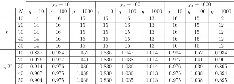
We have run the iteration (3.11)–(3.12) with the following variation of parameters. A uniform mesh was used with N = 10,20, . . . ,50 node points in each direction. Since the equation can be scaled, we letχ1 = 1 and we variedχ2 using the values 10,100,1000. Similarly, we defined g as a constant with values 10,100,1000. The initial guess u₀ was the solution of the Poisson equation with r.h.s. g. We measured the relative residual error

ε_n := kF(u_n)k_H¹

0

kF(u₀)k_H¹

0

throughout the iteration.

The results with the choice ˜χ₂ := χ₂ are given in Table 1. The upper part contains the number n of iterations to achieve accuracy εn < 10⁻⁶. The lower part contains the values of ε_n2ⁿ, i.e. the ratio of ε_n with the expected relative residual error 1/2ⁿ. (We have repeated the tests with ˜χ₂ := 2χ₂, then we obtained very similar but slightly worse results.)

We may observe that the actual convergence follows very closely the expected theoretical error. Further, both the number of iterations and the relative residual errors behave in a robust way w.r.t. the variation of all parameters.

χ₂ = 10 χ₂ = 100 χ₂ = 1000

N g = 10 g = 100 g = 1000 g = 10 g = 100 g = 1000 g = 10 g = 100 g = 1000

n

10 14 16 15 15 16 13 16 15 12

20 14 16 15 15 16 13 16 15 12

30 14 16 15 15 15 13 16 15 12

40 14 16 15 15 15 13 16 15 12

50 14 16 15 15 15 13 16 15 12

ε_n2ⁿ

10 0.837 0.984 1.052 0.835 1.047 1.014 0.984 1.052 0.934

20 0.926 0.977 1.041 0.830 1.038 1.014 0.977 1.041 0.901

30 0.914 0.976 1.039 0.830 1.036 1.014 0.976 1.039 0.895

40 0.907 0.975 1.038 0.830 1.036 1.013 0.975 1.038 0.894

50 0.904 0.975 1.038 0.830 1.035 1.013 0.975 1.038 0.895

Table 1: Number of iterations to achieve ε_n <10⁻⁶ and ratio with the expected relative residual error.

3.4 Conclusions

We have generalized the variable preconditioning quasi-Newton approach to strongly nonlinear elliptic problems and derived its convergence. Numerical tests reinforce the theoretical results, moreover, the method exhibits robust convergence w.r.t. the variation of the coefficients and the mesh size.

Acknowledgement. This research was supported by the Hungarian Scientific Research Fund OTKA, No. K112157 and SNN125119.

References

[1] Axelsson, O. and Maubach, J., On the updating and assembly of the Hessian matrix in finite element methods, Comput. Methods Appl. Mech. Engrg., 71 (1988), pp. 41–67.

[2] Busuioc, V., Cioranescu, D., On a class of electrorheological fluids. Contributions in honor of the memory of Ennio De Giorgi, Ricerche Mat.49 (2000), suppl., 29–60.

[3] Ciarlet, Ph., The finite element method for elliptic problems, North-Holland, Amster- dam, 1978

[4] Ciarlet, Ph., Linear and nonlinear functional analysis with applications,SIAM, Philadel- phia, 2013.

[5] Deuflhard, P. and Weiser, M., Global inexact Newton multilevel FEM for nonlinear elliptic problems, in Multigrid Methods V, Lect. Notes Comput. Sci. Eng. 3, Springer, Berlin, 1998, pp. 71–89.

[6] Farag´o I., Kar´atson J., Numerical Solution of Nonlinear Elliptic Problems via Precon- ditioning Operators: Theory and Application.Advances in Computation, Volume 11, NOVA Science Publishers, New York, 2002.

[7] Glowinski, R.,Variational Methods for the Numerical Solution of Nonlinear Elliptic Prob- lems, SIAM, Philadelphia, 2015.

[8] Kar´atson J. , On the Lipschitz continuity of derivatives for some scalar nonlinearities, J. Math. Anal. Appl. 346 (2008) 170-176.

[9] Kar´atson J., Farag´o I., Variable preconditioning via quasi-Newton methods for non- linear problems in Hilbert space, SIAM J. Numer. Anal., Vol. 41, No. 4, pp. 1242-1262, 2003.

[10] Kˇriˇzek, M. and Neittaanm¨aki, P. , Mathematical and Numerical Modeling in Elec- trical Engineering: Theory and Applications, Kluwer Academic Publishers, Dordrecht, The Netherlands, 1996.

[11] Rossi, T., Toivanen, J., Parallel fictitious domain method for a non-linear elliptic Neumann boundary value problem, Numer. Linear Algebra Appl. 6 (1999), no. 1, 51–60.

[12] Waterhouse, W. C.,The absolute-value estimate for symmetric multilinear forms,Lin- ear Algebra Appl. 128 (1990), 97–105.

[13] Zeidler, E., Nonlinear functional analysis and its applications, Springer, 1986