Introduction of Flexible Production Bids and Com- bined Package-Price Bids in a Framework of In- tegrated Power-Reserve Market Coupling
D´avid Csercsik
P´azm´any P´eter Catholic University
Faculty of Information Technology and Bionics, H-1083 Budapest, Pr´ater u. 50/A csercsik@itk.ppke.hu
Abstract: In this article a multi-zonal integrated energy-reserve market model is proposed.
Bidders in this model may submit their demand and supply bids on the one hand in the form of conventional hourly step bids and block bids, which are cleared and paid according to market clearing prices (MCPs). On the other hand, suppliers may submit so called flexible production bids, while both suppliers and consumers may submit fill-or-kill type package- priced combined bids – these bids are accepted if their acceptance implies an improvement in the resulting total social welfare, which the market clearing algorithm aims to optimize.
The model includes network constraints for the nominal case (if no reserves are activated) and also for perturbed cases when the allocated reserves are activated.
Keywords: Integrated markets; Co-optimization; Market coupling; Market design
1 Introduction
The most important aim of European-type day-ahead electricity markets is to har- monize power demand and supply in a way, which in ideal case results in the highest possible social welfare (SW). The concept of SW basically originates from the ’pay as clear’ principle [1]. In the most simple framework for electricity market clearing, supply and demand bids are submitted for a single period of the trading interval, each bid being described by two parameters, the bid quantity and the bid price per unit (PPU). In the case of demand bids, the product of the bid quantity and the PPU describes the willingness to pay for the required quantity, while in the case of supply bids, the same product corresponds to the minimal required income for the offered amount (usually assumed to be equal to the cost of the production). The market is cleared according to the so calledmarket clearing price(MCP): Demand bids with bid PPU lower than the MCP will be rejected, as well as supply bids with bid PPU higher than the MCP. Bids whose PPU is equal to the MCP may be also partially accepted.
Bids are paid for according to the MCP, which means that the bidder, e.g. in the case of an accepted demand bid, pays less for the required quantity compared to his willingness to pay (and similarly, supply bidders receive potentially more payment for accepted supply bids). This surplus, which is the product of the difference be- tween the bid PPU and the MCP and the bid quantity, is called the social welfare (SW) of the bid [1]. The total social welfare (TSW) of a dispatch is the sum of SW values corresponding to single bids, and may be represented as the area between the supply and the demand curve as depicted in Fig. 1.
Figure 1
Social welfare of single bids in the one-period market model. Siand Dicorrespond to supply and demand bids, while MCP stands for the market clearing price.
In the simple one-period example depicted in Fig. 1, the maximization of TSW is trivial: The MCP is determined from the intersection of supply and demand curves (this will ensure the energy balance), and clear the market according to this MCP. In general case however, nonconvexities originating from special bid types (see later )make the problem complex. On the other hand, multiple price zones connected with transmission lines may be present. In this case the energy balance is not required for every single price zone, but it must hold for the total system, while the transmission constraints of the connecting lines must be taken into account [2].
In addition, operators of the power system have to ensure the stability and security.
In the current setup, it is assumed that the central authority operates the market with regard to the transmission system as well - in line with this, the terminology of independent system operator (ISO) is used throughout the paper.
Stability refers to frequency stability [3] or voltage stability [4], while security refers to e.g. n-1 line and node contingency, which means that if one of the lines or one of the nodes of the network fails instantly, the resulting flows may not overload any of the remaining lines [5]. The stability of frequency is dependent on the supply- demand balance: If consumers or suppliers deviate from their predefined schedule, and thus cause imbalance, the ISO activates previously allocated (positive or nega- tive) reserves at generating units to restore the balance.
These reserves practically mean rights for the ISO to give orders to generating units to increase or decrease actual generation values. In most of the countries where a liberalized electricity trade takes place, separate markets were created for the allo- cation of such and other reserves, called altogether ancillary services [6].
Joint (or integrated) energy and reserve markets are representing a concept, where the allocation of power and reserve to generating units takes place not on disjoint markets, but in one integrated auction [7].
One main benefit of integrated markets is described in [8] as: ’co-optimization en- ables the participants to achieve more surplus by providing an efficient way to sub- mit all possible combinations of energy-reserve allocation to the market. There- fore the risk of precommitting generating capacity to sequential offers of different products and clearing can be eliminated’. The paper [9] formulates a similar con- sideration as ’Since distinct reserve services can in fact be strongly coupled, and the heuristics required to bridge the various sequential markets can ultimately lead to loss of social welfare, simultaneous energy/reserves market-clearing procedures have been proposed and are in use. However, they generally schedule reserve ser- vices subject to exogenous rules and parameters that do not relate to actual operat- ing conditions’.
The paper [9] proposes a security constrained simultaneous clearing of energy and reserve services with a perturbation approach similar to the one proposed in the cur- rent paper. The supply side in [9] is also formulated in a unit-commitment spirit.
The approach of the paper [10] is similar, it also proposes that at any given network bus all scheduled reserve types should be priced not at separate rates but at a com- mon rate equal to the marginal cost of security at that bus. The papers [11, 12] use a multiobjective mathematical programming (MMP) approach including MCPs as well in the formulation.
While several results have been already published in the field of integrated markets, the presented approaches usually are driven by the unit-commitment spirit of North American market models, where the generating units are not self-scheduling. A not self-scheduling clearing means that generating units submit technical characteristics and production costs to the ISO who determines production profiles and reserve allocations according to these parameters.
In European type markets, the self-scheduling generating units may bid with a va- riety of products, and act like more active market participants [13]. An approach for co-optimizing power and reserve allocation which is motivated by this type of power market is described in the articles [8, 14, 15].
The main aim of the current paper is to provide a possible framework for multi- node integrated markets, but in contrast to the cost minimization approach used e.g.
in [16], the proposed concept aims to maximize the total social welfare (SW).
In the day-ahead market, where the clearing is determined for 24 consecutive hours, technological considerations of generating units imply further challenges (in inte- grated and conventional markets as well). Startup costs and minimal operating loads are the most common sources of non-convexities, but also minimal up and down
times can be considered. These non-convexities are usually handled by the intro- duction of block orders, which may be rejected or accepted in a binary manner (no partial acceptance is allowed), thus the representative variables in the clearing are binary.
An approach to represent the constant and variable costs (corresponding to start-up and production respectively) of generating units is the concept of minimum income condition (MIC) orders [17–20]. As described in [19], ’minimum income orders are supply orders consisting of several hourly step bids for potentially different market hours, and they are bound together by the MIC which prescribes that the overall income of the MIC order must cover its given costs’. The efficient clearing of such bids is described in [20]. In this framework, generation costs corresponding to this type of bid are zero if the bid is rejected, otherwise they are considered with a fixed and a linear variable term which are determined by the bidder. Incomes in the case of the proposed MIC bid can be expressed as the product of accepted quantities and MCPs. In this concept, since the elements of the MIC bids are standard hourly step bids, the generation profile of the unit submitting the MIC bid is fully determined by the MCPs.
In this paper a somewhat different approach is proposed, namely the concept of flexible production bids(shortly FP bids) and combined bids is introduced. Flexible production bids are formed in the spirit of unit commitment: The production values for the single periods are determined by the ISO during the clearing, considering the technical and cost parameters of the unit. Technical parameters are the load gradient constraints, while the cost parameters are the start-up and variable cost values. Combined bids in contrast hold fixed quantities of power and reserve and are cleared and paid as a whole package if accepted.
In addition, the coupling of combined power-reserve markets is also considered, which means that transmission constraints are formulated on nominal flows and also on flows originating from the activation of reserves are.
The proposed framework may be also considered as a kind of transition between European and US type markets in the sense that on the one hand conventional price- quantity (step) bids are submitted, and on the other hand generating units may also submit generation characteristics in the form of FP bids, in which case their power and reserve allocation will be scheduled by the ISO. In addition, participants may also submit fixed-price combined bids, which represent basically pay-as-bid type bids.
Since the problem formulation in itself is a complex challenge (even if one considers only ’conventional’ coupling of integrated markets without innovative bid types), this paper presents only the important concepts of the formulation.
2 The Market Model
The basis of the proposed framework is a standard uniform price (European type) multi-node (or in other words zonal) electricity market model withT time periods
(see e.g. the basic structure in [1]).
In the current paper only reserves corresponding to frequency control (more pre- cisely secondary reserves) are considered. It is assumed that reserve-providing units are paid for the allocation of reserve capacities, in other words in the current model it is not taken into account if reserves are activated or not.
2.1 Bid Types in the Model
We suppose in the following that one period of the model corresponds to one hour.
2.1.1 One Hour Bids
One-hour single-product bids These bids are the principal elements of the mar- ket model. They describe demand or supply of a single product (power, positive or negative reserve) in a single time period, and their acceptance is independent of the acceptance of bids regarding other time periods.
It can be assumed that most bids are submitted in this format to the market. These bids are characterized by a quantity (B), by the index of the time period in which the bid is relevant (t) and a respective price (per unit), denoted byΘ.
Such one-hour bids are cleared according to MCPs denoted byϕiP(t),ϕiRp(t)and ϕiRn(t)corresponding to power, positive and negative reserve respectively in each nodei, regarding the respective time periodt. If the resulting MCP is equal PPU of a bid, the partial acceptance of the bid is allowed, formally the bid acceptance indicatoryis∈[0,1]in this case.
2.1.2 Multiple Period Bids
Multiple period bids may include more than one periods as well, but must be taken into account and cleared as a single bid.
Block bids In the used terminology, block bids refer to a single product (power or reserve) bids, which includes multiple (consecutive) time periods. It is assumed that block bids have the fill-or-kill property, in the sense that either the total of- fered quantity is either fully accepted for all respective time periods, or the bid is completely rejected.
These bids are characterized by quantities for the corresponding hours (B– a vector in this case), by the indices of the time periods in which the bid is relevant (t) and the respective PPUs, denoted by Θ(also a vector). Although in the practice the bid quantities and PPUs usually are the same for every period of the bid, the vector formulation allows potentially different quantities and PPUs for each period.
The acceptance constraint in the case of block bids is that the resulting total SW must be positive [21]. The total SW of a block bid is the sum of the SWs corresponding
to the included time periods. Block bids are very common in electricity markets and they are discussed e.g. in [21, 22].
Remark: Standard bids In the used terminology, standard bids mean to 1-hour single-product bids or block bids. As the acceptance of such bids is explicitly deter- mined by MCPs, they are distinguished from the bid types described in the follow- ing,
Flexible production bids Flexible production or FP bids are suited for generat- ing units who practically offer their generating capacity in a unit-commitment type offer. Upon the acceptance of such bids, the ISO assigns nonzero power and reserve amounts to units submitting these bids for each period included in the bid, accord- ing to the actual needs of the market. These bids are characterized in the proposed model by start-up cost (α), variable cost (β) and ramp constraints (RUfor ramp-up andRDfor ramp-down). The maximal possible amount of assigned reserve is deter- mined by the assigned power production profile and by the ramp constraints (e.g. if in two consecutive periods the output of the unit according to the power production profile is increased withRU, no positive reserve may be assigned to it).
If an FP bid is accepted, the generating unit is paid off according to produced quan- tities (determined by the ISO) and respective MCPs, and its income must cover the reported expenses of generation, derived from start-up and variable costs. The for- mulation of last consideration may be viewed as a variant of the so called minimum income condition (MIC) [18, 19, 23].
Example 1 In the following, the concept of FP bids is demonstrated using a sim- ple 2 period example. The set of standard (in this case only 1-hour) bids is as summarized in Table 1.
Table 1
Standard bids in of example 1 (the upper index in the bid ID refers to the period)
bid ID relevant period quantity (B) PPU (Θ)
D11 1 15 90
D12 1 20 80
S11 1 27 75
S12 1 13 85
D21 2 15 90
D22 2 20 80
S21 2 27 75
S22 2 13 85
It can be seen in Table 1 that the standard bids are the same for hour 1 and 2, thus they imply the supply-demand curves depicted in Fig. 2 for both hours.
Figure 2
Supply-demand curves of example 1
First, one may consider the scenario where no other bids are present. In this case, the dispatch calculation is very simple: The MCP (denoted byϕ) is determined by the intersection of the curves (ϕ=80): D1 andS1will be fully accepted whileD2 will be partially accepted. The social welfare of the demand and supply side in each period may be calculated as:
SWD= (90−80)15=150 SWS= (80−75)27=135
thus the total social welfare equals to 285 for each period thusT SW=570.
On the other hand, one can assume a scenario, when in addition to the standard bids, an FP bid is also present with the parametersα=3000,β=28 (we can assume that RUandRDare arbitrary positive values).
What happens, if ϕ=72 for both periods? According to the MCP, the standard supply bids will be rejected (as their PPU is higher than the MCP), while both demand bids will be fully accepted, resulting in the social welfare
SWD= (90−72)15+ (80−72)20=430
for both periods. Regarding the supply side, the unit corresponding to the FP bid has to produce 35 MW in each period. The cost of the production of the FP bid may be calculated asα+2β35=4960, while the income of the FP bid is 35·72·2=5040.
The income of the bid covers the production cost (which is a necessary condition for the acceptance of the FP bid), andSWS=80. In this caseT SW =860+80=940.
As theT SW is higher in the case of the second scenario (940 vs 570), if the FP bid is also present in the market, the market clearing algorithm will prefer the second solution, as it aims to maximize the T SW. In general, in order to maximize the TSW, the market clearing algorithm has to determine the MCPs and the acceptance of FP bids simultaneously.
It can be noted furthermore that the acceptance of the FP bid is not explicitly de- termined by the MCP: If the PPU of the first and the second supply bid is lowered to 60 and 72 respectively, and supposeϕ=72, both demand bids will be accepted (whileS2will be partially accepted to ensure the power balance) and this results in
SWD= (90−72)15+ (80−72)20=430 SWS= (72−60)27=324
for each period, resulting inT SW =1508, a solution clearly preferable compared to the acceptance of the FP bid.
Regarding the notations corresponding to FP bids in the model, multiple nodes are considered in general, it is assumed that each FP bid corresponds to a generating unit in a certain node of the network. Each node may hold multiple generating units, but not all nodes necessarily hold generating units. Binary variables are used to describe whether a generating unit operates or not in a given time period. vi j(t)denotes the activity indicator of unit j of nodeiat timet. Units are indexed from 1 in each node. For example if there are 2 units in node 1 and 1 unit in node two, variables v11(t),v12(t)andv21(t)will represent the activity indicators for each time periodt.
With the help of these binary variables, start-up costs, minimal up and down times and minimal load of units can be described. On the other hand, if the corresponding activity indicator is 0, the output of the unit is 0 (regarding power, and both types of reserves as well). Pi j(t)denotes the power production value allocated to unit j of nodeiat timet. Regarding reserves,Rpi j(t)andRni j(t)denote respectively the positive and negative reserve value allocated to unit jof nodeiat timet.
Combined bids Combined bids in the proposed framework make possible to sub- mit bids simultaneously for power and reserve production (or consumption). In the case of combined bids, the bid holds fixed values of power, positive and negative re- serves, potentially including multiple time periods. The parameters of this bid type are the amounts of products offered for the respective time periods, and total price.
The price is not interpreted as per unit in this case, but as a total amount, which shall be at least paid to the bidder upon acceptance – independent of MCPs. In addition to this fixed price, to each combined bid a nonnegative surplus is assigned by the MO (see the details later).
it is assumed that combined bids have the fill-or-kill property and the standard bids and combined bids are calledfixed quantity(FQ) bids (in contrast to FP bids where the quantity is assigned to the bid by the ISO).
Example 2 A single-period scenario is used to illustrate the concept of combined bids, where the standard power and reserve bids are as summarized in table 2 (the power bids define the same supply-demand curves as in Example 1). In the case of this simple example only one type of reserve is considered (arbitrarily + or -).
Again, it is assumed that no other bids are present. In this case ϕP=80,ϕR= 45, resulting inSWP=285 andSWR=50 (T SW =335) – the balance is 27 MW regarding power and 10 MW regarding the reserve.
bid ID quantity (B) PPU (Θ)
DP1 15 90
DP2 20 80
SP1 27 75
SP2 13 85
DR1 10 50
DR2 10 40
SR1 15 45
Table 2
Standard bids in of example 2 (the upper index refers to power/reserve)
On the other hand, if in addition to the standard bids, also assume a combined bid offering 15 MW of power and 15 MW of reserve at the price of 1600 is present, the following dispatch is possible. Regarding the power balance, ifϕP=75, both demand bids are accepted resulting in the demand of 35 MW, from which 20 MW of power is supplied from the first standard supply bid (which is partially accepted), and the rest from the combined bid.
Regarding the reserve balance, the standard reserve supply bid is rejected, the first standard reserve demand bid is fully accepted while the second one is partially ac- cepted. All 15 MWs of reserve are supplied by the accepted combined bid.
Here, two conditions must be checked. First, the total income from demand bids must cover the total cost of supply. The income from power demand bids is(15+ 20)75=2625, while the income from reserve demand bids is(10+5)40=600, thus the total income is 3225. The cost of the standard power supply bid is 75·20=1500, while the cost of the combined bid is 1600 The total cost is 3100 – the difference between the total income and the total cost (125) will be assigned to the surplus of the combined bid in this case.
Second, theT SW must exceed theT SW of the first scenario in order to make the dispatch more desirable for the clearing algorithm.
SWP= (90−75)15+ (80−75)20=325 SWR= (50−40)10=100 ,
while the SW of the combined bid is equal to its surplus (125), thusT SW=540>
335.
2.1.3 Overview of Bids
Fixed quantity and flexible production For all bids (except for FP bids) it may be calculated how much they will contribute to power and reserve balances upon their acceptance (partial acceptance is allowed only in the case of one-hour single- product bids). Thus,these bids are called fixed quantity (FQ) bids. In the proposed model demand bids are always FQ. The setBcollets all FQ bid types, regarding
the traded product (not distinguishing between one-hour and multiple hour bids).
B={DP, SP, DRp,SRp, DRn, SRn, DC,SC} (1) The first letter stands for demand or supply, while the rest stand for power (P), pos- itive reserve (Rp), negative reserve (Rn) or combined bids (C). These abbreviations are used through the paper.
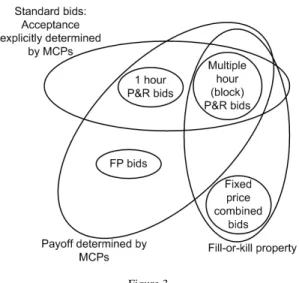
Figure 3 summarizes the bid types used through the paper and their properties.
Figure 3
Bid types in the proposed market formulation. P&R stands for power and reserve.
2.2 Clearing of the Market
One may depict the one-hour single product (e.g. power) demand and supply bids for any particular hour in the standard spot-market fashion like in Fig. 4. By such an ordering of bids (increasing by PPU in the case of supply and decreasing in the case of demand), if there are enough bids for the curves to intersect in every hour, setting the MCPs according to the intersection prices clears the market (in this case however no block bids, FP bids or combined bids are taken into account, thus all of such bids are rejected).
On the other hand if the MCP is as depicted in Fig. 4, it can be seen that there is an imbalance both in the supplied/consumed power (Bd1−Bs1), and regarding incomes/costs as well. The total income isI1+I2=Bd1ϕwhile the total cost of the accepted supply bid isC1=Bs1ϕ. To put the principle of the clearing very short, the excess income (summed for all hours) is used to pay for block, FP and combined bids which cover the hourly power/reserve imbalances (as detailed in Example 1 of subsection 2.1.2 and depicted in Fig. 2)
The task of the market-clearing algorithm is to find such MCPs, and such scheduling of FP, block and combined bids (via determination of their scheduling/acceptance
Figure 4
Power and income/cost imbalances caused by the particular depicted MCP.ϕstands for the MCP, while θdandθsdenotes the demand and supply bid prices.
variables1), which maximizes the total social welfare, and respects the hourly power and reserve balance constraints as well as the network bottlenecks.
3 Formalization of the Market Clearing Model
In the current article, the main ideas and the most important corresponding equations of the proposed concepts are presented. The detailed mathematical formalism of the optimization problem describing market clearing can be found in the freely available research report [24] available atarxiv.org/pdf/2004.13466.pdf.
Nnodes are assumed in the network. The number of units at nodeiis denoted byni, and it is assumed that each unit submits a FP bid. The total number of units, which do submit FP bids is denoted byn.mTi denotes the number of bids of type T at node i. T ∈ {DP,SP,DRp,SRp,DRn,SRn,DC,SC}, where the first letter corresponds to Demand/supply, and the further letters correspond to power (P), positive (Rp) or negative (Rn) reserve or combined bids (C). Furthermore,mT =∑imTi.
3.1 Model variables
3.1.1 Variables Corresponding to the Clearing of FP Bids
vi j(t) denotes the up indicator of unit j of nodei at timet, equals to 1 if unit j of nodeiis operating at time periodT and zero otherwise. The vector of all such variables is denoted byv∈ {0,1}n(T+1). vi j(O)is an auxiliary variable, which is
1 To be more precise, in the case of combined bids, the payoff variables have to be deter- mined as well
equal to one if the unit is up in any of the periods in the analyzed time frame (used for the calculation of start-up costs). The structure ofvis detailed in [24].
Pi j(t)denotes the power production value allocated to unit j of nodeiat timet, Rpi j(t)denotes the positive reserve allocated to unitjof nodeiat timet, andRni j(t) denotes the negative reserve allocated to unit j of nodeiat timet. P∈ {0,1}nT, Rp∈ {0,1}nT,Rn∈ {0,1}nT. The structure of the vectorsP,RpandRnis detailed in [24].
3.1.2 Variables Corresponding to MCPs and Bid Acceptance Indicators ϕiT(t) T ∈ {P, Rp, Rn} denotes the MCP of power / positive reserve /negative reserve at nodeiat timet.ybi jis the bid acceptance indicator of the standard bid of typeb∈B(see eq. 1), corresponding to j-th such bid of nodei.ybi j∈ {0,1}in the case of fill-or-kill bids.
3.1.3 Variables Corresponding to Discounts/Surpluses of Combined Bids In the proposed model, while the standard bids are characterized by price per unit (PPU) bid prices and cleared based on MCP values represented by the variables ϕ, the combined bids are characterized by the package price – in other words total maximal/minimal payoffs (regarding supply and demand respectively). While the SW in the case of the standard bids originates and may be calculated from the differ- ence between market clearing MCPs (denoted byφ), it is assumed that in the case of combined bids the maximal/minimal payoffs are subject to discount and surplus, which do also contribute to the total social welfare.Wi jDandWi jSdenote the payoff discount of the combined demand bid jsubmitted in nodeiand the payoff surplus of the combined supply bid jsubmitted in nodeirespectively.
3.1.4 The Full State Vector
The full state vector of the model is derived in eq. (2).
x=
v P Rp Rn ϕ y W T
x∈Rn(4T+1)+3NT+m+mDC+mSC
(2)
3.2 Cost Model of the Generating Units
The total cost of operation of the jth unit in nodei, denoted byCGi jis assumed to be linear and may be derived as described in eq. (3).
Ci jG=
∑
t
βi jPi j(t) +αi jvi j(O) (3)
The first term describes the variable cost of production, depending on the output level of the unit, and the second term describes the start-up cost, which is considered
in our framework for the whole modelled period. If the unit is e.g. turned off and on again in the analyzed time frame, it is considered as a warm start-up with negligible cost. However, based on the introduced variablesvi j(t)the warm start-up costs may be taken into account as well, if necessary. More complex and detailed formulations of start-up costs may be easily considered, following the methodology of the description of these costs in unit commitment approaches [25, 26].
The total generation cost is denoted byCGand may be calculated asCG=∑i jCi jG
3.3 Constraints
In the following subsection the constraints of the model are summarized. Most of these constraints use auxiliary variables, which depend on the previously introduced primary model variables and on parameters. The definition of these auxiliary vari- ables may be found in subsection 2.6 of [24], in line with a Table in Appendix A, which summarizes their notations.
3.3.1 Constraints corresponding to the range of variables
These constraints described in eq. (4) that power and reserves may be allocated only to active units, considering maximal and minimal output levels
Pi j(t) +Rpi j(t)≤P(i,j)vi j(t) ∀i,j,t Pi j(t)−Rni j(t)≥P(i,j)vi j(t) ∀i,j,t (4) For acceptance indicators the inequality 0≤y≤1 holds. In addition, for block bids the correspondingyvalues are binary.
3.3.2 Bid Acceptance Constraints
1-hour bids In the case of 1-hour standard bids, the acceptance constraints are very simple. In the case of demand bids, they describe that the corresponding indi- cator variableybi j≥0 if and only if the difference of the bid price and the relevant nodal price is nonnegative.
The matrixΘDPi ∈RT×mDPi holds the bid PPUs of the standard power demand bids corresponding to nodei. In this matrix each column corresponds to a bid.ΘDPi (t,k) corresponds to the price of the k-th bid in nodei, regarding time periodt. For a conventional standard 1-hour bid, only one element in the corresponding column is nonzero, and its position is the same as of the nonzero element in the corresponding column inBDPi (the matrix holding the bid quantities). ΘDRpi andΘDRni correspond to the prices of positive and negative standard demand reserve bids of nodei.
In the case of 1-hour demand power bids the rules described in eq. (5) applies.
yDPik >0 → ϕiP(trel)≤ΘDPi (trel,k) ∀k,i, yDPik <1 → ϕiP(trel)≥ΘDPi (trel,k) ∀k,i (5)
wheretrelcorresponds to the (relevant) time period, where the power demand cor- responding quantity to yDPik is nonzero, which equals to the index of the nonzero element in the column vectorBDPi (.,k)of the matrixBDPi .
Similarly, in the case of 1-hour supply power bids, eq (6) applies.
ySPik >0 → ϕiP(trel)≥ΘSPi (trel,k) ∀k,i, ySPik <1 → ϕiP(trel)≤ΘSPi (trel,k) ∀k,i (6)
For the 1-hour positive/negative reserve demand/supply bids similar constraints may be derivedmutatis mutandis.
Block bids In the case of multiple-hour standard bids (block bids) first the SW value of the bid is defined (denoted byΨ). In the case of demand bids, if the j-th bid of nodeiis a block bid,ΨDPi j may be calculated as described in eq. (7).
ΨDPi j =
∑
t
ΨDPi j (t) ΨDPi j (t) =
BDPi (t,j)·(θiDP(t,j)−ϕiP(t))
(7) The corresponding constraint describes that if the block bid is accepted, its SW is positive: yDPi j =1 → ΨDPi j >0 Again, for the positive/negative reserve de- mand/supply block bids (if such bids are present), similar constraints may be derived mutatis mutandis.
Other bids For other (combined and FP) bids, the model includes no explicit acceptance constraints, these bids are accepted or rejected by the clearing algorithm in order to maximize the total SW.
3.3.3 Constraints Corresponding to Power and Reserve Balances Global balances The global power balance equation is described in eq. (8).
DP(t)−SPFQ(t) =P(t) =
∑
i
Pi(t) ∀t (8)
Regarding reserves, the total positive and negative reserve deficit by FQ bids must not exceed the potential maximal positive and negative reserve production by FP bids, as detailed in eq. (9).
DRp(t)−SRpFQ(t)≤
∑
SRpFP(t) ∀t, DRn(t)−SRnFQ(t)≤∑
SRnFP(t) ∀t (9)Global combined balances Since maximal power and nonzero positive reserve can not be allocated to any block in the same time, the sum of the net power deficit from FQ bids and the net positive reserve deficit from FQ bids must not exceed the maximal power amount which can be produced by the FP bids, as described in eq.
(10).
DP(t)−SPFQ(t) +DRp(t)−SRpFQ(t)≤
∑
SPFT(t) ∀t (10)Similarly, the sum of the net power deficit and the net negative reserve deficit from FQ bids must be greater than the minimal amount which can be produced by the FP bids,as described in eq. (11).
DP(t)−SPFQ(t)−(DRn(t)−SRnFQ(t))≥
∑
SPFT(t) (11)3.3.4 Network Constraints
Although several new results are available today on the topic of capacity enhance- ment of transmission networks [27], grid bottlenecks still pose a significant limiting factor for electricity trade.
Nominal Case It is assumed that the constraints corresponding to the transmission network connecting the nodes are linear (consider e.g. a DC load flow approach), thus may be written in the form of eq. (12)
Anetq(t)≤bnet where Anet=EDFTE+ (12)
In eq. (12), F ∈RN×K is the node-branch incidence matrix of the network (K denotes the number of lines, whileNis the number of nodes). E∈RN×N denotes the susceptance matrix whose elements areEkl =−Ykl for the off-diagonal terms and
Ekk=−
∑
l6=k
Ekl
(the column sum of off-diagonals) for diagonal elements.Ykldenotes the admittance of the line between nodes kandl. E+is the Moore-Penrose pseudoinverse ofE, andEDis a diagonal matrix withEkkD =Yi j. The above formulation may be derived from the phase-angle approach described in [28] via the expression of the phase- angle vector as described in [29]. For further information on DC load flow models, see [28] and [30].
The vectorbnet corresponds to the maximal power flow values of the lines. q(t)∈ RN is the nominal power injection vector resulting from the market clearing. Its elements are corresponding to the power imbalances (= physical power injections)
in each node. Theith element ofq(t), denoted byqi(t)corresponding to the power injection in nodeimay be written as in eq. (13)
qi(t) =SPFQi (t) +Pi(t)−DPi(t) where Pi(t) =
∑
j
Pi j(t) (13)
Furthermore, according to the assumption regarding the lossless property of the network, which is usual in DC load flow models,∑iqi(t) =0 ∀t.
Perturbed Case If consumers in a network deviated from the forecasted sched- ule [31], and the allocated reserves must be activated to correct the imbalance, the network constraints must hold as well. If (positive) reserves are activated in a node, e.g. because of an unpredicted increase in the demand, the activation of the reserve has no consequences for the network. However it is possible that the cause of re- serve activation is in another node. This scenario may be considered as a perturbed power injection vector ˆq(t), for which the network must be also stable, as described by eq. (14)
Anetq(t)ˆ ≤bnet ∀q(t)∀tˆ where ˆq(t) =q(t) +δ(t) (14) whereδ(t)∈RN is the perturbation vector, describing reserve activation. It is assumed that reserves may be activated at only one node in the same time, but in this case all of the allocated reserves (described by the total reserve demand DRpi (t)/DRni (t)) are activated. Furthermore, in our model – as ∑qi(t) =0 – the activated reserve must appear in a different node of the network with opposite sign (as the cause of the imbalance). Formally, regarding thei-th element of the vector δ
(!∃ i)
δi(t)∈ {DRpi (t),DRni (t)}
(!∃ j6=i) δj(t) =−δi(t)
(15)
where !∃ istands for ’there exists a uniquei’.
3.3.5 Scheduling Constraints
Load gradient constraints may be formulated similar to unit commitment approaches, considering the possible activation of the allocated reserves as well, as described in eq. (16).
(Pi j(t+1) +Rpi j(t+1))−(Pi j(t)−Rni j(t))<RUi j ∀t<T
(Pi j(t) +Rpi j(t))−(Pi j(t+1)−Rni j(t+1))<RDi j ∀t<T (16) whereRUi jandRDi jare the ramp-up and ramp-down constraints of the j-th unit in nodeirespectively.
In addition, based on the introducedvactivity variables, constraints corresponding to minimal up and down times may be derived in the same way as in unit commit- ment approaches [25, 26] if necessary.
3.3.6 Income and Cost Constraints
First, the total income (I) from the demand bids must be at least equal to the cost of supply bids (C):C≤I. Furthermore, the income of generating units must cover their production costs, as described in eq. (17).
Ci jG≤Ki jFP ∀(i,j) (i∈ {1, ..N})(j∈ {1, ...ni}) (17) whereKi jFPis the payoff of the j-th generating unit in nodei. The exact formula for its calculation may be found in subsection 2.6.2 of [24].
Distribution of discounts and surpluses among combined bids As foreshad- owed, the objective of the clearing model is the maximization of total SW. The SW contribution of the standard bids may be calculated from MCPs, bid PPUs, and bid amounts. The SW contribution of FP bids is considered as the difference between their payoff (Ki jFP) and their generating cost (CGi j). The variablesWDandWSrep- resent the payoff discount and payoff surplus assigned to the submitted combined bids. These variables may be viewed as follows. If all income from the accepted demand bids is collected, and all costs regarding the supply bids are paid (includ- ing FP and combined bids as well), thanks to the model constraints there will be a nonnegative residual, which may be divided among the accepted combined bids as payoff discounts or surpluses. This distribution is based on a weighting of the combined bids, based on their average PPU, as detailed in subsection 2.7.6 of [24].
3.4 The Objective Function
The objective function of the model is to maximize the total SW, denoted by Ψ which can be written as
Ψ=ΨDP+ΨSP+ΨDRp+ΨSRp+ΨDRn+ΨSRnKFP−CG+
∑
WΨDPi (t) =
BDPi (t, .)(θiDP(t, .)−ϕiP(t))
yDPi ΨSPi (t) =
BSPi (t, .)(ϕiP(t)−θiSP(t, .)) ySPi ΨDRpi (t) =
BDRpi (t, .)(θiDRp(t, .)−ϕiRp(t)) yDRpi ΨSRpi (t) =
BSRpi (t, .)(ϕiRp(t)−θiSRp(t, .)) ySRpi ΨDRni (t) =
BDRni (t, .)(θiDRn(t, .)−ϕiRn(t)) yDRni ΨSRni (t) =
BSRni (t, .)(ϕiRn(t)−θiSRn(t, .)) ySRni
(18) where the notationstands for the element-wise multiplication, and the notation θiDP(t, .)−ϕiP(t)stands for a vector, resulting from the element-wise subtraction of
the scalarϕiP(t)from the vectorθiDP(t, .). In this formulation, regardingΨDPi (t)the accepted hourly and block bids are considered together. The notation is similar in the case ofΨSPi (t).
4 Discussion
4.1 Computational Aspects
The balances and constraints for power and reserves described in subsection 3.3.3 are linear in the variables and do not pose a serious computational obstacle. Net- work constraints described in subsection 3.3.4, scheduling constraints discussed in subsection 3.3.5 are also linear. In the following, less straightforward constraints are discussed: On the one hand on acceptance constraints derived from logical ex- pressions (implications), and on the other hand on constraints involving quadratic terms of the variables.
4.1.1 Bid Acceptance Constraints
It is well known that in a combinatorial optimization framework logical expressions may be formulated in the terminology of computational constraints (see e.g. [32]).
Bid acceptance constraints for FQ bids may be formulated with the application of auxiliary binary variables and the so called bigM method.
Let us consider the constraints described by eq. (5), with a shorter notation
y>0 → ϕ≤Θ y<0 → ϕ≥Θ (19)
whereyis the bid acceptance indicator,ϕ is the MCP andΘis the bid price. The formulation is equivalent to
ϕ>Θ → y=1 ϕ>Θ → y=0 (20) The former part of eq. (20) may be formulated as
ϕ−ϕz≤Θ −y1−(1−z)≤ −1 (21)
wherezis an auxiliary binary variable andϕis the upper bound for the MCP (the bigM in other words).
Regarding the acceptance rule of block bids, the respective constraints may be sim- ilarly formulated.
4.1.2 Constraints Corresponding to Combined Bids
The equation describing the distribution of surpluses and discounts of combined bids (eq. 63 in [24]) holds products of a binary and a continuous variables (yandW respectively). If upper and lower bounds are assumed forW (denoted byW andW respectively, from whichW is potentially 0), and the auxiliary variableζ =yW is defined for each product of this type, the expressionζ =yW may be linearized as ζ≤W y ζ≥W y
ζ≤W−W(1−y) ζ≥W−W(1−y) (22)
As potentially the number of combined bids is low in the market, such a linear reformulation implies a relatively low number of additional auxiliary variables (ζ- s), so it is generally advised.
4.1.3 Constraints Describing Minimum Income Conditions
Probably the most difficult elements of the proposed formulation are the minimum income conditions described in eq. (17), which include the termsKFPi, the payoff of flexible production bids. These are composed of quadratic expressions holding the product of continuous variables: The MCP’s for power and reserves (ϕiP, ϕiRp,ϕiRn) and power/reserve production quantities (Pi,j, Rpi,j,Rni,j) – thus they are a critical point regarding computational issues. If such flexible-production units and con- straints are present, the implied problem falls into the class of non-convex quadrat- ically constrained quadratic (QCQP) programs. The more recent advances on such problems are described in [33]. Further papers discuss the possible approaches for this problem class, as exact quadratic convex reformulation [34] or piecewise linear and edge-concave relaxations [35]. Results corresponding to general non-convex mixed-integer nonlinear problems are surveyed in [36].
Despite the recent advances described in [33], QCQP is still considered as a hard problem class, for which large-scale implementations pose a significant challenge.
Regarding this issue, let us however recite the consideration described in [9], namely that it is likely that steady progress in computing technologies could well curb the above difficulties within the coming years.
4.2 Prospects for Generalizations
How the proposed model could be generalized for the procurement of multiple (i.e.
secondary and tertiary) reserves simultaneously is a straightforward question. In the context of the described framework, tertiary reserves would mean reserves with higher response time, but otherwise they are considered as the reserves discussed before (capacity allocation payment is assumed). Such an extension is possible, however it would significantly increase the complexity of the model.
Naturally, in such a framework regarding one-hour and multiple hour single product bids the secondary (S) and tertiary (T) reserves must be distinguished, as well as the MCPs for which additional variables shall be defined. Regarding FP bids, instead the variablesRpandRnsimilar variables asRSp,RSn,RT p RT nshould be used corresponding to allocated amounts of secondary and tertiary reserves. Addition parameters (maximally allocated S and T type reserves must be also considered).
Additional constraints in this case have be included to describe the asymmetry of substitution relations – e.g. the sum of allocated S and T type reserves for any hour must not exceed the maximal amount of T type reserve which may be allocated, and so on. Ramp limits of the units must be considered to formulate such constraints.
The combined bids would be the least problematic elements in this framework. they only have to be extended with an amount regarding T type reserves, but every other aspects of them may stay the same.
Auxiliary variables of course must be updated/extended as well (e.g. the total net demand for S and T type reserves must be distinguished, etc.). Constraints corre- sponding to the range of variables must be updated, as the sum of allocated power, S and T type of positive reserves must not exceed the maximal production valueP (and mutatis mutandis in the case ofP). Balances must be updated as well. Inequal- ities 9 must be formulated distinctly for S and T type reserves, and global combined balances (eq. 10) also have to be updated.
Network constraints in this case must consider perturbed power injection vectors corresponding to the activation of tertiary reserves as well. Load gradient constraints must be formulated considering both types of reserve, and naturally the income and cost constraints must me modified as well to account for the now product type. In the objective function, the new terms corresponding toT type reserve bids must be included.
5 Conclusions
The formulation of SW based simultaneous clearing methods for power and ancil- lary services is a complex task even in the case when the network constraints are neglected. In the current paper a market coupling approach of integrated power- reserve markets including innovative orders is proposed, which could help the effi- cient bidding of generating units and by adding additional bidding alternatives make the market more flexible. In addition the proposed formulation also includes net- work constraints for the nominal (or undisturbed) case and also considers scenarios when the reserves are activated. The described approach results in a computation- ally hard, but likely not out-of reach problem.
Acknowledgement
This work has been supported by the Funds PD 123900 and K 131545 of the Hun- garian National Research, Development and Innovation Office, and by the J´anos Bolyai Research Scholarship of the Hungarian Academy of Sciences.
References
[1] Mehdi Madani. Revisiting European day-ahead electricity market auctions:
MIP models and algorithms. PhD thesis, Universit´e catholique de Louvain, 2017.
[2] Alexis L Motto, Francisco D Galiana, Antonio J Conejo, and Jos´e M Arroyo.
Network-constrained multiperiod auction for a pool-based electricity market.
Power Systems, IEEE Transactions on, 17(3):646–653, 2002.
[3] Changhong Zhao, Ufuk Topcu, Na Li, and Steven Low. Design and stability of load-side primary frequency control in power systems. IEEE Transactions on Automatic Control, 59(5):1177–1189, 2014.
[4] T. Van Cutsem and C. Vournas. Voltage Stability of Electric Power Systems.
Kluwer Academic Publishers, 1998.
[5] Mojtaba Khanabadi, Hassan Ghasemi, and Meysam Doostizadeh. Optimal transmission switching considering voltage security and n-1 contingency anal- ysis.IEEE Transactions on Power Systems, 28(1):542–550, 2013.
[6] Ricardo Raineri, S Rios, and D Schiele. Technical and economic aspects of ancillary services markets in the electric power industry: an international com- parison.Energy policy, 34(13):1540–1555, 2006.
[7] Pablo Gonz´alez, Jos´e Villar, Cristian A D´ıaz, and Fco Alberto Campos. Joint energy and reserve markets: Current implementations and modeling trends.
Electric Power Systems Research, 109:101–111, 2014.
[8] P. S˝or´es, D. Raisz, and D. Div´enyi. Day-ahead market design enabling co- optimized reserve procurement in europe. In11th International Conference on the European Energy Market (EEM14), pages 1–6, May 2014.
[9] Francisco D Galiana, Francois Bouffard, Jose M Arroyo, and Jose F Restrepo.
Scheduling and pricing of coupled energy and primary, secondary, and tertiary reserves. Proceedings of the IEEE, 93(11):1970–1983, 2005.
[10] Jos´e M Arroyo and Francisco D Galiana. Energy and reserve pricing in secu- rity and network-constrained electricity markets. IEEE transactions on power systems, 20(2):634–643, 2005.
[11] Nima Amjady, Jamshid Aghaei, and Heidar Ali Shayanfar. Stochastic multi- objective market clearing of joint energy and reserves auctions ensuring power system security. IEEE Transactions on Power Systems, 24(4):1841–1854, 2009.
[12] J Aghaei, H Shayanfar, and N Amjady. Multi-objective market clearing of joint energy and reserves auctions ensuring power system security. Energy Conversion and Management, 50(4):899–906, 2009.
[13] Pandelis N Biskas, Dimitris I Chatzigiannis, and Anastasios G Bakirtzis. Eu- ropean electricity market integration with mixed market designs-part i: For- mulation.IEEE Transactions on Power Systems, 29(1):458–465, 2014.
[14] Be´ata Polg´ari, P´eter S˝or´es, D´aniel Div´enyi, ´Ad´am Sleisz, and D´avid Raisz.
New offer structure for a co-optimized day-ahead electricity market. InEuro- pean Energy Market (EEM), 2015 12th International Conference on the, pages 1–5. IEEE, 2015.
[15] D´aniel Div´enyi, Be´ata Polg´ari, ´Ad´am Sleisz, P´eter S˝or´es, and D´avid Raisz.
Algorithm design for european electricity market clearing with joint allocation of energy and control reserves. International Journal of Electrical Power &
Energy Systems, 111:269–285, 2019.
[16] Tong Wu, Mark Rothleder, Ziad Alaywan, and Alex D Papalexopoulos. Pric- ing energy and ancillary services in integrated market systems by an optimal power flow.IEEE Transactions on power systems, 19(1):339–347, 2004.
[17] J. Contreras, O. Candiles, J. I. De La Fuente, and T. Gomez. Auction de- sign in day-ahead electricity markets. IEEE Transactions on Power Systems, 16(1):88–96, Feb 2001.
[18] ´Ad´am Sleisz and D´avid Raisz. Efficient formulation of minimum income con- dition orders on the all-european power exchange. Periodica Polytechnica Electrical Engineering and Computer Science, 59(3):132–137, 2015.
[19] ´Ad´am Sleisz, D´aniel Div´enyi, Be´ata Polg´ari, P´eter S˝or´es, and D´avid Raisz.
Challenges in the formulation of complex orders on european power ex- changes. InEuropean Energy Market (EEM), 2015 12th International Confer- ence on the, pages 1–5. IEEE, 2015.
[20] ´Ad´am Sleisz and D´avid Raisz. Integrated mathematical model for uniform purchase prices on multi-zonal power exchanges.Electric Power Systems Re- search, 147:10–21, 2017.
[21] Mehdi Madani and Mathieu Van Vyve. Minimizing opportunity costs of paradoxically rejected block orders in european day-ahead electricity markets.
In11th International Conference on the European Energy Market (EEM14), pages 1–6. IEEE, 2014.
[22] Leonardo Meeus, Karolien Verhaegen, and Ronnie Belmans. Block order re- strictions in combinatorial electric energy auctions. European journal of op- erational research, 196(3):1202–1206, 2009.
[23] ´Ad´am Sleisz and D´avid Raisz. Clearing algorithm for minimum income condi- tion orders on european power exchanges. InPower and Electrical Engineer- ing of Riga Technical University (RTUCON), 2014 55th International Scien- tific Conference on, pages 242–246. IEEE, 2014.
[24] D´avid Csercsik. Introduction of flexible production bids and combined package-price bids in a framework of integrated power-reserve market cou-
pling. arXiv e-prints, page arXiv:2004.13466, April 2020. https://arxiv.
org/pdf/2004.13466.pdf.
[25] Miguel Carri´on and Jos´e M Arroyo. A computationally efficient mixed-integer linear formulation for the thermal unit commitment problem. IEEE Transac- tions on power systems, 21(3):1371–1378, 2006.
[26] Ana Viana and Jo˜ao Pedro Pedroso. A new milp-based approach for unit com- mitment in power production planning. International Journal of Electrical Power & Energy Systems, 44(1):997–1005, 2013.
[27] Zsolt ˇConka, Michal Kolcun, and Gy¨orgy Morva. Utilizing of phase shift transformer for increasing of total transfer capacity. Acta Polytechnica Hun- garica, 13(5):27–37, 2016.
[28] S. Oren, P. Spiller, P. Varaiya, and Felix Wu. Folk theorems on transmission access: Proofs and counter examples. Working papers series of the Program on Workable Energy Regulation (POWER) PWP-023, University of Califor- nia Energy Institute 2539 Channing Way Berkeley, California 94720-5180, www.ucei.berkeley.edu/ucei, 1995.
[29] D´avid Csercsik and L´aszl´o ´A K´oczy. Efficiency and stability in electrical power transmission networks: A partition function form approach. Networks and Spatial Economics, 17(4):1161–1184, 2017.
[30] J. Contreras.A Cooperative Game Theory Approach to Transmission Planning in Power Systems. PhD thesis, University of California, Berkeley, 1997.
[31] Gabriela Grmanov´a, Peter Laurinec, Viera Rozinajov´a, Anna Bou Ezzeddine, M´aria Luck´a, Peter Lacko, Petra Vrablecov´a, and Pavol N´avrat. Incremental ensemble learning for electricity load forecasting.Acta Polytechnica Hungar- ica, 13(2):97–117, 2016.
[32] Alberto Bemporad and Manfred Morari. Control of systems integrating logic, dynamics, and constraints.Automatica, 35(3):407–427, 1999.
[33] Sourour Elloumi and Am´elie Lambert. Global solution of non-convex quadrat- ically constrained quadratic programs. Optimization Methods and Software, 34(1):98–114, 2019.
[34] Alain Billionnet, Sourour Elloumi, and Am´elie Lambert. Exact quadratic convex reformulations of mixed-integer quadratically constrained problems.
Mathematical Programming, 158(1-2):235–266, 2016.
[35] Ruth Misener and Christodoulos A Floudas. Global optimization of mixed-integer quadratically-constrained quadratic programs (miqcqp) through piecewise-linear and edge-concave relaxations. Mathematical Programming, 136(1):155–182, 2012.
[36] Samuel Burer and Adam N Letchford. Non-convex mixed-integer nonlinear programming: A survey. Surveys in Operations Research and Management Science, 17(2):97–106, 2012.