Bid-aggregation based clearing of day-ahead electricity markets

Bid-aggregation based clearing of day-ahead electricity markets

Botond Feczkó

and Dávid Csercsik

1

Pázmány Péter Catholic University, Faculty of Information Technology and Bionics, Práter u. 50/A 1083 Budapest, Hungary , Tel.: +36-1 886 47 00 Fax:

+36-1 886 47 24, feczko.botond@hallgato.ppke.hu December 6, 2020

Abstract

In day-ahead electricity markets large numbers of supply and demand bids are submit- ted, the acceptance or rejection of which must be decided subject to various restrictions.

These restrictions, often originating from technological considerations and implying inte- ger type variables, can make the computations of the underlying optimization problem time-consuming. In this work we consider a market clearing approach, using a novel ap- proximation method based on the aggregation of bids. The proposed method provides optimal or nearly optimal solutions in most of the analyzed scenarios and reduces compu- tational time by several orders of magnitude in the case of high bid numbers.

1 Introduction

Day-ahead electricity markets are multi-unit auctions where market players submit orders to buy or sell electric power in a given area during predefined hours of the following day. Market players agree on a collection of rules describing the bid acceptance and the price determination. The so called market operator collects the participants’ orders, and determines the dispatch in order to maximize the total social welfare (TSW).

The TSW is defined as the total utility of consumption minus the total cost of pro- duction, and it may be derived as a function of the decision variables describing the ac- ceptance/rejection of bids and bid parameters. Assuming a general market clearing price, the total social welfare may be decomposed to the welfare or surplus of single bids.

The computed market prices should ideally support a market equilibrium, which maxi- mizes the social welfare [1], with respect to the actual constraints (e.g. keeping production and consumption in balance for every hour).

The most difficult feature to deal with in day-ahead electricity markets is the fact, that some orders may be non-convex [2].

Non-convexity may originate from technical constraints such as minimum performance or load gradient [3], and can be also generated by the cost structure (e.g. start-up costs of power plants).

Regarding non-convex bids, in this study we assume the presence of block orders (orders including potentially multiple bids for several consecutive hours [4]) for which a "fill-or-kill condition" must met: the order is either fully accepted or fully rejected (in each of the hours). These block orders help participants to express their production constraints and cost structures: they allow the participant to combine multiple periods.

2 Methods

The input of the day-ahead market is the set of supply and demand bids for each period (hour). Each submitted bid is characterized by a quantity and a bid price (per unit).

It is our task to decide which bids will be accepted and rejected. Bids which define no interdependencies between periods and may be partially accepted are called standard (hourly) bids.

2.1 General multiperiod problem formulation with block bids

The general problem considered in this paper is including T time periods (hours), (multi- period) block bids, minimum allocation ratios and start-up costs as well. Each block bid j is characterized by a setTj ⊆T, describing the (consecutive) time periods for which the block bid is submitted, by a quantityQ_j and by a bid priceP_j. We assume that the latter two parameters are universal for all periods included in the bid (in other words we do not consider ’profiled block bids’ [5]).

maxx,u

X

t∈T



 X

i∈It

QtiPtixti+ X

j:t∈T_j

QjPjuj



−

−X

t∈T

X

i∈I_t

u_tiF_ti (1)

wrt. r_tiu_ti≤x_ti≤u_ti ∀t∈T, ∀i∈I_t (2) Qtixti+ X

j:t∈T_j

Qjuj = 0 ∀t∈T (3)

wherexti∈[0,1]denotes the acceptance indicator of the i-th standard hourly bid submit- ted for periodt,r_tidenotes its minimum allocation ratio andI_tis the index set of standard hourly bids submitted for period t. uj ∈ {0,1}denotes the binary acceptance indicator of block bidj. The first term in the objective function (1) corresponds to the TSW of hourly bids while the second term corresponds to the welfare contribution of block bids. F_ti cor- responds to the start-up cost for the i-th standard hourly bid of period t. If Fti = 0, the corresponding variable uti may be fixed to 1, and it may be neglected in the optimization problem. We assume that in the case of block bids, bidders include the start-up costs in the bid price as well. Equation (3) formulates the power balance for all hours, while eq.

(2) corresponds to the consideration that without the start-up of the respective unit, no bid may be accepted.

2.2 The concept of bid-aggregation based clearing

The number of bids in the clearing problem naturally affects the computational time of the optimization. By reducing the number of bids, the speed of optimization can be increased.

We introduce the concept of bid aggregation to decrease the number of bids (thus accelerate the clearing process). Solving the aggregated optimization problem, based on the acceptance/rejection of certain aggregated bids we will fix the acceptance indicators of the corresponding original bids, and we may exclude them from the further computational steps aiming the solution of the original problem. In these further steps we decompose the remaining (not fixed) aggregated bids to determine the acceptance of the remaining original bids. Multi-period block bids are not included in the aggregation process.

2.2.1 The aggregation rule for n bids

n standard supply/demand offers are given that we want to aggregate into a single bid.

The parameters¹ of the resulting aggregated bid will be computed as follows:

P^A= Pn

i=1piqi

Pn

i=1q_i Q^A=

n

X

i=1

qi

r^A= Pn

i=1r_iq_i Pn

i=1qi

F^A=

n

X

i=1

F_i

The bid price of the aggregated bid (P^A) is computed from the quantity-weighted average of original bid prices, while its quantity (Q^A) will be the sum of the quantities of its bids. The minimum allocation ratio of the aggregated bid (r^A) is the quantity-weighted average of the minimum allocation ratios of its components and its startup cost (F^A) is determined as the sum of the startup costs of the original bids.

2.3 Clearing of the aggregated bids - the first step of the clearing

By partitioning the original bids into subsets and aggregating these subsets into new bids we decrease the size of the optimization problem. The solution of this new optimization problem results in the determination of acceptance indicators for the aggregated bids.

In most of the cases there are three possible outcomes of this first optimization step:

• One of the demand bids is partially accepted.

• One of the supply bids is partially accepted.

• The acceptance indicator of all bids is 0 or 1.

If there is an aggregated bid on the supply (demand) side that has been partially accepted, we can identify the two closest bids on the demand (supply) side: The first fully accepted demand (supply) bid whose price is higher than the bid price of the partially accepted bid, and the first fully rejected demand (supply) bid whose price is lower than the bid price of the partially accepted bid.

Thus, we have three distinguished aggregated bids: one partially accepted (on one side:

supply or demand), one fully accepted and one fully rejected (the latter two on the other side).

If the acceptance indicator of all bids is 0 or 1 we take four aggregated bids similarly as described above (one-one fully accepted and rejected bids from both the supply and demand side).

1P^A stands for the unit price, Q^A for the quantity, r^A for the minimum allocation ratio and F^A for the start-up cost of the aggregated bid.

2.4 The second clearing step

The initial bids from which these three (or four) distinguished aggregated bids are com- posed may be identified by the stored IDs. In the next step of the process we first fix the acceptance value of all original bids, which are not included in these three (or four) distinguished aggregated bids according to the outcome of the first clearing step (to fully accepted or rejected), and perform a second optimization step to determine the final accep- tance values of those bids which are included in the three (or four) distinguished aggregated bids.

2.4.1 Constraints of the second clearing step

Let us remember that in the original problem eq. (3) ensures the balance of supply and demand quantities for each period. This balance constraints also hold in the first step of the process (when clearing the aggregated bids).

However, if according to the outcome of this first step we fix the acceptance indicators of some bids (potentially both on the supply and on the demand side), in most cases we create a power imbalance. In order to get a final result which respects the power balance constraint, during the second step of the process (in the second clearing step), this imbalance must be taken into account and the remaining bids must be cleared in a way which compensates for this imbalance. This can be done via the appropriate modification of the right-hand side of eq. (3).

2.5 Example for the aggregation-based clearing

Let us consider a small one-period example given in Tables 1 and 2 without minimum allocation ratios, startup costs and block bids for the demonstration of the bid-aggregation based clearing:

Bid ID Q[M W h] P [EUR/M W h]

1 23 78

2 67 65

3 27 57

4 30 55

5 91 45

6 90 42

Table 1: Demand offers

Bid ID Q[M W h] P [EUR/M W h]

7 −96 40

8 −71 42

9 −41 47

10 −80 52

11 −99 57

12 −99 58

Table 2: Supply offers

The result of solving the problem without aggregation can be seen in Table 3.

Table 3: Results without aggregation Bid ID xi Bid ID xi

1 1 7 1

2 1 8 1

3 1 9 0

4 1 10 0

5 0.2198 11 0

6 0 12 0

Let us now consider pairwise aggregation of the original bids. The IDs of the created aggregated bids are denoted by Ai. In this case, according to the formulas defined in (2.2.1) the aggregated bids are as follows (Tables 4 and 5).

Aggr. bid ID Q[M W h] P [EUR/M W h] Init. bids

A1 90 68.32 1, 2

A2 57 55.95 3, 4

A3 181 43.51 5, 6

Table 4: Aggregated demand offers

Aggr. bid ID Q[M W h] P [EUR/M W h] Init. bids

A4 −167 40.85 7, 8

A5 −121 50.31 9, 10

A6 −198 57.5 11, 12

Table 5: Aggregated supply offers

Figures 1 and 2 depict the supply-demand curves of the original problem and of the problem derived from the aggregated bids.

Figure 1: Initial bids

Solving the optimization problem described in eqs. (1) - (3) for the aggregated bids we get:

Figure 2: Aggregated bids

Table 6: Resulting acceptance indicators of the aggregated bids (x^A_i ) Aggr. bid ID x^A_i Aggr. bid ID x^A_i

A1 1 A4 1

A2 1 A5 0

A3 0.1105 A6 0

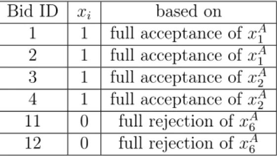
As can be seen in Figure 2 we partially accept the A3 aggregated demand bid. Thus, the set of the three distinguished aggregated bids defined in subsection 2.3 will be A3, A4 and A5 (see Figure 3) – the acceptance indicators of the components of these bids (regarding original bid IDs: 5,6,7,8,9,10) will serve as variables of the second clearing step, while the acceptance of all other original bids are fixed according to the resulting acceptance of the aggregated bid including them as summarized in Table 7.

Bid ID x_i based on 1 1 full acceptance of x^A₁ 2 1 full acceptance of x^A₁ 3 1 full acceptance of x^A₂ 4 1 full acceptance of x^A₂ 11 0 full rejection ofx^A₆ 12 0 full rejection ofx^A₆

Table 7: Fixed variables regarding the acceptance indicators of the original problem.

After this, we perform the second optimization with the remaining original bids (Tables 8 and 9) can be seen in Figure 4.

Bid ID Q[M W h] P [EUR/M W h]

5 91 45

6 90 42

Table 8: Remaining demand offers

As mentioned earlier, fixing the acceptance indicators of bids not corresponding to the three distinguished aggregated bid creates a power imbalance, which must be compensated

Bid ID Q[M W h] P [EUR/M W h]

7 −96 40

8 −71 42

9 −41 47

10 −80 52

Table 9: Remaining supply offers

in the second optimization step. In this example we fix the acceptance indicators of bids 1, 2, 3 and 4 to 1 (see Table 6), resulting in a surplus of

q₁+q₂+q₃+q₄ = 23 + 67 + 27 + 30 = 147M W h

in the demand side, and this has to be taken into account.

The value required to satisfy the power balance constraint calculated above is placed in the appropriate position of the beq vector (its position in the vector is the number of the observed period).

As we need to compensate the demand surplus with production, and supply bids do have a negative sign for quantity, the balance equation for the second optimization is as follows:

91·x5+ 90·x6−96·x7−71·x8−

−41·x9−80·x10=−147.

Figures 3 and 4 depict the remaining aggregated and decomposed offers.

Figure 3: The 3 distinguished aggregated bids, which will be decomposed in the second step.

Solving the second clearing step gives the result (see Figure 4):

Table 10: Bids indicators’ in the second clearing step Bid ID x_i Bid ID x_i

5 0.2198 8 1

6 0 9 0

7 1 10 0

Figure 4: The remaining original bids after the decomposition of the 3 distinguished aggregated bids.

Testing the quantities we get that

x5·q5+x6·q6−x7·q7−

−x₈·q₈−x₉·q₉−x₁₀·q₁₀=

= 0.2198·91 + 0·90−1·96−

−1·71−0·41−0·80 =−147,

the requirement for the power balance is satisfied.

The final result using the results from the first (see Table 7) and the second (see Table 10) steps of optimization:

Table 11: Results with aggregation Bid ID x_i Bid ID x_i

1 1 7 1

2 1 8 1

3 1 9 0

4 1 10 0

5 0.2198 11 0

6 0 12 0

In this case, the results of the original method and the method based on the aggregation of bids are the same. In the following however, we will see that the bid aggregation-based clearing may also induce sub-optimal results in some cases.

3 Results and discussion

In the previous example (2.5), we have always grouped 2 bids into an aggregated bid (thus n was equal to 2), but for larger problems, aggregating a low number of bids does not results in the most efficient solution because the time needed for the first optimization step will be higher due to the large number of aggregated bids.

If we perform the aggregation for flexible number of bids, taking into account their price parameters, we potentially get an aggregated bid set with more equidistant distribution

in the price space, which is beneficial for optimization purposes. We will call the proposed method nominal aggregation.

Although in the majority of the tested scenarios the nominal aggregation based clearing reaches the same TSW as the non-aggregated clearing (thus the result is optimal), in some cases a sub-optimal solution is reached. It is possible, that the decomposition of aggregated bids not fixed after the first clearing step results in a bid set, which can not lead to an optimal solution.

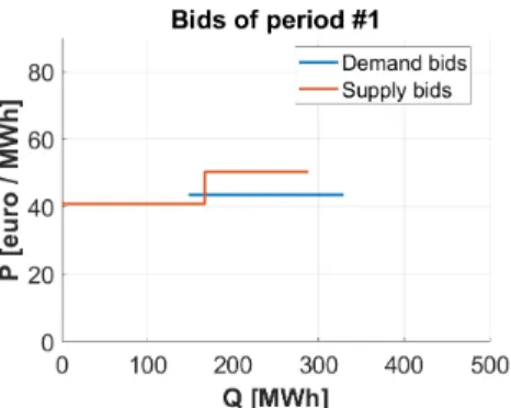
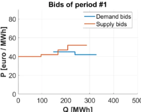
Figures 5 and 6 illustrate such a case: The remaining 3 aggregated bids and the initial bids contained by them are depicted in the figures.

0 100 200 300

Q [MWh]

0 20 40 60 80

P [euro / MWh]

Bids of period #1 Demand bids Supply bids

Figure 5: The 3 distinguished aggregated bids, which will be decomposed in the second step.

0 100 200 300

Q [MWh]

0 20 40 60 80

P [euro / MWh]

Bids of period #1 Demand bids Supply bids

Figure 6: The remaining original bids after the decomposition of the 3 distinguished aggregated bids.

As can be seen on Fig. 5 the curve of the aggregated supply bid meets with the aggregated demand curve (this is the reason why these three aggregated bids were chosen to participate in the second optimization). However in Fig. 6 the supply and demand curves after the decomposition do not intersect each other. If we do not use bid aggregation and solve the original problem, in the TSW maximizing solution, bid 13 is accepted partially.

In contrast, using bid aggregation, its acceptance indicator will be fixed to 0 (according to the acceptance indicators of aggregated offers). From this, it can be clearly seen that the optimal solution can not be reached here via the bid aggregation method.

3.1 Optimality performance

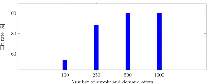
Figures 7 and 8 depict the suboptimality of the aggregation-based method with the number of bids on the x-axis. We examined the results in 250 randomly generated test cases using a predetermined threshold (ε), assuming various number of bids and varying penetration of block bids in the market. If the relative deviation of the TSW value obtained by the actual aggregation method was less then ε, we considered the clearing successful. The maximum of the nominal aggregation’s average relative difference from the reference values was 0.3422% (It occured when the number of supply-demand bids was 100 and the ratio of block bids was 20%.).

100 250 500 1000

60 80 100

Number of supply and demand offers

Hitrate[%]

Figure 7: Optimality of the aggregation based method with ε = 0.1% threshold over 5 time periods. The number of block bids was 10% of the number of supply-demand offers.

100 250 500 1000

60 80 100

Number of supply and demand offers

Hitrate[%]

Figure 8: Optimality of the aggregation based method with ε = 0.1% threshold over 5 time periods. The number of block bids was 20% of the number of supply-demand offers.

According to several tests, as the number of bids increases, the success rates also

show an increasing trend (reaches nearly optimum) and the average relative deviation of TSW values decrease in the case of the nominal aggregation based method. This can be explained by the fact that for multiple bids, the clustering algorithm that determines the original bids to be aggregated into a single bid result in larger clusters. When these larger clusters are decomposed, more bids are available for the algorithm in the second step to optimize, thus the chance is lower to reach sub-optimal result.

3.2 Computational improvement

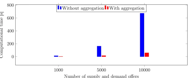
Figures 9 and 10 depict the computational time for different market configurations. In real markets, it is usual to have thousands of offers submitted for a single hour (see e.g.

[6]).

1000 5000 10000

0 200 400 600 800

Number of supply and demand offers

Computationaltime[s]

Without aggregation With aggregation

Figure 9: Computational time for different bid numbers and solution methods over 10 time periods. The number of block bids was 5% of the number of supply-demand offers.

The aggregation based method is faster than the original method by 85%, 91%, 91%

for the increasing bid numbers, respectively.

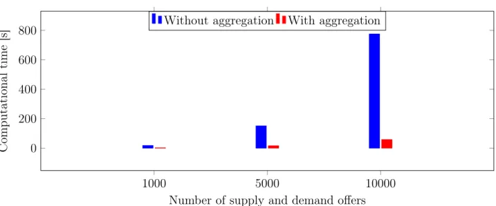
The aggregation based method is faster than the original method by 89%, 90%, 92%

for the increasing bid numbers, respectively.

It is noticeable that with the increase in the number of bids, the aggregation based method outperforms the the standard method used as reference in terms of time require- ment.

The figures also show that the amount of block bids slightly influences the optimization time of the nominally aggregated bids. This can be explained by the fact that block bids are not subject to aggregation. In addition, block bids induce binary variables in the problem, which increase the computational time.

4 Conclusions and future work

In this work we proposed an approximation-based approach for the clearing of electricity markets. The principle of the approach is the concept of bid-aggregation. We analyzed the computational gain and optimality of the method in different scenarios regarding the

1000 5000 10000 0

200 400 600 800

Number of supply and demand offers

Computationaltime[s]

Without aggregation With aggregation

Figure 10: Computational time for different bid numbers and solution methods over 10 time periods. The number of block bids was 10% of the number of supply-demand offers.

number of submitted bids and the ratio of block bids among them. Regarding the computa- tional gain, we found that in the case of large bid quantities the method reduced the compu- tational time by one order of magnitude. Corresponding to the optimality/suboptimality of the proposed method, the results showed that if we assume a large number of bids, the error of the approximation is practically always below 0.5 percent, and if the number of bids was at least 1000-1000 (supply and demand), the error of approximation was below 0.1% in 99% of the simulated cases.

4.1 Future work

In the future we plan to carry out more simulations to evaluate further details of the method. In addition, the current model is TSW-oriented, and does not explicitly consider market clearing prices (MCPs). Introducing MCPs in the model formulation implies im- plication type constraints connecting MCPs and bid acceptance constraints, which may be implemented by the big-M method, implying auxiliary binary variables (see e.g. [7]).

We expect that the proposed method may be applied efficiently in this case as well, based on the consideration that the significant reduction of bid number leads to the reduction of the number of these auxiliary binary variables.

As mentioned earlier, clearing based on the aggregation of bids can potentially reach a sub-optimal solution. To overcome this issue the algorithm may be initiated with several possible aggregation configurations and the version with the highest TSW value may be considered as the final solution. The optimization problems resulting from these different initial aggregation scenarios may be evaluated in a parallel manner.

5 Acknowledgements

This work has been supported by the Integrated researcher training program in the dis- ciplines of information technology and computer science (EFOP-3.6.3-VEKOP-16-2017- 00002) project, and by the Funds PD 123900 and K 131545 of the Hungarian National

Research, Development and Innovation Office. D{avid Csercsik is the grantee of the János Bolyai Research Scholarship of the Hungarian Academy of Sciences.

Bibliography References

[1] M. Madani, Revisiting european day-ahead electricity market auctions: Mip models and algorithms, PhD Thesis, Universite Catholique de Louvain (2017).

[2] M. Madani, M. Van Vyve, A. Marien, M. Maenhoudt, P. Luickx, A. Tirez, Non- convexities in european day-ahead electricity markets: Belgium as a case study, in:

2016 13th International Conference on the European Energy Market (EEM), IEEE, 2016, pp. 1–5.

[3] Á. Sleisz, D. Divényi, D. Raisz, New formulation of power plants’ general complex orders on european electricity markets, Electric Power Systems Research 169 (2019) 229–240.

[4] L. Meeus, K. Verhaegen, R. Belmans, Block order restrictions in combinatorial electric energy auctions, European journal of operational research 196 (3) (2009) 1202–1206.

[5] Euphemia public description, Tech. rep., accessed on 12/11/2019 (2015).

URLhttp://www.belpex.be/wp-content/uploads/Euphemia-public-description-Nov-2013.

pdf

[6] Hupx dam monthly report march 2019,

https://hupx.hu/hu/, Tech. rep., accessed on 12/11/2019 (2019).

URL https://hupx.hu/uploads/Piaci%20adatok/DAM/havi/2019/HUPX_DAM_OLAP_

Monthly_external_4MMC_Mar.pdf

[7] D. Csercsik, Á. Sleisz, P. M. Sőrés, The uncertain bidder pays principle and its im- plementation in a simple integrated portfolio-bidding energy-reserve market model, Energies 12 (15) (2019) 2957.