Treatment Oka OF

(1)

THE PRINCIPLES OF RHEOMETRY S. Oka

I. Introduction 18 II. Capillary Viscometers 21

1. Non-Newtonian Flow 21 2. Materials with Specified Flow Behavior 23

a. Newtonian Liquids 24 (1) End-Effect 24 (2) Kinetic Energy Correction 24

b. Bingham Solids 25 c. Power Law Flow Curve 28

(1) de Waele-Ostwald's Law 28 d. Development of /(r) into Taylor's Series 28

e. Ferry's Flow Law 29 3. Apparent Fluidity 29 III. Rotating Coaxial Cylinder Viscometers 29

1. Inelastic Liquids of Arbitrary Flow Curve 29 2. Liquids with Specified Flow Curve 32

a. Newtonian Liquids 32 b. Bingham Solids 33 c. Power Law Flow Curve (de Waele-Ostwald's Law) 34

d. Development of /(r) into Taylor's Series 34

e. Ferry's Flow Law 34 3. Apparent Fluidity 34 4. Hydrodynamic Treatment 36

5. End-Effect 37 a. Theory of the End-Effect for Plane Ends 37

6. Viscoelastic Liquids 40 IV. Oscillating Coaxial Cylinder Viscometers 42

1. Forced Oscillations 42

2. End-Effect 47 3. Free Oscillations •· · 48

4. Outer Cylinder in Oscillation 49

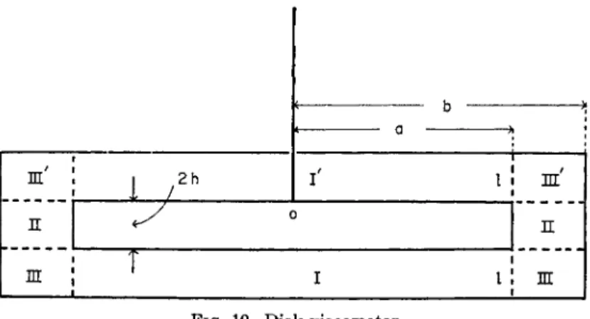
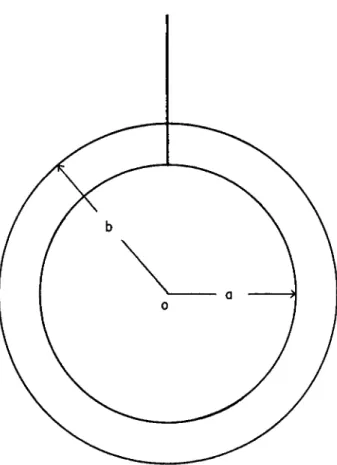
V. Disk Viscometers 51 1. Rotating Disk Viscometers 51

2. Oscillating Disk Viscometers: Free Oscillations 53

a. General Case 54 b. Special Case 55 VI. Concentric Sphere Viscometers 56

1. Rotating Concentric Sphere Viscometers 56 17

(2)

18 ^{S. OKA}

2. Oscillating Concentric Sphere Viscometers 58

a. Forced Oscillations 58 b. Free Oscillations 60 VII. Cone and Plate, Double Cone, and Conicylindrical Viscometers 61

1. Cone and Plate Viscometers 61 2. Double Cone Viscometers 62 3. Conicylindrical Viscometers 63 VIII. Oscillating Plate Viscometers 65

1. Newtonian Liquids 65 2. Edge-Effect 67 3. Wall-Effect 68 IX. Falling Sphere Viscometers 70

1. Stokes'Law 70 2. Corrections for Stokes' Law 71

a. Effect of Finite Reynolds' Number 71

b. Wall-Effect 71 c. End-Effect 73 X . Parallel Plate Plastometers 73

1. Newtonian Liquids 73 2. Linear Viscoelastic Bodies 75 3. Non-Newtonian Liquids 76 X I . Coaxial Cylinder Viscometers with Axial Motion 77

1. Pochettino Viscometer 77

2. Penetrometer 78 3. Oscillating Penetrometer 79

Nomenclature 80 I. Introduction

This chapter is concerned with methods for determining the rheological properties of liquids and gases. W e will deal mostly with inelastic incom- pressible fluids manifesting Newtonian flow behavior, that is, with materials the rheological properties of which are characterized b y a single parameter for isothermal conditions, as discussed in Chapter 16 of Volume I. M a n y such methods involve measurements of the motion of one surface in con- tact with the liquid relative to another surface. In the case of liquids of low viscosity, one of these surfaces is in the form of a container to hold the liquid. T h e surfaces m a y be effectively at an infinite distance from each other.

T h e rheological behavior of a Newtonian liquid in an appropriate instrument is obtained in principle b y solution of the Navier-Stokes equation for the appropriate boundary conditions. Owing to the existence of a quadratic term in this equation, exact solutions cannot in general be obtained. If the quadratic term is dropped, solutions thus obtained are approximate except in the limiting case of infinitesimally slow motion. T h e quadratic term corresponds physically to a secondary flow superimposed upon the

(3)

flow derived from the simplified Navier-Stokes equation. T h e solutions discussed in this chapter are obtained from linearized forms of the Navier- Stokes equation and must be considered to a certain extent approximate, except when quadratic terms vanish identically, as in capillary flow. Some discussion of secondary flow has recently appeared in the literature.

Relatively simple results in closed form for the simplified equation can be obtained in general only with certain geometries. In many cases an experimentally convenient form of apparatus is not tractable mathematically.

In such circumstances it is customary to obtain solutions for simplified geometries and then to apply empirical or calculated corrections for so- called "end-effects," "edge-effects," and "wall-effects." In this chapter some formal solutions are given for certain rheological instruments with such experimentally convenient geometries. Numerical calculation from the analyses of correction terms m a y be more or less difficult. Unfortu- nately, some of these formal solutions are so untractable that they can b e regarded as little more than reformulations of the problem. T h e y m a y , however, indicate convenient approximations for particular cases.

This chapter is also concerned with the measurement of the rheological properties of materials manifesting linear viscoelastic behavior. Formally, such behavior m a y be characterized b y a linearized Navier-Stokes equation, or the generalized H o o k e ' s law equation with a " m e m o r y ' term. In practice, we will deal mostly with sinusoidally varying stress or strain, under which condition it is customary merely to consider the viscosity or elasticity as complex; this procedure is, however, not strictly justified for resonance methods, since the complex viscosity or elasticity is a function of frequency.

Finally, we consider the steady flow behavior of materials manifesting non-Newtonian behavior. F o r such behavior the shear stress in steady rectilinear flow is a single-valued monotonically increasing function of the rate of shear, the so-called "flow c u r v e " ; thixotropic behavior is thus ex- cluded. Non-Newtonian flow behavior is characterized not only b y the shear stress at a given rate of shear under such a flow pattern, but also b y the nonzero differences in stresses which act normally on the three mutually perpendicular planes associated with flow. These normal stresses are n o t considered in this chapter.

T h e main objective of this chapter is thus to give results for the above types of flow behavior for certain of the more usual geometries, and to show the mathematical procedures involved. For completeness, well-known results for several other arrangements are included. M a n y variations of the arrangements discussed are possible. Space does not permit the description or listing of these variations; however, from the mathematical procedures given for the typical methods discussed here, the alternative arrangements

(4)

TABLE I

CASES DISCUSSED IN THIS CHAPTER

Type of instruments Type of motion Rheological properties Effects considered Capillary viscometer Rectilinear flow Newtonian

Non-Newtonian Linear viscoelastic

End-effect No end-effect End-effect Rotating coaxial

cylinder viscometer

Rotation Newtonian Non-Newtonian Linear viscoelastic

End-effect No end-effect End-effect Oscillating coaxial

cylinder viscometer

Forced oscillation Linear viscoelastic 1

Newtonian / End-effect

Oscillating coaxial cylinder viscometer

Free oscillation Linear viscoelastic 1

Newtonian / No end-effect

Rotating disk viscometer

Rotation

Newtonian [Edge-effect j End-effect

[Wall-effect Oscillating disk vis-

cometer

Free oscillation

Newtonian [Edge-effect j End-effect

[Wall-effect Rotating concentric

sphere viscometer

Rotation Newtonian Wall-effect

Oscillating concentric sphere viscometer

Forced oscillation ÎLinear viscoelastic 1

\Newtonian J Wall-effect

Oscillating concentric sphere viscometer

Free oscillation ÎLinear viscoelastic 1

(Newtonian j Wall-effect

Cone and plate vis-

cometer Rotation [Newtonian ]

j Non-Newtonian >

[Linear viscoelastic J No edge-effect Double cone vis-

cometer Rotation (Newtonian 1 (Linear viscoelastic J No edge-effect Conicylindrical vis-

cometer Rotation [Newtonian ]

\ Non-Newtonian >

[Linear viscoelastic J

No edge-effect No corner-effect Oscillating plate

viscometer Forced oscillation ÎNewtonian

(Linear viscoelastic Edge-effect Wall-effect 20

(5)

TABLE 1—(CONTINUED)

TYPE OF INSTRUMENTS TYPE OF MOTION RHEOLOGICAL PROPERTIES EFFECTS CONSIDERED Falling sphere vis-

cometer

Rectilinear motion Newtonian ÎWall-effect

\End-effect Parallel plate plas-

tometer

Compression [Newtonian ]

\ Non-Newtonian >

[Linear viscoelastic J

No edge-effect

Pochettino viscometer

Rectilinear motion ( Newtonian \

\Linear viscoelastic J No end-effect Penetrometer Rectilinear motion Newtonian No end-effect Oscillating pene-

trometer

Axial oscillation [Linear viscoelastic 1

\Newtonian / No end-effect

can be treated similarly. Since this chapter is concerned only with mathe- matical relationships between instrument geometry, observable quantities, and rheological properties, no discussion is given of the scope of each ar- rangement or of experimental details.

Strictly speaking, the three types of flow behavior considered here, namely, inelastic Newtonian behavior, inelastic non-Newtonian flow, and linear viscoelastic behavior, represent the flow behavior of real liquids only under limiting conditions. In practice, the rheological behavior of a liquid in a given instrument under given conditions may approximate one of these idealized types, and this can be determined by varying the experimental conditions. The cases discussed in this chapter are listed in Table I.

II. Capillary Viscometers

1. NO N -NE W T O N I A N FL O W

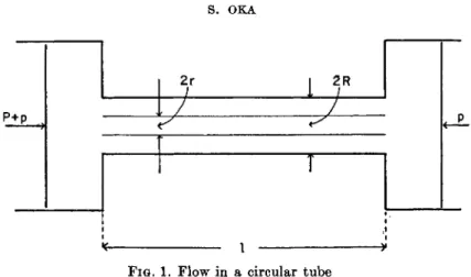
Let us consider the flow of an incompressible liquid through a circular tube, of radius R and length Z, as shown in Fig. 1. At each end of the tube are reservoirs, containing pistons exerting pressures Ρ + ρ and ρ respec- tively. In practice Ρ may be a hydrostatic head, and ρ atmospheric pressure.

The tube and reservoirs are the fixed member, and the pistons the movable member. Let Q be the volume of flow in unit time. The rheological behavior of the liquid is specified by the flow curve

7 = /(r), (1)

where y is the rate of shear, which is equal to the velocity gradient for rec-

(6)

2 2 S. OKA

±

2R ^{2 R}

l

FIG. 1. Flow in a circular tube

TILINEAR FLOW, AND R IS THE SHEAR STRESS. F R O M THE MEASUREMENT OF THE RELA- TION BETWEEN Ρ AND Q THE FLOW CURVE M A Y BE DETERMINED. W I T H REGARD TO THE MOTION OF THE LIQUID, THE FOLLOWING ASSUMPTIONS ARE M A D E : ( I ) THE LIQUID IS INCOMPRESSIBLE; (II) THE MOTION OF THE LIQUID IS NOT TURBULENT; (III) THE STREAMLINES ARE PARALLEL TO THE AXIS OF THE TUBE; THAT IS, THE LIQUID IS "TELE- SCOPING" THROUGH THE TUBE; ( I V ) THE MOTION IS STATIONARY; ( V ) THERE IS NO SLIP AT THE WALL. W E WILL CONSIDER FIRST THE BEHAVIOR OF THE CAPILLARY VISCOME- TER WITH LIQUIDS OF ARBITRARY FLOW CURVE, AND SUBSEQUENTLY WITH LIQUIDS OF SPECIFIED FLOW BEHAVIOR.

LET US CONSIDER THE CYLINDRICAL SURFACE IN THE LIQUID OF RADIUS r AND OF LENGTH I AS IN F I G . 1. IF WE DENOTE THE LONGITUDINAL SHEAR STRESS ACTING ON THE CYLINDRICAL SURFACE B Y R, THEN THE RESULTANT FORCE ARISING FROM THE LONGITU- DINAL TRACTIONS ON THE CYLINDRICAL SURFACE BECOMES 2πήτ. N O W FOR BOTH M A - TERIALS MANIFESTING NEWTONIAN AS WELL AS NON-NEWTONIAN FLOW BEHAVIOR,1

THE DIFFERENCE Ρ IN AXIAL NORMAL STRESS IS INDEPENDENT OF r (ASSUMPTION III).

A S A CONSEQUENCE OF THE ASSUMPTION ( I V ) , THE FORCE MUST BE EQUAL TO THE NET DRIVING FORCE

irr

²

P.

HENCE WE HAVE 2πΗτ

= πτ

²

Ρ,

OR2

R = (P/2l)r ( 2 )

IF WE DENOTE THE VELOCITY OF THE LIQUID AT A DISTANCE r FROM THE AXIS OF THE TUBE B Y v(r), THE RATE OF SHEAR IS GIVEN B Y —dv/dr, AND THE VOLUME OF FLOW IN UNIT TIME IS GIVEN B Y

**Q = f* 2irrv(r) dr = | ττΛ |**

⁰

* - f* irr

²

^ dr

Jo Jo dr

T H E FIRST TERM ON THE RIGHT-HAND SIDE VANISHES, BECAUSE, FROM ASSUMPTION

1 R. S. Riwlin, Proc. Cambridge Phil. Soc. 45, 88 (1948).

2 This equation was first derived by G. G. Stokes in 1851.

(7)

( v ) ,

v(R)

must be zero. Substituting

—dv/dr

= / ( r ) into the a b o v e equation and changing the variable of integration from r to τ, we h a v e3 ,4

where

TB =

PR/21

(4)

denotes the shear stress at the wall. Thus we see that the quantity 4Q/7TÄ3

is a function of r^R only.

T h e relation between Ρ and Q, that is, between rR and Dy can be directly observed. W e need only find the flow curve / ( τ ) from the known function D(TR). Cancelling the denominator of equation (3) and differentiating with respect to r^R , we obtain

f(r

^R

) = \D{r

^R

) +

^\T^rD\TR)

where

D

^f

= dD/dr.

Since this relation must hold for any value of

r

^R , we shall simply write τ for rR . Thus we have the result³*⁴:

/ ( r ) = iD(r) + JTZ)'(T) (5) F r o m equations (1) and (2) it can be seen that the relation between the

rate of shear and the distance r from the axis of the tube is given b y

Thus the rate of shear increases from zero to a maximum f(rR) with increase in r from zero to Ä . In capillary viscometers the rate of shear cannot be regarded as uniform.

Integration of the equation

—dv/dr

= / ( r ) leads to the distribution of the velocity

ν = -Γΐ{τ)άτ ( 6 )

TR JT

2. M A T E R I A L S W I T H SPECIFIED F L O W B E H A V I O R

If conditions (i) to ( v ) are complied with, then y as a function of τ is obtained from equation ( 5 ) . T h e alternative procedure is t o

assume

a reasonable flow law, and compare the observed Q-P curve with the curve calculated according to the law. W e will n o w give some examples of Q-P curves for various flow laws.

3B . Rabinowitsch, Z. physik. Chem. (Leipzig) A145, 1 (1929).

4 M. Reiner, "Deformation and Flow," p. 108. Lewis, London, 1949.

(8)

24 S. O K A

α. Newtonian Liquids

A Newtonian liquid is specified b y the flow curve

fir) = τ/η, (7) where η is the coefficient of viscosity. Substituting the a b o v e relation for

equation (3) gives

D(TR)

= τκ/η

Expressing this relation in terms of Q and P , we get the well-known Hagen- Poiseuille equation

Q = (^νϋ^Α/81η)Ρ (8)

It can be seen from equation (6) that the distribution of velocity across the tube is parabolic :

. - « • - . - > £

Since the assumptions in the previous subsection d o not hold in actual capillary viscometers, it becomes necessary to correct the Hagen-Poiseuille equation for certain effects. Here, we will briefly mention only end-effect and kinetic energy corrections.

(1) End-effect. Since the ends of the capillary tube are connected with wide vessels, the streamlines are not completely parallel to the axis near the end of the tube. For this reason, the velocity of the liquid in the direc- tion of the axis near the end is less than that in the middle part of the tube.

Hence the end-effect m a y be considered as equivalent to an increase in the effective length of the capillary tube from I to I + ΔΖ. T h e correction Al is sometimes called the Couette correction; it is usually written in the form Al = nR, but n is variously evaluated. Rayleigh gives 0.824; Scheader, 0.805; and B o n d , 0.566.

(2) Kinetic energy correction. W h e n the liquid which is m o v i n g slowly along the wide tube suddenly finds itself in the capillary tube, it has t o m o v e much more quickly, and therefore the pressure falls. T h e effective pressure difference is smaller than the measured one. Let ν — Q/wR² denote the average velocity and ρ the density of the liquid. T h e n this behavior corresponds to substituting Ρ — mpv² for Ρ in the Hagen-Poiseuille equation. Consequently we have

wR*P mpQ

v = _{SIQ Swl}

This correction is sometimes called the Hagenbach correction, and the numerical factor m has been variously evaluated as in Table I I .

(9)

T A B L E I P

VALUES OF m ACCORDING TO SEVERAL AUTHORS

Reynolds 0 . 5 0

Hagenbach 0 . 7 9

Couette and (independently) Wilberforce 1.00

Boussinesq 1.12

Riemann 1.124

Swindells 1 . 1 2 - 1 . 1 7

Knobbs 1.14

Jacobson 1 . 2 5 - 1 . 5 5

T h e Hagen-Poiseuille equation, corrected both for the end-effect and for the kinetic energy, m a y be written

= *R*P _ rnpQ , ν

η SQ(l + nR) SV(Z + n ß ) w

For experimental determination of the constants m and η the reader should refer t o the paper of Swindells.6

b. Bingham Solids

Bingham solids are defined b y the relation:

/(,)-»

^to

,

^Sr

,|

Sir) = (l/i/pi)(r - r,) for r > r, ,)

where 77 is the yield value and 77^1 is the plastic viscosity. Thus the Bingham solid is specified b y t w o material constants r/ and r/pi, which are t o be determined. T w o cases m a y be distinguished.

(i) rR < TF, that is, Ρ < 2lrf/R, since rR = PR/21. From physical considerations it is expected that there will be no flow in this case. This can also be verified from equation ( 3 ) , since D(rR) becomes zero when TR

< Tf .

(ii) TR > τ/ , that is, Ρ > 2lrf/R. W e get from equation (3)

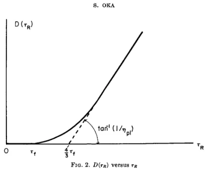
D(rR) = λ [ Τ Λ- * + \ ΐ ζ \ (11)

Vpi L 3 3 r^{Ä 3}

J

F r o m the a b o v e considerations, the relation between D(TR) and rR is as in Fig. 2. T h e curve touches the abscissa at TR = 77 and begins to rise at TR = Tf ; the intersection of the asymptote and the abscissa is given b y

6 A. C. Merrington, "Viscometry." Arnold, London, 1949.

8 J. F. Swindells, J. R. Coe, Jr., and T . B. Godfrey, J . Research Natl. Bur. Stand- ards 48, 1 (1952).

(10)

26

^{S. O K A}

0

FIG. 2. D(TR) versus r^R

TR = · Then ηρι may be calculated from the slope of the asymptote.

Equation (11) may be written in terms of Ρ and Q as follows:

where

ρ

=

2lr//R.

This is the

Buckingham-Reiner equation,7'8

which, when Tf = 0, reduces of course to the Hagen-Poiseuille equation.

We will now proceed to discuss the distribution of velocity on the basis of equation (6) for the case when r

^R > r^s

. When τ < τ/ , that is, when

r is less than a critical value r^c

given by

we have from equation (6)

Thus the velocity is constant and independent of r if r does not exceed the critical radius r

^c

. When r > r/ , that is, r > r

^c

, we have

From the above considerations, the distribution of velocity is as in Fig. 3.

Thus the cylindrical portion of radius r moves as if it were rigid. This type of flow is called

plug flow.

7 E. Buckingham, Am. Soc. Testing Materials, Proc. 2 1 , 1154 (1921).

8 M. Reiner, Kolloid-Z. 39, 80 (1926).

(12)

r

^c

= Ä(r//r

^Ä

),

ν = (P/4fy^{p l}

)[Ä

²

- r

²

- 2r

^c

(ß - r)]

²

(11)

1

2 R

^ >

2 R 2 R 2 R

Τ

FIG. 3. Plug flow in a circular tube.

Q

Ο Ρ 4

"SP

FIG. 4. Volume of flow in unit time Q versus the pressure difference Ρ W h e n there is a slip at the wall, we must add v^R , the velocity of the material at the wall, to the right-hand side of equation (6) ; that is, a term TR2VR must be added to the right-hand side of equation (12). Let us assume that there is a very thin lubricating layer of thickness e next to the capillary wall. T h e shear stress T^R = PR/21 at the wall divided b y the viscosity coefficient 171 of the lubricating layer is equal to the velocity gradient v^R/e'^y hence, we have

vR = ePR/2LM

Adding this term to the right-hand side of equation (12), we g e t^{9 , 10}

W Sk»i L 3^V ^ 3 P³J 2L^{M R}

The relation between Q and Ρ is shown in Fig. 4. Q first increases linearly

9 M. Reiner, "Deformation and Flow." Lewis, London, 1949.

1 0 G. Green, "Industrial Rheology and Rheological Structures," p. 26-27. Wiley, New York, 1949.

(12)

28 S. OKA

with increase in Ρ and begins to rise more steeply at Ρ = p. T h e intersection of the asymptote and the straight line O A corresponds to

Ρ

=

($i)p.

Thus e/ηι m a y be obtained from the slope of the straight line O A , 77 from the relation ρ = 2Zr//Ä, and the plastic viscosity η^ρι from the slope of the asymptote.

c. Power Law Flow Curve

Let us consider the flow curve given b y

/ ( τ ) = 0 for r < Tf , / ( R ) = ( L / * ) ( R - T , ) « f o r τ > R ,

This is

Herschel-Bulkley's law

^y and the special case

n

= 1 corresponds to the Bingham solid. It is noticed that the dimensions of k differ in general from those of the coefficient of viscosity. In this case also, no flow occurs when

tr < τ/

^y that is,

Ρ < 2lr

^f

/R.

This is also clear from equation ( 3 ) . W h e n tr > τ/ , we obtain

(η + 3)fc \

tr) L

η + 3 rÄ

1 (η + 2 ) ( n + 3)

\t

^r

and τ/ is obtained from the point at which the curve of D(t^r) touches the abscissa. Thus, if we assume Herschel-Bulkley's law, n and k m a y be o b - tained from the above relation.

(1)

de Waele-Ostwald's law.

W e will examine the special case when Tf = 0, that is, the case for quasi-viscous flow

( 1 / * ) T »

Q =

V (n + 3 ) * \

21 J

⁷

which reduces to the Hagen-Poiseuille equation when n = 1. T h e a b o v e formula was first derived b y Farrow et al.11

d. Development of / ( r ) into Taylor

⁹

s Series

Let us consider t h a t / ( r ) is developed into power series of τ — r/ , where Tf is the yield value. It m a y be argued that in the series of / ( r ) / ( r — τ/) all terms with o d d powers of r — 1/ should vanish, b e c a u s e / ( r ) / ( r — τ/) corresponds to the fluidity and accordingly it does not change its sign with the change of sign of r — r/ .1 2 If we substitute the series for / ( r ) into

11 F. D. Farrow, G. M. Lowe, and S. M. Neale,

J. Textile Inst. Trans.

^19, 18 (1928).

1 2 M. Reiner, "Twelve Lectures on Theoretical Rheology,'' p. 133. North-Holland, Amsterdam, 1949.

T h e n we obtain

(η + 3)fc '

(13)

EQUATION ( 3 ) , WE GET AN EXPRESSION FOR D ( RÄ) , FROM WHICH / ( Τ ) M A Y BE DE- TERMINED.

FOR MATERIALS FOLLOWING FLOW LAWS OF OTHER TYPES THE READER SHOULD REFER TO THE TABLE OF PHILIPPOFF'S B O O K .13

E. Ferry's Flow Law

T H E FLOW BEHAVIOR OF POLYMERIC SYSTEMS AT VERY LOW RATES OF SHEAR APPEARS TO BE IN GOOD AGREEMENT WITH THE EMPIRICAL EQUATION PROPOSED B Y F E R R Y :14

7

= / W

= ( R / * ) [ L +

(τ/Gi)],

^{( 1 4 )}

WHERE η IS THE VISCOSITY DEFINED AS THE LIMITING VALUE OF Τ / Γ , AND G » IS A CONSTANT OF THE DIMENSIONS OF STRESS; FOLLOWING FERRY, THIS CONSTANT IS CALLED THE

internal shear modulus.

INSERTING EQUATION ( 1 4 ) INTO EQUATION ( 3 ) WE OBTAIN

3 . A P P A R E N T F L U I D I T Y

I N NEWTONIAN LIQUIDS THE FLUIDITY <p, THE RECIPROCAL OF THE COEFFICIENT OF VISCOSITY, IS GIVEN B Y D(TR)/TR AS SHOWN IN SECTION I I , 2 , A . T H I S QUANTITY IS NOT CONSTANT IN THE CASE OF NON-NEWTONIAN LIQUIDS; HOWEVER, IT HAS THE DIMENSIONS OF FLUIDITY. T H U S , FOR THE CAPILLARY VISCOMETER WE M A Y DEFINE AN APPARENT FLUIDITY GIVEN B Y

<pc = D(TR)/TR

T H E N THE RELATION

KTR) = ÏD(T^r) + IT^rD'(TR)

M A Y BE WRITTEN IN TERMS OF <pc AS FOLLOWS:15

A N D / ( TÄ) / TÄ IS THE APPARENT FLUIDITY φ^α AS USUALLY DEFINED. FOR NEWTONIAN LIQUIDS

<p

^c IS CONSTANT A N D / ( RÄ) =

φ

⁰

τ

^κ . T H E SECOND TERM IN THE BRACKET OF EQUATION ( 1 5 ) REPRESENTS THE DEVIATION FROM NEWTONIAN FLOW.

III. ROTATING COAXIAL CYLINDER VISCOMETERS

1. I N E L A S T I C L I Q U I D S OF A R B I T R A R Y F L O W C U R V E

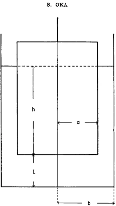
I N THE ROTATING CYLINDER VISCOMETER, A LIQUID IS PLACED IN THE ANNULAR SPACE BETWEEN TWO COAXIAL CYLINDERS, AS IN F I G . 5 . O N E OF THE CYLINDERS IS FIXED,

1 3 W. Philippoff "Viskosität der Kolloide," p. 46. Steinkopff, Leipzig, 1942.

14 J. D. Ferry,

Am. Chem. Soc.

^64, 1330 (1942).

1 61 . M . Krieger and S. H. Maron,

J. Appl. Phys.

^{2 3 ,} 147, 1412 (1952).

(14)

30

^{S. O K A}

f

ζ α i

ι

ι I I I

it

^b

ï

FIG. 5. Coaxial cylinder viscometer

w h i l e t o t h e o t h e r i s a p p l i e d a t o r q u e M. W e w i l l c o n s i d e r t h e p e r f o r m a n c e o f s u c h a n i n s t r u m e n t w h e n M i s a c o n s t a n t . L e t Ω b e t h e a n g u l a r v e l o c i t y û o f t h e c y l i n d e r a f t e r r e a c h i n g a s t a t i o n a r y s t a t e . F r o m t h e m e a s u r e m e n t o f t h e r e l a t i o n b e t w e e n Ω a n d M, t h e flow c u r v e o f t h e l i q u i d m a y b e d e t e r - m i n e d . T h i s s i t u a t i o n c o r r e s p o n d s t o t h e d e t e r m i n a t i o n o f t h e flow c u r v e f r o m t h e r e l a t i o n b e t w e e n Q a n d Ρ i n c a p i l l a r y v i s c o m e t e r s . W e w i l l first c o n s i d e r i n e l a s t i c l i q u i d s o f a r b i t r a r y flow c u r v e y = / ( τ ) , a n d s u b s e q u e n t l y i n e l a s t i c l i q u i d s w i t h s p e c i f i e d flow b e h a v i o r . F i n a l l y , t h e e f f e c t o f t h e e n d w i t h t h e g e o m e t r y o f F i g . 5 w i l l b e c o n s i d e r e d f o r a N e w t o n i a n l i q u i d , a n d a l s o f o r a l i q u i d m a n i f e s t i n g l i n e a r v i s c o e l a s t i c b e h a v i o r .

W i t h r e g a r d t o t h e m o t i o n o f t h e l i q u i d , t h e f o l l o w i n g a s s u m p t i o n s a r e m a d e : ( i ) t h e l i q u i d i s i n c o m p r e s s i b l e ; ( i i ) t h e m o t i o n o f t h e l i q u i d i s n o t t u r b u l e n t ; ( i i i ) t h e s t r e a m l i n e s a r e c i r c l e s o n t h e h o r i z o n t a l p l a n e s p e r - p e n d i c u l a r t o t h e a x i s o f r o t a t i o n ; ( i v ) t h e m o t i o n i s s t a t i o n a r y ; ( v ) t h e r e i s n o r e l a t i v e m o t i o n b e t w e e n t h e c y l i n d e r s a n d t h e m a t e r i a l i n i m m e d i a t e c o n t a c t w i t h t h e c y l i n d e r s ; a n d ( v i ) t h e m o t i o n o f t h e l i q u i d i s t h e s a m e o n e a c h p l a n e p e r p e n d i c u l a r t o t h e a x i s o f r o t a t i o n ; t h a t i s , t h e m o t i o n i s t w o - d i m e n s i o n a l . A s s u m p t i o n ( i i i ) c o r r e s p o n d s t o n e g l e c t i n g t h e e f f e c t o f

(15)

CENTRIFUGAL FORCES, AND FOR SMALL VALUES OF Ω THIS ASSUMPTION, AS WELL AS ( I I ) , M A Y BE ALLOWED. ASSUMPTION ( V I ) MEANS NEGLECTING THE END-EFFECT.

LET US CONSIDER A CYLINDRICAL SURFACE IN THE LIQUID OF RADIUS r AND OF HEIGHT A. IF WE DENOTE THE TANGENTIAL SHEAR STRESS ON THE CYLINDRICAL SURFACE B Y R, THEN THE RESULTANT M O M E N T ARISING FROM THE TANGENTIAL TRACTIONS ON THE CYLINDRICAL SURFACE BECOMES 2rr2hr. A S A CONSEQUENCE OF ASSUMPTION ( I V ) , THIS M O M E N T MUST BE EQUAL TO THE TORQUE M APPLIED TO THE CYLINDER. HENCE WE HAVE

M = 2wr2hr ( 1 6 )

WHICH CORRESPONDS TO EQUATION ( 2 ) FOR CAPILLARY VISCOMETERS. LET THE RADIUS OF THE INNER CYLINDER BE A, AND THAT OF THE OUTER CYLINDER BE b; LET THE VALUE OF τ AT r = a AND r = b BE τα AND η , RESPECTIVELY. T H E N WE HAVE FROM EQUATION ( 1 6 )

Μ = 2παΗτα = 2wb2hrb ( 1 7 )

LET US NOW IMAGINE THAT THE INNER CYLINDER IS ROTATED WITH A CONSTANT ANGULAR VELOCITY Ω . IF WE DENOTE THE ANGULAR VELOCITY OF THE LIQUID PARTICLES AROUND THE AXIS B Y ω(τ), THEN THE RATE OF SHEAR IS GIVEN B Y

y = — r άω/dr

T H E N WE HAVE FROM EQUATION ( 1 6 )

2R dœ/dr = / ( R ) ,

OR, INTEGRATING UNDER THE BOUNDARY CONDITIONS Ω ( Α ) = Ω AND Ω ( 6 ) = 0 ,

2Jrt r AND

Ο - ! / " * ! * * · ( 1 8 )

EQUATION ( 1 8 ) , WHICH REMAINS UNALTERED WHEN THE OUTER CYLINDER ROTATES AND THE INNER CYLINDER IS FIXED, GIVES THE RELATION BETWEEN Ω AND M CORRE- SPONDS TO EQUATION ( 3 ) FOR CAPILLARY VISCOMETERS.

T H E RELATION BETWEEN THE VELOCITY GRADIENT AND r IS, FROM EQUATION ( 1 6 ) , 7 = f(M/2irr2h)

THEREFORE, y M A Y BE ASSUMED TO BE CONSTANT THROUGHOUT THE LIQUID, pro- vided that THE CLEARANCE IS VERY SMALL, THAT IS, ( 6 — a)/a <3C 1.

N O W THE PROBLEM IS TO FIND THE FLOW CURVE / ( R ) FROM THE KNOWN RELATION BETWEEN Ω AND M. DIFFERENTIATING EQUATION ( 1 8 ) WITH RESPECT TO M AND

(16)

32 s.

O K A

writing g(r

^a) for

we have

2M <Kl/dM = 2τ^α dil/dra

flf(T.) =

f(r^a) - f(s-²r^a)

where s = b/a. From the difference equation the flow curve may be ob- tained in the form

¹⁶

fir) « Σ g(s'²ⁿr) = 2r Σ e ^ o W ) (19)

η—Ο η—0

where Ω' =

dü/dr.

The sum is a slowly convergent one when

s

œ 1, which may be asymptotically evaluated using the Euler-MacLaurin sum for- mula.

¹⁷

There is another method of obtaining/(r) from equation (18). If we set

r^a = s²n and differentiate both sides of the equation with respect to s,

keeping η constant, we get

¹⁵

/(r

^e

) = s(dÜ/ds)

^Tb

(20)

Further discussions for the methods of determination of the flow curve are given in Section 111,3.

2. L I Q U I D S W I T H S P E C I F I E D F L O W B E H A V I O R

An alternative procedure is to assume as before a reasonable flow curve*

and to compare the calculated relation between M and Ω with the observed one.

a. Newtonian Liquids

Substituting τ/η for/(τ) in equation (18), then from equation (17) we obtain

which is the well-known

Margules equation.

This equation corresponds to the Hagen-Poiseuille equation for capillary viscometers. The coefficient of viscosity η is determined from the measurable quantity M/il.

The rate of shear y and its average value 7av are given by

2/r² .

1 2

' (1/α«) - (1/62) - » - v

^b _ α ( 1 / α ) + ( 1 / 6)

respectively. 7av is approximately equal to αΩ/(6 — α), provided that (6 - α) /a « 1.

ι· J. Pawlowski, Kolloid-Z. 130, 129 (1953).

» I. M. Krieger and H. Elrod, / . Appl. Phys. 24, 134 (1953).

(17)

b. Bingham Solids^12,18

T h r e e c a s e s m a y b e d i s t i n g u i s h e d f o r t h e flow b e h a v i o r o f a B i n g h a m s o l i d i n a r o t a t i n g c o a x i a l c y l i n d e r v i s c o m e t e r .

( i ) TA < τ/. I n t h i s c a s e ω i s z e r o t h r o u g h o u t t h e m a t e r i a l a n d Ω = 0 f r o m e q u a t i o n ( 1 8 ) . T h e m a t e r i a l d o e s n o t flow a t a l l .

( i i ) T6 < τ/ < TA . F l o w o c c u r s w h e n τ > τ / . T h e r e f o r e , flow o c c u r s w h e n r i s l e s s t h a n a c r i t i c a l v a l u e rc g i v e n b y

rc = (M/2whT^f)¹¹²

w h i l e n o flow o c c u r s w h e n r i s l a r g e r t h a n rc. T h i s c o r r e s p o n d s t o p l u g flow i n c a p i l l a r y v i s c o m e t e r s . F r o m e q u a t i o n ( 1 8 ) w e h a v e

Ω = (1/2ηρ1)[τα - TS- TF I n ( τα/ τ / ) ] ,

w h i c h h o l d s f o r ra < S2T/ .

( i i i ) τ/ < η . I n t h i s c a s e ω i s g r e a t e r t h a n z e r o t h r o u g h o u t t h e m a t e r i a l . F r o m e q u a t i o n ( 1 8 ) w e h a v e

Fi g . 6. Angular velocity of the inner cylinder Ω versus r0 for a Bingham solid

F r o m t h e a b o v e c o n s i d e r a t i o n s , t h e r e l a t i o n b e t w e e n Ω a n d ra i s a s i n F i g . 6 . T h e c u r v e i s t a n g e n t i a l t o t h e a b s c i s s a a t r = 7 7 a n d i s a s t r a i g h t l i n e f o r τα > s2TF . T h e i n t e r s e c t i o n o f t h e s t r a i g h t l i n e a n d t h e a b s c i s s a i s

1 8 M. Reiner, Physics 5 , 321 (1934).

(18)

34 S. O K A given b y

_ 2s² In s

After τ/ is determined, %>i m a y be obtained from the above equations.

c. Power Law Flow Curve (de Waele-Ostwald's Law)

W e obtain from equations (18) and (17)

_ ( 1 / q²" ) -

(l/b

²ⁿ

) M

ⁿ

2η(2ττΛ)Λ k

Hence, log Ω is in a linear relation with log Μ, and η is thus obtained from the slope of double logarithmic plot, while k is calculated from the inter- cept on the ordinate.

d. Development of /(τ) into Taylor's Series

If we develop / ( τ ) into a Taylor's series as in Section 11,2, and substitute it into equation (18), then we obtain a relation between Ω and r^a , from w h i c h / ( r ) m a y be determined.19

e. Ferry's Flow Law

From equation (3) and (14) the angular velocity of the inner cylinder is found to be

°-50-?)[

^{Ι +}

Α0+?)]

In terms of the applied torque M and the instrument dimensions, the above equation m a y be written:²⁰

Μ 4π/ιτ^?\α² by L 4 τ Α ο Λ *² &VJ

Thus, Q/M plotted against M should give a straight line; if this line is extrapolated to zero torque, the viscosity can be obtained. F r o m this line the internal shear modulus Gt can also be found. It is clear that this relationship becomes that of a Newtonian liquid in the limiting case as G< ap- proaches infinity.

3. A P P A R E N T F L U I D I T Y

In Newtonian liquids the fluidity is given b y

= 4?rfe Ω_

φ - ( 1 / α2) - ( 1 / 62) M

T h e quantity is not constant in the case of non-Newtonian liquids. H o w -

1 9 M. Reiner,

Kolloid-Z.

^50, 199 (1930).

2 0 H. Leaderman,

Polymer Sei.

13, 371 (1954).

(19)

e v e r , i t h a s t h e d i m e n s i o n s o f fluidity; i t i s a f u n c t i o n o f a a n d 6 , o r o f b a n d s = b/a. T h u s f o r a c o a x i a l c y l i n d e r v i s c o m e t e r w e m a y d e f i n e a n a p p a r e n t fluidity g i v e n b y

_ 4wb

²

h Ω

⁼

2 Ω

φ

* ~ M

^{~ ( s}²^-

l)

ⁿ

T h e n e q u a t i o n ( 2 0 ) c a n b e w r i t t e n i n t e r m s o f <p8 a s f o l l o w s :

φ8 i s r e l a t e d t o t h e a p p a r e n t fluidity φα = y/τ b y

V a = φ' {1 + [a l o g' i - 1) 1 }

A c o n v e n i e n t a n d r e a s o n a b l y a c c u r a t e m e t h o d f o r e v a l u a t i n g t h e q u a n t i t y

Δ = Γ d l o° 1 g < p

La

^{l o g}

(s

²

- ι) J

^{T 6}

w o u l d b e t o e m p l o y a s i n g l e c u p a n d t w o b o b s o f t h e s a m e l e n g t h b u t d i f - f e r e n t r a d i i , g i v i n g t h e n e a r l y e q u a l r a d i u s r a t i o s Si a n d s2 · T h e r e s t r i c t i o n o f c o n s t a n t rb i s t h u s e q u i v a l e n t t o c o n s t a n t t o r q u e . I f

<p

^8l^{a n d}

<p

⁸² a r e t h e a p p a r e n t fluidities o b t a i n e d w i t h b o b s o f r a d i i b/si a n d b/s2, r e s p e c t i v e l y , a t t h e s a m e t o r q u e , t h e n

Δ =

l o g (<p

⁸²

/(p

^Sl

) l o g [ (

^§

2

²

- D/(si

²

- 1 ) ]

T h i s i s t h e

double-bob method

d e v e l o p e d b y K r i e g e r a n d M a r o n .2 1 U s i n g E u l e r a n d M a c L a u r i n ^ m e t h o d , K r i e g e r a n d E l r o d1 7 o b t a i n e d t h e f o l l o w i n g a s y m p t o t i c s o l u t i o n f o r / ( r ) , w h i c h c o n v e r g e s r a p i d l y f o r s2 — 1 « 1 :

*t \ Ω

Γ

^, ^, ^Ι ^/ i x2 , ( I n s)2

dm ~|

w h e r e

m = d

l n Ω / d l n τ K r i e g e r a n d M a r o n2 2 f u r t h e r d e r i v e d t h e f o r m u l a

**A * > - ~ . [ .**

⁺

* i £ * + fc(i£i)']

2 1 I. M. Krieger and S. H. Maron,

Appl. Phys.

25, 72 (1954).

2 2 S. Oka,

Bull. Kobayashi Inst. Phys. Research

^6, 108 (1956).

(20)

36

^{S. OKA}

where

In s

This applies when s is approximately equal to unity. Thus the flow curve can also be determined by employing a single cup and a single bob. This is the single-bob method.

²¹

The slope d In φ

⁸/ά In r^a

is zero for Newtonian fluids and may be constant for many non-Newtonian fluids.

4 . H Y D R O D Y N A M I C T R E A T M E N T

The Margules equation can also be derived hydrodynamically, provided that one makes the assumptions (i) to (vi) mentioned in Section 111,1.

Assumption (vi) does not hold in actual rotating cylinder viscometers due to the effect of the ends. I t is, however, possible to take into account end- effects for the case of Newtonian liquids, if we start from the fundamental equations of hydrodynamics.

The Navier-Stokes equation for incompressible Newtonian liquids is

where ν is the velocity, ρ the pressure, k the body force per unit mass, ρ the density, and ν and ρ are determined from the above equation together with the condition of incompressibility div ν = 0. In order to discuss the performance of coaxial cylinder viscometers we write the Navier-Stokes equation in cylindrical coordinates r, φ, and z, the axis of the cylinder being taken as the z-axis. From assumption (iii) we have v

^r = v^z

= 0, and ν

^Φ

and ρ are independent of the azimuth φ. Thus the φ-component of the Navier-Stokes equation reduces to

where ω = ν

^φ/τ denotes the angular velocity of the liquid particles around

the axis of rotation. Assumption (iii) means that centrifugal forces are neglected, hence quadratic terms are absent from the above equation. The assumption is justified, provided that the angular velocity is sufficiently small. From the r- and ^-components of the Navier-Stokes equation we find that

Thus the free surface is a horizontal plane. The components of shear stress tensor different from zero are given by

ρ — = pk -

Vp + ηΑν

( 2 2 )

ρ = constant — pgz

τ

^Τ

φ = ψ θω/dr, Τφ

^Ζ

— ψ dœ/dz

Let us apply the general equations mentioned above to the rotating co-

(21)

axial cylinder viscometer. If we make further assumptions (iv) to (vi), then equation (22) together with the boundary conditions ω(α) = Ω and ω (6) = 0 gives

=

(1/r

²

) - (1/b

²

)

ω

(1/α«) - (1/fc

²

)

The torque M on the inner cylinder is obtained by integrating the moment of the stress τ

^Τφ over the cylindrical surface. Hence

Μ = 2τα

⁶

**η I* (^) dz,**

JO

\dr

^/r=a

from which we again obtain equation (21). We notice that equation (21) remains unaltered when the inner cylinder is fixed and the outer cylinder rotates with the angular velocity Ω. In the expression for ω, however, the numerator must be replaced by (1/a

²

) — (1/r

²

).

5 . E N D - E F F E C T

The preceding treatments are valid only for the case of infinitely long inner and outer cylinders. In the case of fluids which cannot support their own weight, an arrangement, for example as shown in Fig. 5 , must be adopted. Consequently, there is in general an end-effect. In an actual rotating coaxial cylinder viscometer, there is always a viscous drag due to the stress on the bottom surface of the inner cylinder, and besides, the distribution of the stress on the cylindrical surface differs from that for infinitely long cylinders, because the state of flow is affected by the exist- ence of the ends.

The end-effect may be considered as equivalent to an increase in the effective depth of immersion from A to A + Δ Α . Thus for the rotational coaxial cylinder viscometer with the arrangement of Fig. 5 ,

M 4TT(A + Δ Α ) ,0~s

M =

**(1/a*) - ( i / y )**

^{A ( 2 3}⁾

where ΔΑ, the end correction, is in general a function of a, b, A, and the end-gap L

The end correction Δ Λ is usually obtained experimentally by plotting

Μ/ü against A, as in Fig. 7. If it is assumed that Δ Λ is independent of A,

then a linear relationship between M and A gives ΔΑ. Mooney and Ewart developed a method for making an end correction, which will be discussed in Section VII,2.

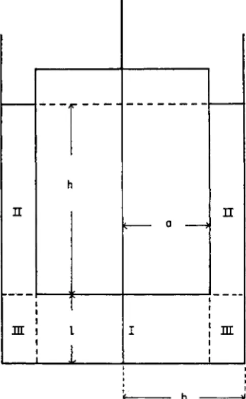
a. Theory of the End-effect for Plane Ends

We will consider first the calculation of the end-effect for the arrange-

ment shown in Fig. 5 , and subsequently, in a later section, for an arrange-

ment in which the ends of the cylinders consist of coaxial cones with com-

mon vertex.

(22)

38

^{S. OKA}

M

il

* Δ h <

Fi g . 7. End correction AH for a coaxial cylinder viscometer

We will consider here the calculation of the end-effect for the special case of a Newtonian liquid in the arrangement of Fig. 5 as mentioned in the Introduction. I t is possible to obtain an expression for AH as a function of

A, B, H, and I. However, it is not possible to obtain an expression for AH in

closed form for the general case.

²²

Let us assume without loss of generality that the outer cylinder is fixed.

The problem is to find the relation between the angular velocity Ω and the torque M. For this purpose the previous assumptions (i) to (v) are made again. These assumptions will of course hold, provided that the angular velocity Ω is sufficiently small.

In order to obtain a solution of equation (22) satisfying the appropriate boundary conditions, we imagine that the space occupied by the liquid is divided into three regions I, I I , and I I I , as in Fig. 8. Let us denote the angular velocity ω for these regions by ω

^{( 1 )},

and take co

⁽²⁾

, and Ω

^{( Ό )}⁽³⁾, respectively,

(2)

Ζ

+

^I

I

Ω + αΩ Σ

^{. . ΗΠΖ}¹^Τ^/ΗΠΝ\

(ΙΑ

²

) - (î/fe

²

) **(1/α*) - (im** Ω

+ οΩ Σ ΒΗ cosh KN(H — Ζ) Ρ

(ϋητ)

(24) ο

⁽³⁾

= οΩ Σ C

^N

sinh Uz + 1).ΊΑ^Τΐ

η=ι R

+ «Ω Σ DN sinh Κ

^Η(Ζ + I) ,

(23)

where Ιχ is a modified Bessel function of the first kind and first order, and

ρ{κ^ητ)

is given by

ρ(κ^ην) = Jx(Kⁿr)Yx(Kⁿa) — Yx(Kⁿr)Jx(Kⁿa). kⁿ

and

κ^η

are respectively the nth positive roots of the equations

Jx(kb) = 0

and

ρ(ώ) =

0 . I t may be seen that equation ( 2 4 ) satisfies equation ( 2 2 ) as well

as the boundary conditions. The nondimensional coefficients A

ⁿ

, B„ , C

ⁿ ,

and D

ⁿ

are to be determined from the conditions that the angular velocity

ω as well as the components τ^Τφ and Τφ^Ζ

of the stress tensor must be con- tinuous at both boundaries between the regions I and I I I and the regions I I and I I I . These conditions, in explicit form, are

( - l ) W t fe?) An = 2 - ± C m Jf"f/ t 1 ! ^

\ I / m = i (kj/ηπ)2 + 1

( - D W / . ( = P ) a .

Ji{kma)k^ml

sinh

2k^ml

21 ^ ^ sinh 2KJ

Σ

^Γ^{J2K^majK}^mi s i n n L\zmi ΔΙ ΤΓ< N

(kj/ηπ)2 + 1 π α m = i m (KJ/IIT)2 + 1

(Β. COSh K

nh - Ζ )^Λ

Sinh ,ηΟ ^ / ^ ^ (2δ)

, J _ , ^ Ji(k^ma) sinh fcji

fin m = l A/jn Kn

(Bn Sinh Knh + D

ⁿ

**COSh *J)**

_ _ Q J\{k^ma)k^m

cosh fc

^m

Z

m=»l

In the derivation of the above equations use was made of theorems on finite Hankel transforms.

²³

Now we proceed to calculate the torque M on the inner cylinder. This torque consists of a torque M

^x

due to the stress on the bottom surface, and a torque M

²

due to the stress on the cylindrical surface. Then

Μ χ = 2 t h;

f r

³ (^d4^)

dr,

M2 = - 2 π α %

Γ ( ^ ) dz Substituting equation ( 2 4 ) into these equations we find that

Mx = Μχ° + Μχ', M2 = M2 + M2' ,

where

2 3 S. Oka and Y . Sato, Bull. Kobayashi Inst. Phys. Research 3, 104 (1953).

(24)

40

S . O K A 4

— = \ - 1 — ( ζ ) Ι έ En cosh k α

^Δ

a L V v J

[ n - i ⁿhJ²(kⁿa)

2 b „ sinh Kⁿh

7Γ a n - l Kn& C O S h Kn(l + A) j '

where Z?

ⁿ

and F

ⁿ

are functions of the three nondimensional parameters σ,

Η, and L, while kⁿ

and κ

^Λ

have the same meaning as before.

6. V l S C O E L A S T I C L I Q U I D S20

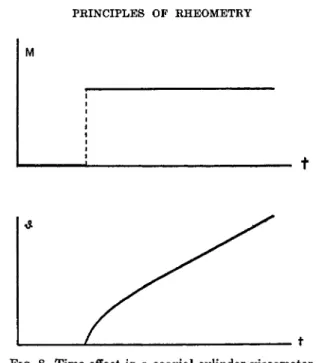
It has previously been assumed that the liquid is inelastic, that is, that the flow is steady. In practice, the average retardation of the liquid may not be vanishingly small, as it is for example in water at room temperature.

The angular displacement â of a cylinder as a function of time may be as in Fig. 8, when the torque M applied to the cylinder varies as shown.

, , 0 7Γ(Ζ

Μχ' = 2ra\ü Σ 4„7

²

-

¹ ^Κ ^Ι

' (26)

η - 1 Κη

Hence Μ may be written

²⁴

in the form of equation (23) with

**τ-*?[>-6)1 HîS^Ct)**

^{( 2 7}⁾

. 8 ! f

^D

sinh K

ⁿh\

+ - - 2 ^ # n

—- f ,

7Γ α n - l ΚΛΛ

J

where the first term in the braces corresponds to the end correction due to the bottom of the inner cylinder without the edge-effect, the second term to the edge-effect, and the third term to the effects of both the end and the free surface. Since the coefficients A

n, andßⁿ

are functions of nondimen- sional parameters

σ

= a/b, H = A/6, L = l/b,

then Ah/a is also a function of these three nondimensional parameters σ.

Η, and L.

A formal solution of the problem of the end-effect has been previously obtained by a different procedure.

²²

The result is

24 S. Oka,

Bull. Kobayashi Inst. Phys. Research

^7, 13 (1957).

(25)

FIG. 8. Time-effect in a coaxial cylinder viscometer

If we consider only times which are long compared to the average retarda- tion time, then & is constant and is taken equal to Ω. Thus the non-New- tonian flow behavior of elastic liquids may be analyzed in the same way as for the hypothetical inelastic liquid.

A material manifesting linear viscoelastic behavior in shear may be speci- fied by either of the equations:

y(t) = / rit) =

I

1

dr(u) du

1