Geoinformatics
Prof. Tamás, János
Fórián, Tünde
Geoinformatics:
Prof. Tamás, János Fórián, Tünde Publication date 2011
Szerzői jog © 2011 Debreceni Egyetem. Agrár- és Gazdálkodástudományok Centruma
Tartalom
... v
1. Introduction ... 1
1. ... 1
2. 1. Base components of GIS ... 1
2.1. 1.1. Vector data ... 2
2.2. 1.2. Raster data ... 3
2.3. 1.3. Geospatial innovation ... 5
2. 2. Geographic and projected coordinate system ... 7
1. ... 7
1.1. Practice 1: Define coordinate system in ArcGIS ... 9
1.1.1. Exercise 1.1. ... 9
1.1.2. Exercise 1.2. ... 10
1.2. Practice 2: Rectify an image map to EOV coordinate system in ArcGIS ... 12
1.2.1. Exercise 2.1. ... 13
1.2.2. Exercise 2.2. ... 16
3. 3. Surface modelling ... 19
1. ... 19
2. 3.1. TIN model ... 22
3. 3.2. DEM – DTM - DSM ... 24
4. 3.3. New technologies in surface modeling ... 26
5. 3.4. Surface or spatial analysis tools ... 29
5.1. Practice 3: Create digital surface models from vector data ... 31
5.1.1. Exercise 3.1. Create TIN surface features in ArcGIS ... 31
5.1.2. Exercise 3.2. Delineate TIN Data ... 33
5.2. Practice 4: Spatial analysis tools ... 35
5.2.1. Exercise 4.1. Create a DEM with ArcGIS ... 35
5.2.2. Exercise 4.2. Create slope maps from DEM raster ... 36
5.2.3. Exercise 4.3. Display 3D view ... 37
4. 4. Remote sensing ... 39
1. ... 39
2. 4.1. Sensors ... 41
3. 4.2. Multispectral ... 44
4. 4.3. Hyperspectral ... 47
4.1. Practice 5: Represent spectral profile of an hyperspectral image ... 48
4.1.1. Exercise 5.1. Display hyperspectral image- true color ... 49
4.1.2. Exercise 5.2. Display hyperspectral image (RGB) ... 51
4.1.3. Exercise 5.3. Create spectral profiles ... 53
4.2. Practice 6: Representing of vegetation distribution from hyperspectral data ... 55
4.2.1. Exercise 6.1. Calculation vegetation index - NDVI ... 55
4.2.2. Exercise 6.2. Export data to ArcMap ... 58
5. 5. Agricultural application of remote sensing data ... 60
1. ... 60
1.1. Practice 7: Create spectral scatter plot ... 70
1.1.1. Exercise 7.1. 2D Scatter Plots interactive classification ... 70
1.1.2. Exercise 7.2. Creation of ROI ... 73
1.2. Practice 8: Classification methods ... 75
1.2.1. Exercise 8.1. n-D Visualizer ... 75
1.2.2. Exercise 8.2. Spectral Angle Mapper Classification ... 77
6. 6. Land use – land cover modelling ... 81
1. ... 81
1.1. Practice 9: Land cover change examination ... 94
1.1.1. Exercise 9.1. Land cover map ... 95
1.1.2. Exercise 9.2. The evaluation of gains, losses and net change ... 97
7. 7. Environmental modelling ... 101
1. ... 101
2.1. Practice 10: Environmental impact assessment ... 109
2.1.1. Exercise 10.1.: The examination of the building of factories project ... 109
8. 8. Decision Support System (DSS) ... 117
1. ... 117
9. References ... 121
1. ... 121
2. Manuals, Tutorials ... 124
10. Appendix ... 125
1. ... 125
A tananyag a TÁMOP-4.1.2-08/1/A-2009-0032 pályázat keretében készült el.
A projekt az Európai Unió támogatásával, az Európai Regionális Fejlesztési Alap társfinanszírozásával valósult meg.
1. fejezet - Introduction
1.
This curriculum presents the components of the geographical information systems, disciplines, as well as primary and secondary data collection procedures. The Geographic Information System (GIS) technology is one of the most important examination methods for decision support to solve of the global or local environmental problems. Therefore the GIS technology is applied widely in education. The students learn the elements of cartographical experience, and the importance of the projection systems in GIS. It introduces the vector or raster models; and details methods of geoinformatical database construction, the bases of the display and image interpretation, and the applicable commands and tools in GIS. In this curriculum the types of the digital elevation models, the relation between the global positioning system and geoinformatical applications are explored. This book demonstrates the possibility of application of GIS, and the geoinformatical decision support. The curriculum investigates the practical problems of the national or international geoinformatical projects through case studies.
The practices of this curriculum was worked out for practical purposes used by some of the most popular GIS software‘s manuals and tutorial guides (ArcGIS™, ERDAS Imagine™, ENVI™).
2. 1. Base components of GIS
The Geographic Information System (GIS) is a method or science, which involves data collecting and storing and interpreting; the spatial relationships between objects, phenomena, geographic entities or information;
spatial analysis and modelling. It commonly could be also called Spatial Information System (SIS). GIS data is a digital representation of objects or phenomena that take place on or below the surface. It could provide different parameters of objects such as area, temperature, high, elevation; and categorize based on attributes.
The georeferenced data may be presented in table, map or several image forms. Consequently the GIS could provide answers to questions regarding spatial or geographical information.
The first software for the management and manipulation of geographic data, the Geographical Information System (GIS) appeared in the computer market in the mid-1960s. The widespread rapid diffusion of GIS starting in the 1990s has enormously increased retrieval, elaboration and analysis capabilities of available data stored in the archives of public administrations, agencies and research institutes that are fundamental for studying and planning the real world. (Gomarasca, 2009)
Nowadays there are a lot of kinds of special GIS software, which operate in similar way, but create different file types. The users need wide practice knowledge to process geoinformatical problems. The GIS database can be applied in numerous areas of sciences – for examples: geographical, economical, social, industrial – to planning, modelling and decision support.
The GIS stores two types of data that are combined on a map. However the software packages use not same logic and file types to archive or store this data. The geoinformatical technique use vector and raster layers. To create map or perform analysis users work with both type of data simultaneously.
Every GIS file or project can be joined with a metadata file. A metadata record is a file of information, which captures the basic characteristics of a data or information resource. It represents who, what, when, where, why, and how of the resource. It describes the content, quality, conditions, location, author, and other characteristics of data. Several metadata creation tools and metadata style sheets are available from within various geospatial software packages such as ArcGIS™, AutoDesk™, ERDAS™, and Intergraph™. (Shekhar and Xiong, 2008)
2.1. 1.1. Vector data
One vector layer represents geographic entities like vector data, as geometric shapes, or feature classes depending on softwares. A vector map involves point (such as sampling point, tree, monitoring well), line (such as road, railway, electric wire) or polygon (such as forest path, census track, lake, soil patterns) features, which represent discrete objects, spread of phenomenon, or natural elements. Every feature is encoded with X and Y coordinate pairs or as a series of coordinate pairs in a specified projection, and attributes. The attributes can be any special information, such as address, name, value, and datum; and stored with a traditional database management software program.
Introduction
The quality of vector data representation of images is supposed to be better than using the traditional bitmap.
The quality of vector data does not degrade with scaling, which makes it a better choice for images such as logos, which are resized frequently (Shekhar and Xiong, 2008).
2.2. 1.2. Raster data
This type of digital data represents geographic entities as cell values – rasters. One raster layer can represent only one type of information, for example: elevation, soil type, nutrition content, vegetation type. A raster image is divided into grid cells in which the qualitative or quantitative values can be recorded. This value has to be numeric value. While a raster cell stores a single value, it can be extended by using raster bands to represent red, green and blue (RGB) colours, or an extended attribute table with one row for each unique cell value (Shekhar and Xiong, 2008). Cell values can also be derived or calculated values, such as slope, aspect, distance or probability.
The size chosen for a raster cell of a study area depends on the data resolution required for the most detailed analysis (Fig. 1.5.). The extent of one pixel can be m2, km2, or Sq In depending on the type of the projection.
The size of the cell must be small enough to capture the required detail, but large enough so that computer storage and analysis can be performed efficiently (Shekhar and Xiong, 2008).
Introduction
On the first video you can see the vector layers on the study area and the labelling process in ArcView 3.3 environment. The layers and the attribute tables are opened arrow, and the lists of the descriptive attributes are listed by Identify tool.
2.3. 1.3. Geospatial innovation
While there is a growing apprecia¬tion for cross-over applications enhanced with raster and vector analysis tools, the industry's current desktop and server-based offerings largely remain segmented. Disconnected GIS, CAD, engineering, photogrammetry, and remote sensing solutions only partially address the need for creating, maintaining, sharing, and using geospatial data to understand an event for a given location. Geospatial software users are discon¬nected from key data and other users when using their analytical tools. While server-based technologies have existed for years, the majority of users still operate in the desktop environment. Ironically, these same users are likely to be well-connected to the world through instant messenger, Linkedln, Facebook, Twitter, and other social networks. (Stojic, M. and Sims, J. 2011) According to Stojic, M. and Sims, J. (2011) the geospatial information life cycle serves as the pipe connecting the engines. Geospatial data is fuel, which, when sparked by change on the earth's surface, drives the Dynamic GIS to exploit the wealth of content in the 5D Information Cloud.
The four engines that power the lnformation Cloud are capture, process, share, and deliver. The geospatial information life cycle serves as the pipe connecting the engines. Geospatial data is fuel, which, when sparked by change on the earth's surface, drives the Dynamic GIS to exploit the wealth of content in the 5D Informa¬tion Cloud.
The first engine includes airborne sensors (airborne digital imaging, LiDAR, UAV), satellites, and terrestrial sensors (total station, GPS, video, terrestrial LiDAR, handheld devices). With all these sources feeding the Information Cloud, the combined data and metadata are the fuel that is fed through the geospatial information life cycle into the second engine for data fusion, processing, and production.
The second engine includes the geospatial processing tools for fusing and integrating geospatial source content into software applications for the creation and update of geospatial data and informa¬tion products.
The third engine powering the Information Cloud is the ability to manage, fuse, and share geospatial data across departments and regions, connecting to an organization's hub of geospatial data and information. With increasing change, data volumes expand and the data captured and processed from a wide variety of "sensing"
sources creates a data management problem for finding and using geospatial data throughout an organization.
By effectively managing all sources of geospatial data (including GIS, CAD, surveying, remote sensing, and photogrammetry), the value and usability of that data increases beyond departmental compartments and across spatial domains to users who have a need to understand the changing earth.
The fourth engine for fully lever¬aging the Information Cloud enables the delivery of geospatial data AND dynamic information products. This is done through on-demand geoprocessing over the Internet, to mobile clients and the cloud through vertical market-focused SaaS implementations. The delivery engine leverages stand-ards-based spatial data infrastructure (SDI) concepts, high-performance technologies, and geoprocessing Web services for delivering geospatial information to Web portals, mobile clients, and a variety of thin- and smart-client applications.
The Dynamic GIS catapults our entire industry into a new era, where integrated geospatial systems replace the traditional domains of GIS, remote sensing, photo¬grammetry, surveying, and mapping. (Stojic, M. and Sims, J.
2011)
2. fejezet - 2. Geographic and projected coordinate system
1.
All spatial data file in GIS are georeferenced. Describing the correct location of features requires a framework for defining real-world location. This process, and the assigning map coordinates to the image data is called georeferencing. Georeferencing allows combining dataset representing information about the same location.
(ArcGis 9 User Manual 2006) Georeferencing information includes coordinate information. Dataset are stored using coordinates, which describe the correct position of the features. This information pair is very important to use a GIS analysis or to measure on the vector or raster map composition.
The geographic coordinate system describes the geographic location on the Earth‘s surface with Northern, or Southern latitude (from 0º to 90º) and Eastern, or Western longitude (from 0º to 180º) degrees. It is a spherical coordinate system composed of parallels of latitude (Lat) and meridians of longitude (Lon). The unit of geographic coordinate system is the degree.
The projected coordinate system helps to transform the features to a flat plane with the transformation formula.
The projected coordinate system use two axes: x – axis (horizontal, east-west direction); y-axis (vertical, north- south direction). The unit of projected coordinate system is the feet or meter. The geodetic reference system, datum, is constituted by fixing the following elements: ellipsoid, point of emanation, azimuth.
To define a special reference ellipsoid user has to select a geodesy datum, which is established by national or international geodetic surveyors. Most datum only attempt to describe a limited part of the earth, so these are called local datum. However there are some geodetic systems describing entire earth‘s surface, such as World Geodetic System (WGS84). WGS84 system is used for positioning through GPS (Global Positioning System) technology.
The spatial reference of a point is given by a triple of Cartesian coordinates (X, Y, Z) referred to a system having its origin in the centre of the ellipsoid. An example of Cartesian geocentric coordinates is the WGS84 reference system in which the Cartesian triple are XWGS84, YWGS84, ZWGS84 (Gomarasca, 2009).
2. Geographic and projected coordinate system
the list of the supported map projections is different, but every program packages process many standard coordinate systems and numerous local system. The ArcGIS versions support the Hungarian coordinate system (EOV) so called HD1972 Egységes Országos Vetület. As well as user can also create a custom coordinate system with describing the projection file.
1.1. Practice 1: Define coordinate system in ArcGIS
1.1.1. Exercise 1.1.
If the input dataset or vector layers, created by GPS survey or rectified in any software ambient, possess any associated projection parameters, but the coordinate system has not defined in ArcGIS first the projection file has to be defined before any analysis.
1.Start ArcMap, with a new, empty map, and add the data downloaded from GPS with parameters of the known coordinate system. The data must not have a defined coordinate system.
2.Open the ArcToolbox Window with Toolbox icon. Open the „Data Management Tools / Projection and Transformations / Define Projection module.
3.Select the dataset or layer.
4.Click the Coordinate System tab, and choose the Select tab. Navigate to the WGS84 coordinate system in the Projection Coordinate Systems folders. OK
To assign the coordinate system, ―import‖ button can be useable, if there is any layer with required coordinate system in the database. To create new custom coordinate system ―new‖ button has to be used.
When the coordinate system is defined, the other data, which add to the ArcMap session, is fitting into the current coordinate system.
5. Add a new data layer with other coordinate system to the map composition.
One dialog box appears to show which geodetic datum of map layers differ from the other maps.
2. Geographic and projected coordinate system
The geodetic datum of the layer can be defined in ArcCatalog. In the catalogue tree, navigate and select the layer.
Right-click on the layer name and click Properties. On the Properties dialog box, assign coordinate system according to previous method.
If you need to change the coordinate system of any layer to a different one, Project (feature layer) or Project Raster (raster layer) tools has to be used.
7. Open Data management Tools / Projection and Transformation / Feature / Project tool – in the case of vector layer; or Data management Tools / Projection and Transformation / Raster / Project raster tool – in the case of raster layer.
8. Enter the input and output layer name.
9. Select the required coordinate system.
10. Select the transformation method. OK.
1.2. Practice 2: Rectify an image map to EOV coordinate system in ArcGIS
This process involves identifying a series of ground control points (GCPs) with known the real location - x,y coordinates. There are many different types of GCPs that can be used to identify locations, such as road or stream intersections, street corners, or the corners of the buildings. The control points are used to convert the raster dataset to the spatially correct location. The connection between one control point on the raster dataset and the corresponding control point on the aligned target data is a link. The number of links depends on the transformation method to project the raster dataset to map coordinates.
Conflation technologies are applied in many application domains using high quality spatial data such as GIS. In general, the goal of conflation is to combine the best quality elements of both datasets to overlay different
2. Geographic and projected coordinate system
These exercises were worked out for practical purposes used by ArcGIS® 9 Using ArcGIS Desktop.
1.2.1. Exercise 2.1.
Conflation method with ArcGis software
1. In ArcMap, display the layers having map coordinates.
2. Add the raster dataset that you want to georeference.
3. Open the Georeferencing toolbar under View menu, point to Toolbars, and click Georeferencing
4. In the table of contents, right-click the referenced dataset and click Zoom to Layer.
5. From the Georeferencing toolbar, click the Layer drop-down arrow and click the target raster layer that you want to georeference.
6. Click Georeferencing and click Fit To Display.
7. The target layer will display with the raster dataset in the same area. If both layers are raster images, the target layer has to be transparent. Open the Effects toolbar under View menu, point to Toolbars, and click Effects.
8. Click the Layer drop-down arrow, select the target raster layer and use the Adjust transparency icon to change the visibility of the layer.
9. Look for GCPs such as road intersections, land features, building corners or other objects that you can identify and match in your raster dataset and aligned datasets. Before placement of the GCPs, switch off the Auto adjust tool under the Georeferencing menu in order to prevent the target raster from becoming deformed.
2. Geographic and projected coordinate system
11. Add enough links for the type of transformation. You need a minimum of three links for a spline or 1st-order polynomial (affine), six links for a 2nd-order polynomial, and ten links for an affine or 3rd-order polynomial.
12. Click View Link Table to evaluate the transformation. Select the transformation method from drop-down list and examine the residual error for each link and total RMS error. All error values are expressed in term of the root mean square error (RMSE), it is an estimator of general model performance - precision (Zeilhofer et al., 2011). The (RMS) average value of each residual gradient grid is calculated in order to give an estimate of the error in the numerical gradient values at each cell size (Jones K. H., 1998).
You can delete an unwanted link from the Link Table dialog box. After deleting incorrect GCP, use Auto adjust to verify the changes.
13. If you‘re satisfied with the registration, click Georeferencing menu and select Update Georeferencing to save the transformation information with the raster dataset. This creates a new file with the same name as the raster dataset but with an .aux.xml file extension.
14. You can permanently transform your raster dataset after georeferencing by using the Rectify command;
click Georeferencing and click Rectify
This exercise was worked out for practical purposes used by ArcGIS® 9 Using ArcGIS Desktop.
1.2.2. Exercise 2.2.
Conflation method with ERDAS software
The above mentioned process can be performed in other software environment also; however there are some differences from the method in ArcGis. In this exercise, you rectify a previous soil map using a georeferenced topographic map of the same area. The topographic map is rectified to the Hungarian coordinate system – EOV projection, however this projection is not defined in Erdas.
1. Start the Erdas Imagine software.
2. Click the Viewer icon on the ERDAS IMAGINE icon panel to open two Classic Viewer windows. Then select the target raster layer in the first viewer and the referenced raster in the second viewer. The Erdas software works with numerous raster file format as compared with the ArcGis.
The first difference is the display, since the images is opened in two independent windows. When the topographical map is opened, the coordinate values are shown in the status bar.
3. Start the Raster menu / Geometric Correction Tool from the first Viewer (the Viewer displaying the file to be rectified).
2. Geographic and projected coordinate system
4. The Set Geometric Model dialog opens. In the Set Geometric Model dialog, select Polynomial and then click OK. The Geo Correction Tools open, along with the Polynomial Model Properties dialog. Choose the appropriate polynomial order and the map units to meter.
Use the Add / Change Projection button to select appropriate projection if the projection system is defined by Erdas. However the Hungarian EOV coordinate system is not specified in Erdas software, consequently the projection type remains Unknown. You can also create custom projection file in Erdas, but this curriculum doesn‘t mention this topic.
5. Click Close in the Polynomial Model Properties dialog to close it for now. You can also select these parameters later with using the icon in the Geo Correction Tools.
6. The GCP Tool Reference Setup dialog opens. Select the default of Existing Viewer in the GCP Tool Reference Setup dialog by clicking OK. However you can choose Keyboard Only option, if you know the coordinates of the ground control points.
7. The GCP Tool Reference Setup dialog closes and a Viewer Selection Instructions box opens, directing you to click in a Viewer to select for reference coordinates.
8. The Chip Extraction Viewers (Viewers #3 and #4), link boxes, and the GCP Tool open. The link boxes and GCP Tool are automatically arranged on the screen (you can turn off this option in the ERDAS IMAGINE Preferences). You may want to resize and move the link boxes so that they are easier to see.
9. In the first Viewer, select one of the known control point. Click the Create GCP icon in the GCP Tool, and point with mouse on the target raster data to place on control point, then point the raster dataset with coordinate system to place on the associated control point.
In order to see easier the GCPs you can change the colour under the Color columns with left click. Digitize at least two more GCPs pairs in each Viewer by repeating the above steps. The GCPs you digitize should be spread out across the image to form a large triangle. After you digitize the fourth GCP in the first Viewer, note that the GCP is automatically matched in the second Viewer, if the Toggle Fully Automatic GCP Editor icon is on.
10. Examine the residual values and the total RMS error. Select to incorrect GCPs and move to the correct place with the help of the small viewers 3-4, or delete it. To delete a GCP, select the GCP in the Cell Array in the GCP Tool and then right-hold in the Point # column to select Delete Selection.
11. Click the Resample icon in the Geo Correction Tools. The Resample dialog opens. Resampling is the process of calculating the file values for the rectified image and creating the new file. All of the raster data layers in the source file are resampled. The output image has as many layers as the input image. ERDAS IMAGINE provides these widely-known resampling algorithms: Nearest Neighbour, Bilinear Interpolation,
3. fejezet - 3. Surface modelling
1.
Nowadays the GIS models use numerous applications to evaluate or calculate the effect of the environmental phenomenon. However the modelling of the natural, hydrological, erosion process needs digital surface data, which is generated in general from vector databases (contour lines, elevation points). Consequently, the creating of surface model is fundamental in numerous area of science.
The most spectacular application of the DEMs is the representations of volcanoes, hilly or coastal region.
Geographers and geologists have developed or integrated various spatial data analysis for managing and analyzing multi-disciplinary, lithology, volcanological information or the data-sets of the anthropogenic structures (Gogu et al. 2006; Fornaciai et al., 2010; De Rienzo et al. 2008).
3. Surface modelling
DEM creation is also very important in area of the agriculture and the soils science. Casalí et al. (2009) determined the long-term erosion rates, and the remained soil surface level in vineyards with the help of the DEMs.
Furthermore, Katsianis et al., (2008) represent a formal data model and complete digital workflow in 3D using the prehistoric site in Greece, as a case study. They chosen Esri‘s ArcGIS as the unifying software platform for several key reasons: being an industry standard, incorporating a functional 3D viewing environment (ArcScene), presenting abilities for customization, having a spatial database system with object-oriented characteristics and supporting communication with external programs (Rock-Ware, EVS, CAD, Sketch Up).
The monitoring and modelling of the gully erosion was examined by Marzolff and Poesen (2009) with using a hybrid method combining stereo matching for mass-point extraction with manual 3D editing and digitizing, high-resolution DEMs.
The digital surface model is a representation of features, either real or hypothetical, in three-dimensional space.
In the last decades researchers have investigated a variety of technical issues related to 3D data processing, visualization, data management and spatial analysis in order to represent the world more or less closely to reality. A 3D surface is usually derived, or calculated, using specially designed algorithms that sample point, line or polygon data and convert them into a digital 3D surface (http://webhelp.esri.com). GIS softwares can create and store different types of surface model: TIN, raster, terrain and voxel based.
Surfer is a grid-based mapping program that interpolates irregularly spaced XYZ data into a regularly spaced grid. The grid is used to produce different types of maps including contour, vector, image, shaded relief, 3D
2. 3.1. TIN model
TINs (Triangulated Irregular Networks) are a vector data structure that partitions geographic space into contiguous, non-overlapping triangles. A TIN is a complete planar graph that maintains topological relationships between its constituent elements: nodes, edges, and triangles. The vertices of each triangle are sample data points with x-, y-, and z-values (used to represent elevations). These sample points are connected by lines to form Delaunay triangles. (Shekhar and Xiong, 2008)
3. Surface modelling
As the triangles may have variable size and shape, this structure allows a faithful representation of the Earth‘s surface, even when strong and abrupt discontinuities are present. Flat zones, in fact, can be represented from a limited number of points and described through big-sized triangular facets. The main limitation of TIN is its difficulty to be managed, having topological relations that must be explicitly declared, that are calculated and recorded on purpose; moreover triangulation algorithms are very complex. To generate a TIN, the most largely used interpolation algorithm is the above mentioned Delaunay triangulation, which provides a univocal association between the measured points and a set of polygons, called Thiessen polygons. The generated triangles are different in shape and size representing the described surface by joining the internal points of adjacent polygons. In the new structure, each point becomes a vertex of a triangle, satisfying the Delaunay criterion stating that no vertex is present within the circle circumscribed to a triangle. (Gomarasca, 2009)
The result is a triangular tessellation of the entire area that falls within the outer boundary of the data points (known as the convex hull). The Delaunay triangulation process is most commonly used in TIN modeling. A Delaunay triangulation is defined by three criteria: 1) a circle passing through the three points of any triangle (i.e., its circumcircle) does not contain any other data point in its interior, 2) no triangles overlap, and 3) there are no gaps in the triangulated surface. If iso-line data are used as input to TIN generation, both the non- constrained and constrained options are available and a better TIN result can be expected. This process ensures that triangle edges do not cross iso-lines, and the resulting TIN model is consistent with the original iso-line data. Not all triangles will necessarily meet the Delaunay criteria when the constrained triangulation is used.
(Tamás et al., 2004)
3. 3.2. DEM – DTM - DSM
The spatial topographic computerized databases or model are Digital Elevation Models – DEMs, sometimes referred to as DTMs - Digital Terrain Models. The most common method of acquiring elevation data in digital raster format is digitizing contours from a topographic map and applying an interpolation method to transform the contour data into a DEM. It is often desirable that the DEM to be used in a GIS be defined on a uniform grid even though the source data might be in a very different format - contour lines, or elevation points (Lyon J.G., 2005). Common raster DEM databases usually store data in several meters pixel resolution having vertical accuracy around several meters. The intensity values of pixels represent the height above the sea level. The smoothness of the generated DEM is highly dependent on the local interpolation methods such as neighbourhood, inverse weighted distance, or kriging. The one of the most important operation related to DEM accuracy is interpolation method.
Point interpolation is normally used to estimate unknown values from a sample of an attribute that varies continuously over space. Areal interpolation is used to reaggregate entity data into a different areal partition of space. Although the two types of spatial interpolation solve very different geographic problems, point interpolators can also be used to reaggregating data under certain conditions as described below. (Lin et al., 2011)
3. Surface modelling
Digital Terrain Models (DTMs) are getting more and more important in geographical data processing and analysis: they allow modelling, analysis and visualization of phenomena related to the territory morphology (or to any other characteristic of the territory different from elevation) (Gomarasca, 2009). There is one more definition related to surface model, the Digital Surface Models (DSM). DSM describes the terrestrial surface, including the objects covering it like buildings, vegetation and in general describes it through known geometric primitives (rectangles or triangles). 3D geoinformation research is often related to the representation of the built or mane-made environment (Kjems et al, 2009).
4. 3.3. New technologies in surface modeling
A terrain dataset is a TIN-based data structure with multiple levels of resolution. Terrains include pyramids that provide the appropriate levels of detail for use at multiple scales. A terrain dataset is built from multiple data sources such as LIDAR mass point collections, 3D break lines, and 3D-based survey observations. The data sources used to create terrain datasets are managed as a set of integrated feature classes in the geodatabase.
(http://webhelp.esri.com)
The laser technology is now available for photogrammetric. The technology is a still developing and continuous representation method of the Earth‘s surface. It produces a huge amount of data to be processed, visualized and integrated into the photogrammetric process.
Laser scanning is a surveying technology for rapid and detailed acquisition of a surface in terms of a set of points on that surface, a so-called point cloud. Laser scanners are operated from airborne platforms as well as from terrestrial platforms (usually tripods). The time elapsed between emitting and receiving a pulse is multiplied by the speed of light to derive the distance between the laser range finder and the reflecting object.
This distance is combined with position and attitude information of the airborne platform, as well as the pointing direction of the laser beam, to calculate the location of the reflecting object. (Shekhar and Xiong, 2008)
3. Surface modelling
During last years the LIDAR (Light Detection And Ranging) has been used as a very good option to terrestrial surface surveying. In recent years, LIDAR sensors have been widely used to measure environmental parameters such as the structural characteristics of surface, features, or forests. This new data acquisition technology is now capable of collecting data in a much denser and more precise manner. For example, LiDAR technology, which have dispersal and irregular data structure, can acquire up to 16 points per 1m2 with position accuracy around 0.1m (Dalyot and Doytsher, 2009). It can survey 3D positions over the terrestrial surface at speed beyond comparison to the Topography or Photogrammetry (De Lara et al., 2009).
LIDAR provides a 3D cloud of points, which is easily visualized with Computer Aided Design software. Three- dimensional, high density data are uniquely valuable for the qualitative and quantitative study of the geometric parameters of plants. LIDAR allows fast, non-destructive measurement of the 3D structure of vegetation (geometry, size, height, cross-section, etc.). Results are demonstrated in fruit and citrus orchards and vineyards, leading to the conclusion that the LIDAR system is able to measure the geometric characteristics of plants with sufficient precision for most agriculture applications. (Rosell et al., 2009)
Moreover the high-resolution LIDAR DSM data is able to quantify three-dimensional buildings (Lohani and Singh 2008; Chio 2008), urban morphology and its impacts on the spatio-temporal variability of solar radiation (Yu et al. 2009).
3. Surface modelling
Many researchers propose 3D grid representation (voxels) as the most appropriate data format to visualize continuous phenomena in true 3D format. A voxel (volumetric pixel or Volumetric Picture Element) is a volume element, representing a value on a regular grid in real three dimensional space. (De Rienzo et al., 2008;
Kirkpatrick and Weishampel, 2005; Dong, 2009)
5. 3.4. Surface or spatial analysis tools
The surface model of the topographic surface can be used to characterizing geomorphological features over the different applications, such as slope, aspect, length of the slope, curvature, perspective views, view shed analysis, height profiles and volume calculations. This family of tools is generally calculated from the finest spatial scale database.
Slope maps are also raster datasets where the cell value represents the angle between the horizontal and the local gradient of the DEM. There are special classes of slopes depending on the different area of science.
The cell values of aspect maps represent the angle (azimuth) between the north direction and the local gradient (planar components). Usually nine classes are considered: one referred to the null value (flat areas), the other height to the main direction sectors (north, northeast, east, south-east, south, south-west, west, north-west).
3. Surface modelling
The Hillshade tool creates a shaded relief raster from a raster. The illumination source is considered at infinity.
The hillshade raster has an integer value range of 0 to 255.
Performs visibility analysis on a raster by determining how many observation points can be seen from each cell location of the input raster or which cell locations can be seen by each observation point. The visibility of each cell centre is determined by comparing the altitude angle to the cell centre with the altitude angle to the local horizon. The local horizon is computed by considering the intervening terrain between the point of observation and the current cell centre. If the point lies above the local horizon, it is considered visible.
(http://webhelp.esri.com)
5.1. Practice 3: Create digital surface models from vector data
5.1.1. Exercise 3.1. Create TIN surface features in ArcGIS
1.Start ArcMap, with a new, empty map
2.Open the input vector layers (contour or elevation point). The data must have a defined coordinate system (see above) with X and Y coordinates, and Z – elevation values. Height (Z) Field is the name of the attribute to be used for height information.
3.Under the Tools menu / Extensions, select the 3D Analyst option.
4.First one TIN must be defined using the Create Tin function. Open the ArcToolbox Window with icon. Select the 3D Analyst toolbox / TIN Creation tools / Create TIN tool. Enter the output file name and its path.
5.Select the 3D Analyst toolbox / TIN Creation tools / Edit TIN tool. Select the input TIN. Add features to the existing TIN. Multiple feature layers can be added at the same time with the + icon. From the drop-down list select the height field - Z. OK.
3. Surface modelling
6.Click the name of the TIN in Table of Content window, choose the Properties option. In the Properties window select the Symbology tab. Add a new Renderer (Face elevation with graduated color ramp) to Legend.
Choose appropriate color ramp, and define the number of classes. Apply.
5.1.2. Exercise 3.2. Delineate TIN Data
Turn of the contour layer to examine the TIN, where exists ―false‖ value at the edge of the area (too length side of the triangles).
7.Select the 3D Analyst toolbox / TIN Creation tools / Delineate TIN Data Area tool to define the data area, or interpolation zone, of a TIN based on triangle edge length. Define the value of the Maximum Edge Length.
8. Turn on the input vector layer to examine the result.
3. Surface modelling
5.2. Practice 4: Spatial analysis tools
5.2.1. Exercise 4.1. Create a DEM with ArcGIS
Use the previous input vector data having coordinate system (X and Y coordinates) and Z – elevation values to create DEM.
1.Open the ArcToolbox Window with icon. Select the 3D Analyst toolbox / Raster interpolation / Topo to raster tool.
2.Multiple feature layers can be added at the same time with the + icon. From the drop-down list select the height field – Z, and type of the input data – contour or point. The default output file is a temporally file. Enter the output file name and its path. Define the cell size of the output raster. OK.
3.Click the name of the raster DEM in Table of Content window, choose the Properties option. In the Properties window select the Symbology tab. Choose appropriate color ramp, and define the number of classes. Apply.
5.2.2. Exercise 4.2. Create slope maps from DEM raster
4.Select the 3D Analyst toolbox / Raster surface tools / Slope tool. Click the Input surface dropdown arrow and click the surface for which you want to calculate the slope. The output measurement units for slope can be in degrees or percentages. So choose the Output measurement units. Change the default Output cell size. Specify a name for the output, or leave the default to create a temporary dataset in your working directory.
3. Surface modelling
6. Click the Method drop-down arrow and click the classification method you want to use. Click the Classes drop-down arrow and click the number of classes you want to display. Type a new upper value of the range on the basis of histogram or specific intervals. OK. Enter Label for every class. OK.
5.2.3. Exercise 4.3. Display 3D view
7.Start the ArcScene from the ArcMap with the icon. Add the raster layers – DEM, slope - to Table of Content.
8.First set the base height of DEM. Double click on the layer name. Click the Base Height tab. Select and enter the name and path of the DEM. Set the z-unit conversion to 10, if the sample area is lowland. Examine the result.
9.Perform the previous step on the drapping layer – slope at the same way. Select and enter the name and path of the DEM. Select the Symbology tab. Choose color ramp. Select the Use Hillshade Effect option. OK.
10.Open the Effects toolbar under View menu, point to Toolbars, and click 3D Effects.
11.Click the Layer drop-down arrow; select the target raster layer – slope, and use the Adjust transparency icon to change the visibility of the layer.
4. fejezet - 4. Remote sensing
1.
Aerial photography and satellite imagery, both photographic and telemetric, recorded at various wavelengths or bands of the electromagnetic spectrum are included in these tools (Pavlopoulos et al., 2009). From classical geography, scientific activities in Earth Observation have undergone a rapid expansion, and more and more economic sectors tend to employ territorial data acquired by ground survey, global satellite positioning systems, traditional and digital photogrammetry, multi- and hyperspectral remote sensing from airplane and satellite, with images both passive optical and active microwave (radar) at different geometric, spectral, radiometric and temporal resolutions, although there is still only limited awareness of how to use all the available potential correctly.
The first photographs of the Earth taken from space were released in the early 1960s. In 1972 the U.S.A.
launched its first Earth Resources Technology Satellite ERTS-1, which was later renamed LANDSAT-1.
(Cracknell and Hayes, 1993)
The resulting data and information are represented in digital and numerical layers managed in Geographical Information Systems and Decision Support Systems, often based on the development of Expert Systems.
(Gomarasca, 2009) Remote sensing is the science and art of obtaining information about the properties of electromagnetic waves emitted, reflected or diffracted without touching the object (Campbell, 2002). Remote sensing enables a unique perspective to map and monitor on large areas because it measures emitted or reflected energy at wavelengths with a wider range than human vision.
Remote sensing includes techniques to derive information from a site at a known distance from the sensor.
Imaging data are either gathered as photographs and optically digitized, or are measured directly using a digital instrument on a remote sensing satellite or aircraft. Every element on the Earth reflects, absorbs and transmits part of an incident radiation to different percentages according to its structural, chemical and chromatic qualities.
Radar or satellite data can be used in GIS applications for numerous science areas: geology, archaeology, vegetation classification, crop monitoring, glaciology, oceanography, soil science, hydrology or pollution monitoring.
The one of most important parameters, which characterized the instruments, are the wavelength (or frequency), the amplitude, and the direction of the surveying. Electromagnetic radiance is the information reaching a sensor from the objects located on the Earth. For example, the problem with most widely used multispectral systems is that they only have a limited number of bands with each covering a very wide region in the spectrum (>
100nm); and within such a wide spectral region a lot of subtle information is averaged, generalized or even concealed. (Zhou, 2007).
4. Remote sensing
Every Earth‘s surface (soil-, rock-, vegetation-, water-, and building surface) and the variations of these have a unique spectral profile. However these unique spectral features of the surface varieties or vegetation species, such as reflectance peaks or absorption troughs in the spectrum, are often lost in broad-band spectral reflectance.
2. 4.1. Sensors
Change detection or monitoring methodology can be greatly facilitated by the use of digital imaging data from
and to do so at a potentially lower relative cost than fieldwork and mapping alone. In remote sensing, there are two typologies of instruments, passive and active, based on the source of incident radiation on the Earth‘s surface and on wavelength intervals. In passive remote sensing, sensors operate in wavelength intervals from ultraviolet to thermal infrared; in active systems such as radar, they operate in microwave intervals. In passive remote sensing, the source of information is scattered and/or absorbed solar and emitted thermal radiation, which allows us to study and characterize objects through their spectrally variable response. (Gomarasca, 2009)
A passive system is restricted to radiation that is emitted from the surface of the Earth or which is present in reasonable quantity in the radiation that is emitted by the Sun and then reflected from the surface of the Earth.
An active instrument is restricted to wavelength ranges in which reasonable intensities of the radiation can be generated by the remote sensing instrument on the platform on which it is operating. Active sensors operating in the visible and infrared parts of the spectrum, while not being flown on satellites, are flown on aircraft.
(Cracknell and Hayes, 1993)
Nowadays, a new generation of airborne hyperspectral imaging systems is available and applicable to map the environment. The ―hyper‖ in hyperspectral refers to the large number (>498) of measured wavelength bands.
Field and laboratory spectrometers usually measure reflectance at many narrow, closely spaced wavelength bands, so that the resulting spectra appear to be continuous curves. One of the hyperspectral sensor is AISA dual sensor system, which provides seamless hyperspectral data in the full range of 400 - 2500nm.The Eagle camera takes images in the visible and near infrared range (400- 970 nm), while Hawk operates in the middle infrared range (970-2500 nm) with 498 spectral channels. (Tamás et al, 2009)
4. Remote sensing
4. Remote sensing
The multispectral image can be used as a photo or a scientific basic database to subject to differences photo interpretation methods.
The Multispectral Scanner System (MSS) sensors were line scanning devices observing the Earth perpendicular to the orbital track. The cross-track scanning was accomplished by an oscillating mirror; six lines were scanned simultaneously in each of the four spectral bands for each mirror sweep. The forward motion of the satellite provided the along-track scan line progression. The first five Landsat carried the MSS sensor which responded to Earth-reflected sunlight in four spectral bands. Landsat 3 carried an MSS sensor with an additional band, designated band 8, that responded to thermal (heat) infrared radiation. Four years after the launch of the first Landsat satellite (then called the Earth Resources Technology Satellite, ERTS-1), a U.S. Geological Survey Professional Paper entitled, "ERTS-1 A New Window on Our Planet" was published. The publication documented how visual examination of images from a space-based vantage point could benefit disciplines such as geology, hydrology, forestry, geography, cartography, agriculture, land use planning and rangeland management. Landsat data have helped to improve our understanding of Earth. Thanks to Landsat, today we have a better understanding of things as diverse as coral reefs, tropical deforestation, and Antarctica's glaciers.
The 30 m spatial resolution and 185 km swath of Landsat imagery fills an important scientific niche because the orbit swaths are wide enough for global coverage every season of the year, yet the images are detailed enough to characterize human-scale processes such as urban growth, agricultural irrigation, and deforestation.
(http://landsat.gsfc.nasa.gov)
Multispectral remote sensing enables them to distinguish between different types of vegetation, rocks and soils;
clear and turbid water; and selected man-made materials.
However, in case of multi-spectral imagery the spectral response of a single pixel is often a mixture among several targets other sensors with high spectral resolution like Moderate Resolution Imaging Spectroradiometer - MODIS are not capable for observation of small patches because of their low spatial resolution. Furthermore, some sensors - like Landsat Thematic Mapper (TM) - have low spatial resolution.
Combining data from several different bands of a multi-spectral scanner to produce a false colour composite image for visual interpretation and analysis suffers from the restriction that the digital values of three bands only can be used as input data. Consequently, only three bands can be handled simultaneously. (Cracknell and Hayes, 1993)
4. Remote sensing
The wavelengths are approximate; exact values depend on the particular satellite's instruments:
• Blue, 450-515..520 nm, used for atmospheric and deep water imaging. Can reach within 150 feet (46 m) deep in clear water.
• Green, 515..520-590..600 nm, used for imaging of vegetation and deep water structures, up to 90 feet (27 m) in clear water.
• Red, 600..630-680..690 nm, used for imaging of man-made objects, water up to 30 feet (9.1 m) deep, soil, and vegetation.
• Near infrared, 750-900 nm, primarily for imaging of vegetation.
• Mid-infrared, 1550-1750 nm, for imaging vegetation and soil moisture content, and some forest fires.
• Mid-infrared, 2080-2350 nm, for imaging soil, moisture, geological features, silicates, clays, and fires.
• Thermal infrared, 10400-12500 nm, uses emitted radiation instead of reflected, for imaging of geological structures, thermal differences in water currents, fires, and for night studies.
• Radar and related technologies, useful for mapping terrain and for detecting various objects.(http://en.wikipedia.org/wiki/Multi-spectral_image)
4. 4.3. Hyperspectral
The recent development of hyperspectral sensors and image-data analysing software it is one of the most significant breakthroughs in remote sensing (Ritvayné et al.. 2009)
Hyperspectral sensors can capture data in contiguous, hundreds of narrow bands in the electromagnetic spectrum, so presents numerous possibilities for interpretation and analysis. The large numbers of bands provide for researchers vast quantities of information about the study area. Hyperspectral data can often capture the unique spectra or ‗spectral signature‘ of an object. This signature can be used to differentiate and identify materials on the basis of the spectral library provided by analysis softwares like ITT ENVI.
Hyperspectral remote sensing integrates imaging and spectroscopy in a single system which often includes large data sets due to the fine narrow subdivision of bands and the ―hyper‖ number of bands in the spectrum (Zhou, 2007).
Numerous publications dealt with the analysis of the hyperspectral data regarding to wide range of science area such as weed pattern analysis (Zhou, 2007; Tamás et al., 2006); acid mine drainage (Szucs et al., 2002; Yan and Bradshaw, 1995); soil plant systems for characterization of the distribution of heavy metals (Kabata-Pendias,
2001; Faheed, 2005); heavy metal distribution by mapping technologies (Nagy and Tamás, 2008), water management (Burai and Tamás, 2004) precision agricultural (Tamás et al., 2009).
A lot of sensors have been developed which can provide a near complete spectrum for each pixel using high spectral resolution. Calibrated hyperspectral data is comparable to laboratory spectra to identify ground materials at pure or mixed pixels. Sensors used for data acquisition can be installed in both airborne and land carrier units (Zhou, 2007; Ritvayné et al., 2009). While processing and evaluating information, it is also necessary to carry out ground measurements and collect reference data using conventional sampling.
After the radiometric and geometric correction, the hyperspectral n-dimensional data cube can be suitable for classification. This data cube contains all geographical and spectral data changing pixel by pixel.
4. Remote sensing
2.Specify the default temp directory for output temporary files.
4.1.1. Exercise 5.1. Display hyperspectral image- true color
3.If an input file has wavelengths for each band stored in the header and the file contains bands in the needed wavelength ranges, you can display a true color from the Available Bands List without having to designate the individual bands for red, green, and blue. ENVI displays the true-color image band in the red wavelength region (0.6-0.7 μm) in red, the band in the green region (0.5-0.6 μm) in green, and the band in the blue region (0.4-0.5 μm) in blue. If the file does not have bands in the needed wavelengths, ENVI uses the bands nearest to the wavelengths. This may produce a gray scale image if red, green, and blue are set to the same band.
4.In the Available Bands List, right-click on the filename.
5.Select Load True Color to load the image to a new display group if no display groups are open.
6.Select Load True Color to new to load the image to a new display group.
4. Remote sensing
When you display a file from the Available Bands List, a group of windows will appear on your screen allowing you to manipulate and analyze your image. This group of windows is collectively referred to as the display group. The default display group consists of the following:
• Image window: Displays the image at full resolution. If the image is large, the Image window displays the subsection of the image defined by the Scroll window Image box.
• Zoom window: Displays the subsection of the image defined by the Image window Zoom box. The resolution is at a user-defined zoom factor based on pixel replication or interpolation.
• Scroll window: Displays the full image at subsampled resolution. This window appears only when an image is larger than what ENVI can display in the Image window at full resolution.
4.1.2. Exercise 5.2. Display hyperspectral image (RGB)
8.You can open image files or other binary image files of known format. From the main menu bar, select File menu / Open Image File. When you open a file for the first time during a session, ENVI automatically places the filename, with all of its associated bands listed beneath it, into the Available Bands List. If a file contains map information as well, a map icon appears under the filename.
9.To display in RGB format, select the appropriate band to Red, Green, and Blue from the Available Bands List window, under the file name. Load RGB. This method is useful to represent the differences in the study area on basis of spectral bands.
4. Remote sensing
4.1.3. Exercise 5.3. Create spectral profiles
10.Use ENVI's Z Profiles to interactively plot the spectrum (all bands) for the pixel under the cursor. For higher spectral dimension datasets such as hyperspectral data, using a BIL or BIP file allows real-time extraction of spectra. From the Display group menu bar, select Tools / Profiles / Z Profile (Spectrum) tool.
11.In the display group, right-click and select Z Profile (Spectrum). Select a pixel in either the Image window or the Zoom window to plot the corresponding spectrum in the plot window. A vertical line (plot bar) on the plot marks the wavelength position of the currently displayed band. If a color composite image displays, three colour lines appear, one for each displayed band in the band's respective color (RGB).
4. Remote sensing
12.To plot multiple Z Profiles (spectra) over each other in the Spectral Profile plot window, select Options / Collect Spectra from the Spectral Profile plot window menu bar.
13.From the plot window menu bar, select Edit / Plot Parameters. The Plot Parameters dialog appears.
4.2. Practice 6: Representing of vegetation distribution from hyperspectral data
4.2.1. Exercise 6.1. Calculation vegetation index - NDVI
1.The NDVI (Normalized Difference Vegetation Index) values indicate the amount of green vegetation present in the pixel. Values of the NDVI index are calculated from the reflected solar radiation in the near-infrared (NIR) and red (R) wavelength bands, i.e. 580–680 nm, and 730–1100 nm, respectively. NDVI can be determined using the following formula: NDVI = (NIR – R)/(NIR + R). Higher NDVI values indicate more green vegetation. Valid results fall between -1 and +1. Before analysis define the wavelength unit of measure of the hyperspectral image.
2.Select File menu / Edit ENVI Header tool. Choose the hyperspectral image file, OK. In the Header Info window select the Edit Attribute button / Wavelength tool. In the next dialog window select the units of wavelength - Nano or micrometer depending on the hyperspectral imagery method.
3.From the ENVI main menu bar, select Spectral menu / Vegetation Analysis / Vegetation Index Calculator tool.
The Input File dialog appears.
4.Specify the Input File Type from the drop-down list. OK. ENVI automatically enters the bands it uses to calculate the NDVI in the Red and Near IR fields. Select the Normalized Difference Vegetation Index – NDVI from the list of vegetation indices. Select output to File or Memory. Click OK.
4. Remote sensing
5.ENVI adds the resulting output to the Available Bands List. Display it in another window.
6.Change color ramp of the result image. In the Image window select Tools menu / Color Mapping / ENVI Color tables‘ tool. Choose the appropriate palette.
7.Add Legend to map. In the image window select the Overlay menu / Annotation tool, then select Object menu / Color ramp tool in the Annotation window. Select the parameters of the legend – such as placement, font type, orientation, and the scale. Click in the select window to display the legend.
4. Remote sensing
8.Click File menu / Export Image to ArcMap from the display group menu bar to export the image in the display group to ArcMap software, including any associated display enhancements and annotations. This menu option is only available on Windows 32-bit platforms or when running ENVI in 32-bit mode on Windows. When you select this option, ENVI converts the full extent of the image in the display group (including display enhancements, annotation, contrast stretches, etc.) to a three-band GeoTIFF file and saves it in the location you specify as the Temp Directory of your ENVI System Preferences. ArcMap software then displays this image
These exercises were worked out for practical purposes used by ENVI Version 4.7 (2009) Copyright © ITT Visual Information Solutions.
5. fejezet - 5. Agricultural application of remote sensing data
1.
The remote sensing data is widely used in agriculture (Tamás and Lénárt, 2006).
Moderate Resolution Imaging Spectroradiometer - MODIS are not capable for observation of small patches because of their low spatial resolution, but data provided MODIS are suitable for global examination. The prior probabilities for agriculture (class 12) and agricultural mosaic (class 14) are replaced with probabilities parameterized using the dataset produced by (Ramankutty et al., 2008), which furnishes estimates of global cropping intensity at 0.05° spatial resolution (roughly 30 km2 at the equator) for year 2000. The picture shows the global distribution of the resulting prior probabilities for the agriculture and agricultural mosaic classes.
(Friedl et al., 2010)
The LIDAR (Light Detection And Ranging) has been used to measure environmental or ecological parameters of plantations such as the structural characteristics of surface, features, or fruit trees. In recent years, a new technology - the line scanning mechanism – can supply good results about plantations.
5. Agricultural application of remote sensing data
The 3D Terrestrial Laser Scanner (Riegl VZ-100) provides high speed, non-contact data acquisition using a narrow infrared laser beam and a fast scanning mechanism. A high scan rate of up to 200 lines per second at a constant 60 degrees field of view provides an evenly distributed point pattern of highest resolution for various applications like e.g. city modeling, power line monitoring, and even large area and flood plain mapping.
(http://www.riegl.com)
5. Agricultural application of remote sensing data
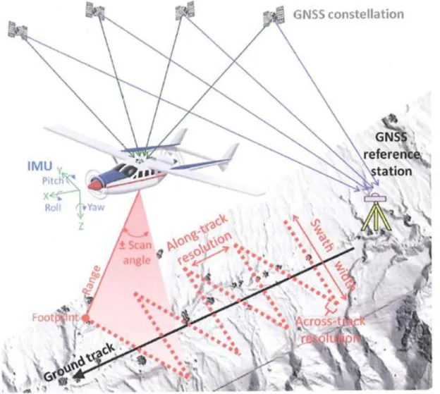
The first uses of airborne mapping LiDAR were as profiling altimeters by the U.S. military in the mid 1960‘s, and included the recording transects of Arctic ice packs and detecting submarines. The first results of topographic mapping with this system were reported in 1984. The basics of airborne mapping LiDAR are illustrated with Figure 5.6. The core of a system is a laser source that emits pulses of laser energy with a typical duration of a few nanoseconds (10-9 s) and that repeats several thousands of times per second (kHz) in what is called pulse repetition frequency (PRF). The laser pulses are distributed in two dimensions over the area of interest. The first dimen¬sion is along the airplane flight direction and is achieved by the forward motion of the aircraft. The second dimension is obtained using a scanning mechanism, which is most often an oscillating mirror that steers the laser beam side-to-side perpendicular to the line of flight. The combination of the aircraft motion and the optical scanning distributes the laser pulses over the ground in a saw tooth pattern. The selected scanning angle and flying height determine the swath width. The scanning frequency, in conjunction with the PRF, determines the across-track spacing of the laser pulses, or the cross-track resolution. The aircraft ground speed and scan frequency determines the down-track resolution. (Fernandez Diaz, J. C., 2011)
Figure 5.7. illustrates that the laser energy spreads in a conical fashion as it propa¬gates through the atmosphere, similar to the pattern of a highly directive spotlight. This spread is determined by the laser beam divergence and, in conjunction with the flying height, defines the size of the beam footprint on the ground. Some airborne systems, such as NASA's Laser Vegetation Imaging Sensor (LVIS), have large footprints of 10-30 m in diameter as they are used to simulate or validate space borne LiDAR sensors. However, most commercial airborne LiDAR units are characterized by beam divergences that produce footprints between 15-90 cm from their typical operational altitudes, and thus are considered "small footprint" systems. Figure 5.7. also illustrates a time-versus-intensity plot, or waveform of a laser pulse propagating in time at the speed of light. When the pulse exits the sensor, it gener¬ally has a nearly Gaussian profile. As the light interacts with the trees or the ground, some of the energy is reflected back towards the sensor, modifying the wave¬form shape according to the geometric properties of the target. The reflected photons are registered by a photo detector, and the signal