Representation transformations of ordered lists ∗
Tibor Ásványi
Eötvös Loránd University, Faculty of Informatics Budapest, Hungary
asvanyi@inf.elte.hu
Submitted September 15, 2014 — Accepted March 5, 2015
Abstract
Search and update operations of dictionaries have been well studied, due to their practical significance. There are many different representations of them, and some applications prefer this, the others that representation. A main point is the size of the dictionary: for a small one a sorted array can be the best representation, while for a bigger one an AVL tree or a red-black tree might be the optimal choice (depending on the necessary operations and their frequencies), and for an extra large one we may prefer a B+-tree, for example.
Consequently it can be desirable to transform such a collection of data from one representation into another, efficiently. There is a common feature of the data structures mentioned: they can be considered strictly ordered lists. Thus in this paper we start a new topic of interest: How to transform a strictly ordered list form one representation into another, efficiently? What about the time and space complexities of such transformations?
Keywords:strictly increasing list, representation-transformation, data struc- ture (DS), linear, array, binary tree (BT), balanced, search tree
MSC:68P05, 68P10, 68P20, 68Q25
1. Introduction
In this paper we consider strictly increasing lists. They can be represented in several different ways. For example, with alinear data structure (LDS)(e.g. array,
∗Supported by Eötvös Loránd University, Faculty of Informatics.
http://ami.ektf.hu
5
linked list, sequential file), with abinary search tree (BST)(e.g. unbalanced BST, AVL tree, red-black tree), with aB-tree,B+-tree, etc. [1, 2, 3].
Their common features are that they can be traversed increasingly in Θ(n) time: the linear traversal of a LDS has linear operational complexity; similarly, the inorder traversal of a tree needsΘ(n)time. And the search-and-update operations can run in O(n)time. [1, 2]
In this paper we use three asymptotic computational complexity measures (each time we consider the worst case by default): O(g(n))(upper bound),Ω(g(n))(lower bound), andΘ(g(n)) =O(g(n))∩Ω(g(n))[2].
Sorted arrayssupport only the search with O(log(n))operational complexity, but for the balanced search tree1 representations each of thesearch, insert, delete operations have this complexity. On linked lists, and sequential files we cannot perform any search-and-update operation inO(log(n))time. Thus we concentrate on the sorted array, and balanced search tree representations of such lists. The search, insert, delete operations have been well studied. Sometimes we have to transform these lists from one representation into another. Consequently we pay attention to these representation-transformations. We ask, how to transform a strictly ordered list Lfrom one representation into another,efficiently?
Undeniably, the operational complexity of such a transformation isΩ(n): each item must be processed. In some cases, it is also O(n): Undoubtedly, a linear representation ofLcan be produced inO(n)time, because the input representation ofLcan be traversed also inO(n)time. Thus, regardless of the input representation of L, a linear representation ofL can be generated withΘ(n)atomic operations.
Besides, a balanced search tree representation ofLcan be generated inO(nlog(n)) time, because a single insert needsO(log(n))atomic operations. Nevertheless this method does not use the information that the input issorted.
Consequently this is our question: Given an input representation ofL, when and how can we produce a balanced search tree representation of it, with an operational complexityΘ(n), or at least better thanΘ(nlog(n))? We give a partial answer to this question. We invent three algorithms. With operational complexityΘ(n), we transform (1) astrictly increasing arrayinto anAVLtree; (2) astrictly increasing array into ared-blacktree; (3) anAVLtree into ared-blacktree.
2. Main results
In order to expound these algorithms (a) we define size-balanced BSTs, and an algorithm transforming astrictly increasing array into such a size-balanced BST;
(b) we prove that a size-balanced BST is almost complete, and so (c) it is anAVL tree; (d) we colour the almost complete BSTs asred-blacktrees; (e) we find a special property ofAVLtrees, and invent an algorithm colouring them as red-blacktrees.
(a-c) are needed for transforming astrictly increasing array into an AVL tree (Section 2.1). (a,b,d) result in the transformation of astrictly increasing arrayinto
1AVL tree, red-black tree, SBB-tree, rank-balanced tree, B-tree, B+-tree, etc.
ared-blacktree (Section 2.2). The theorems and algorithm of (e) in Subsection 2.3 form the high point of this section.
2.1. Strictly increasing array to AVL tree
First we enumerate the necessary notions. By trees we mean rooted ordered trees [2]. Remember thatN IL is the empty tree. The leaves of a nonempty tree have no child. The non-leaves are the internal nodes.
Ift6=N ILis a binary tree (BT),left(t)is its left andright(t)is its right subtree.
If t is a BT, s(t) is its size, i.e. s(t) = 0, if t =N IL; s(t) = 1 +s(left(t)) + s(right(t)), otherwise. h(t) is its height, i.e. h(t) = −1, if t = N IL; h(t) = 1 + max(h(left(t)), h(right(t))), otherwise.
If r is the root node of a BT t 6= N IL, left(r) = left(t), right(r) = right(t), and root(t) =r. Provided thattis a BT,n∈t,ifft6=N IL∧(n= root(t)∨n∈ left(t)∨n∈right(t)).
dt(n)is the depth of nodenin BTt. Ift6=N IL,dt(root(t)) = 0. Ifnis a node of a BT t and left(n) 6= N IL, dt(root(left(n))) = dt(n) + 1. If right(n) 6= N IL, dt(root(right(n))) = dt(n) + 1. Node n is strictly binary (SB(n)), iff left(n) 6= N IL∧right(n)6=N IL.
Clearly, h(t) = max{dt(n) | n ∈ t}, if t 6= N IL. A BT t is complete, iff (∀n∈t)(dt(n)< h(t)→SB(n)).
Notice that for any leafnof a complete BTt,d(n) =h(t); ands(t) = 2h(t)+1−1. A BTtisalmost complete(AC(t)),iff(∀n∈t)(dt(n)< h(t)−1→SB(n)).
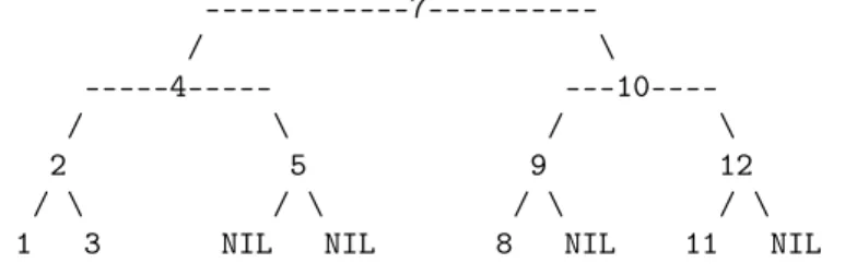
Notice that a BT isAC, iffcompared to the appropriate complete BT, nodes may be missing only from its lowest level: Figure 1 shows such a tree. Clearly, for a leaf nof anAC BTt,dt(n)∈ {h(t), h(t)−1}. The nodes oftat depthh(t)−1 may have one or two children, or may be leaves. s(t)∈[2h(t),2h(t)+1−1].
---7---
/ \
---4--- ---10----
/ \ / \
2 5 9 12
/ \ / \ / \ / \
1 3 NIL NIL 8 NIL 11 NIL
Figure 1: almost complete BST: the places of the missing nodes are shown by NILs
A noden of a BT is height-balanced,iff|h(right(n))−h(left(n))| ≤1. A BT t is height-balanced, iff(∀n ∈t), n is height-balanced. An AVL tree is a height- balanced BST.
A noden of a BT is size-balanced,iff|s(right(n))−s(left(n))| ≤1. A BT t is size-balanced,iff(∀n∈t), nis size-balanced.
We transform a strictly increasing array into an equivalent size-balanced BST in linear time:
We take the middle item of a nonempty array. This will label the root node of the tree. Next we transform the left and right sub-arrays into the appropriate subtrees, recursively. An empty array is transformed into an empty tree.
The resulting size-balanced BST is also an AVL tree, as it follows from the next two theorems.
Theorem 2.1. A size-balanced binary tree is also almost complete (AC).
Proof. We use mathematical induction with respect to the height h(t)of the size- balanced tree t. If h(t) = −1, then t is empty, and AC(t). Let us suppose that we have this property for trees with h(t) ≤ h. Let h(t) = h+ 1. Then t 6= N IL∧h(left(t)) ≤ h∧h(right(t)) ≤ h. It follows by induction that left(t) and right(t)are almost complete. Also|size(left(t))−size(right(t))| ≤1. (Furthermore, remember that a complete binary tree of height hhas the size 2h+1−1, and an almost complete binary tree with size in[2h+1,2h+2−1]has heighth+ 1.) Now we enumerate the possible cases about the subtrees oft, and prove thatAC(t)in each case. If the two (almost complete) subtrees have the same size, their heights are also equal, andAC(t). If the smaller subtree is complete, then the bigger one has an extra leaf at its extra level, and AC(t). If the smaller subtree is not complete, then the bigger one has the same height, andAC(t).
Theorem 2.2. An almost complete binary tree is also height-balanced.
Proof. We can suppose t 6= N IL. First, if AC(t), the leaves of t have depth h(t)or h(t)−1. Thus h(left(t)), h(right(t))∈ {h(t)−1, h(t)−2}. Consequently,
|h(right(t))−h(left(t))| ≤1. As a result,root(t)is balanced. Next, let us suppose thatlr(t)∈ {left(t),right(t)}. Now, ifAC(t), then(∀n∈lr(t))(dt(n)< h(t)−1→ SB(n)). Therefore (∀n ∈ lr(t))(dlr(t)(n) < h(t)−2 → SB(n)). We also have h(lr(t))≤h(t)−1. For these reasons(∀n∈lr(t))(dlr(t)(n)< h(lr(t))−1→SB(n)).
As a result, AC(lr(t)). Thus each (direct or indirect) subtree of t is AC, and if a subtree is nonempty, its root node is balanced. Finally, each node of t is balanced.
Corollary 2.3. A size-balanced BST is also an AVL tree.
Proof. A size-balanced BST is almost complete, thus height-balanced.
Consequently, the algorithm we defined above transforms a strictly increasing array into an equivalent AVL tree. It takes Θ(n)time, because each item of the array is processed once. Besides the Θ(n) size of its output, it needs Θ(log(n)) working memory: this is the height of the recursion. Provided that we need the heights of the nonempty subtrees in their root nodes (as it is usual with AVL trees), we can return the height of a subtree when we return from the appropriate recursive call, and compute the height of a subtree with a given root node from the heights of the two subtrees of that node.
2.2. Strictly increasing array to red-black tree
We have an algorithm transforming a strictly increasing array into an almost com- plete BST. We also have the height of the tree. Here we need an additional flag showing whether the tree is complete or not. Clearly, a nonempty BT is complete, iff its too subtrees are also complete, and their heights are the same. Thus the computation of this flag is also easily merged into the algorithm above.
Next, if we prove that an almost complete BST (with its height and flag) can be coloured in linear time, as a red-black tree, then we have also the algorithm transforming a strictly increasing array into such a tree.
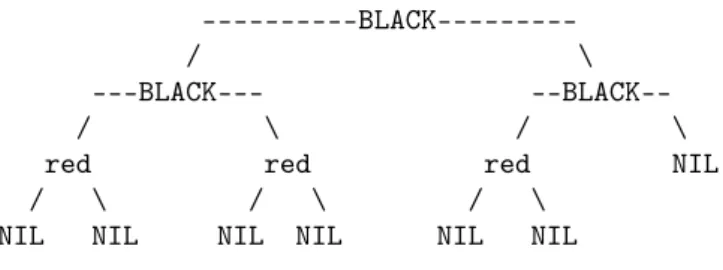
Definition 2.4. A red-black tree is a BST with red and black nodes: The root node is black. We regard NILs as pointers to black, external leaves. For each node, all simple paths from the node to descendant NIL-leaves contain the same number of black nodes. If a node is red, then both its children are black. [2] (See Figure 2.)
---BLACK---
/ \
----red---- --BLACK--
/ \ / \
BLACK BLACK red NIL
/ \ / \ / \
NIL NIL NIL NIL NIL NIL
Figure 2: Red-black tree
Based on this definition, the algorithm of colouring is simple: consider the complete levels of an almost complete BST, and paint the nodes black. If the tree is not complete, the nodes at the lowest, partially filled level remain, and we paint them red. (See Figure 3.) Unquestionably this procedure needs Θ(n) time and Θ(log(n))working memory. The algorithm computing its input (the almost complete tree, its height, and flag) has the same measures. Consequently, the whole transformation has these time and space requirements.
---BLACK---
/ \
---BLACK--- --BLACK--
/ \ / \
red red red NIL
/ \ / \ / \
NIL NIL NIL NIL NIL NIL
Figure 3: Almost complete tree painted as red-black tree
2.3. AVL tree to red-black tree
We colour an AVL tree t as a red-black tree. We use a postorder and a preorder traversal. As a result, our procedure needsΘ(n)time andΘ(log(n))(proportional to the height of t) working memory [1].
Definition 2.5. Minimal height of a binary tree t: m(t) = −1, if t = N IL;
1 + min(m(left(t)), m(right(t))), otherwise.
Theorem 2.6. If t is a height-balanced tree thenm(t)≤h(t)≤2m(t) + 1. Proof. It comes with mathematical induction with respect tom(t). Ifm(t) =−1⇒ t=N IL⇒h(t) =−1⇒m(t)≤h(t)≤2m(t) + 1. Let us suppose that we have this property for trees with m(t) = k. Let m(t) = k+ 1. We can suppose that m(left(t)) =k. By induction: k≤h(left(t))≤2k+1. The treetis height-balanced.
Therefore h(right(t)) ≤ 2k+ 2. Thus k+ 1 ≤ 1 + max(h(left(t)), h(right(t))) = h(t)≤2k+ 3 = 2(k+ 1) + 1. As a result: m(t)≤h(t)≤2m(t) + 1. (Notice that m(t)≤h(t)for any binary tree.)
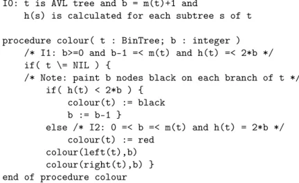
In thecolouringalgorithm, first we calculatem(t). Based on the definition, this can be done with a postorder traversal oft. In a typical AVL tree, for each non-NIL subtree soft, theh(s)attributes are already present. (If not, the computation of theh(s)values can be easily merged into the postorder traversal.)
Next, with a preorder traversal of t, we colour t. (See Figure 4). We paint m(t) + 1nodes black on each simple path from the root to a NIL-leaf. (The NIL- leaves are also considered black, but we do not paint them.)
PreCondition of the first call:
I0: t is AVL tree and b = m(t)+1 and
h(s) is calculated for each subtree s of t procedure colour( t : BinTree; b : integer )
/* I1: b>=0 and b-1 =< m(t) and h(t) =< 2*b */
if( t \= NIL ) {
/* Note: paint b nodes black on each branch of t */
if( h(t) < 2*b ) { colour(t) := black b := b-1 }
else /* I2: 0 =< b =< m(t) and h(t) = 2*b */
colour(t) := red colour(left(t),b) colour(right(t),b) } end of procedure colour
Figure 4: Colouring an AVL treetas a red-black tree
Now we are going to prove the correctness of thecolouringalgorithm in Figure 4.
Terminology: In the rest of this section we useI0(i.e. the PreCondition), invari- antsI1,I2, and other logical statements. Let us suppose thatIj, Ik∈ {I0, I1, I2}; P,Qare arbitrary statements. When we say thatIj withP inducesIkwithQ, we mean: IfIj andP are true when the program is at the place ofIj, thenIkandQ will hold when the run of the program next time arrives at the place ofIk.
Lemma 2.7. I0 inducesI1 withh(t)<2b.
Proof. Based on the definition of m(t), m(t) ≥ −1. Consequently b = m(t) + 1 impliesb≥0∧b−1≤m(t). Theorem 2.6 impliesh(t)≤2m(t) + 1. Considering b=m(t)+1we receiveh(t)≤2m(t)+1 = 2(b−1)+1 = 2b−1. Thush(t)<2b. Lemma 2.8. I1 with t6=N IL∧h(t)<2b inducesI1 in both recursive calls.
Proof. Lets(t)be the left or right subtree parameterizing the appropriate recursive call. Thus we need to prove I1b←b−1,t←s(t) i.e. that the following three conditions hold:
(1) b−1 ≥0: We know thath(t)≥0 (since t 6=N IL) and h(t) <2b. Conse- quently,b >0, and thereforeb−1≥0.
(2) b−2 ≤ m(s(t)): From I1, b−1 ≤ m(t). From the definition of m(t), m(t)≤1 +m(s(t)). As a result, b−1≤1 +m(s(t)), i.e. b−2≤m(s(t)). (3) h(s(t)) ≤ 2(b−1): h(t) < 2b, i.e. h(t) ≤ 2b−1; h(s(t)) ≤ h(t)−1; thus
h(s(t))≤2b−2.
Lemma 2.9. I1 with t6=N IL∧h(t)≥2b inducesI2.
Proof. h(t)≤2b andh(t)≥2bimpliesh(t) = 2b. 0≤b remains true. Considering Theorem 2.6 we have2b≤2m(t) + 1; thusb≤m(t) + 1/2 i.e.b≤m(t).
Lemma 2.10. I2 inducesI1with h(t)<2b in both recursive calls.
Proof. Lets(t)be the left or right subtree parameterizing the appropriate recursive call. Thus we have to prove (I1∧h(t)<2b)t←s(t) i.e. b ≥0∧b−1 ≤m(s(t))∧ h(s(t))<2b. b≥0 remains true. Fromb≤m(t)andm(t)≤1 +m(s(t))we have b−1≤m(s(t)). h(t) = 2bimpliesh(s(t))<2b.
Theorem 2.11. Provided that the precondition I0 holds, procedure colour paints the nodes of tree t so thatt becomes a red-black tree.
Proof. Lemmas 2.7, 2.8, 2.9, and 2.10 imply that I1 andI2 are invariants of the program. I1means that when we arrive at an external leaf, i.e.t=N IL,0≤b≤ m(t) + 1 =−1 + 1, as a resultb= 0. In the programbis decreased (by 1), exactly when a node is painted black. Because b is decreased to zero on each branch of any subtree while we go to a NIL-leaf, we have the same number of black nodes on these paths. Lemma 2.7 implies that the root node of the tree is painted black.
Lemma 2.10 makes sure that both children of a red node will also be black. These have the effect of receiving a red-black tree.
Let acrb-tree be a BST which can be coloured as a red-black tree. Then an AVL tree is also a crb-tree. This also follows from both of the following results.
(1) Bayer proved that the class ofSBB-treesproperly contains the AVL trees [4], and we know from 4.7.2 in [3] that the SBB-trees and the red-black trees are structurally equivalent.
(2) Rank-balanced trees are a relaxation of AVL trees, and form a proper subclass of crb-trees [5].
Our achievements and these results are unrelated. In this subsection our contribu- tions are the notion of the minimal height of an AVL tree, theorems 2.6 and 2.11, and ourefficient colouring algorithmproved.
3. Conclusions
This was our question: How to transform a strictly increasing list L from one representation into another,efficiently?
Summarizing this paper, we already know that given an input representation of L, we can produce another representation of it in Θ(n)time, if this other rep- resentation is a linear data structure, an AVLor red-blacktree. In some cases we have direct transformations, in other cases we need a temporary array.
In three cases we invented the necessary algorithms, theorems, lemmas, and proofs. The first two, (sorted array →balanced BST) programs create new trees;
but the second half of the second algorithm, and the third (AVL tree→red-black tree) procedure do not make structural changes on the actual tree, just paint its nodesblack, andred. Each of the three programs needsΘ(log(n))working memory.
Our algorithms and theorems imply three relations among four classes of BSTs:
size-balanced BSTs ⊂ almost complete BSTs ⊂ AVL trees ⊂ crb-trees. Actually, each of the first three classes is a proper subclass of the next one. For exam- ple2 BST (((1)2(3))4(5)) is almost complete, but not size-balanced; AVL tree ((((1)2)3(4))5(6(7)))is not almost complete; red-black tree((1b)2b((3b)4r(5b(6r)))) is not height-balanced.
Open questions: IfLis transformed into another type of balanced search trees (notinto an AVL orred-black tree); for example, into a B-tree, we know that the operational complexity of the transformation is Ω(n), and O(nlog(n)). Here we still need more sharp results. Maybe, from a strictly increasing list, each kind of balanced search trees can be generated inΘ(n)time? Are there some cases, when the time complexity is more thanΘ(n), but less thanΘ(nlog(n))?
If the input representation ofLis a search tree (or a linked list or a sequential file), and the output is anAVLor red-blacktree, we can make the transformation in Θ(n) time, but – with the exception of theAVL tree→red-black tree program
2Using the notation(left-subtree root right-subtree)where the empty subtrees are omitted.
– we actually need a temporary array, thusΘ(n)working space. We ask: In which cases can we reduce the memory needed?
References
[1] Weiss, Mark Allen, Data Structures and Algorithm Analysis, Addison-Wesley, 1995, 1997, 2007, 2012, 2013.
[2] Cormen, T.H., Leiserson, C.E., Rivest, R.L., Stein, C.,Introduction to Algo- rithms,The MIT Press, 2009. (Ebook: http://bit.ly/IntToAlgPDFFree)
[3] Wirth, N., Algorithms and Data Structures,Prentice-Hall Inc., 1976, 1985, 2004.
(Ebook: http://www.ethoberon.ethz.ch/WirthPubl/AD.pdf)
[4] Bayer R.,Symmetric Binary B-Trees: Data Structure and Maintenance Algorithms, Acta Informatica 1, 290–306 (1972),Springer-Verlag, 1972.
[5] Haeupler B., Sen S., Tarjan R.E., Rank-Balanced Trees, Algorithms and Data Structures: 11th International Symposium, WADS 2009, Banff, Canada, August 2009, pp 351–362,Springer-Verlag, LNCS 5664, 2009.