CHAPTER ELEVEN HETEROGENEOUS EQUILIBRIUM

CHAPTER ELEVEN

HETEROGENEOUS EQUILIBRIUM

Equilibria involving two or more phases—heterogeneous equilibria—have been discussed at various points in preceding chapters. The function of the present chapter is to organize examples of such systems according to a more formal frame­

work and to extend the complexity and variety of systems considered. The thermo­

dynamic criterion for equilibrium finds a more general form known as the Gibbs phase rule. There will be considerable emphasis on graphical methods for representing phase equilibria. Graphs showing pressure-temperature-composition domains for phases were called phase maps in preceding chapters; the more common term of phase diagram will now be used.

11-1 The Gibbs Phase Rule

The criterion for phase equilibrium was developed in Section 9-3C, where it was concluded that the chemical potential of each component must be the same in all phases. Thus for two phases in equilibrium the condition for the ith component is

μ*^α = = - [Eq. (9-44)],

where α, β, and so on denote the various phases in equilibrium. The effect of this condition is to reduce the number of independent variables that are needed to specify the state of the system.

Consider first the case of a pure substance. If it is present as a single phase a, then we must specify pressure and temperature to fix the state of the substance.

That is, we write

μ*=ηΡ,Τ) (11-1) and phase α will have a region of existence over some range of Ρ and Γ, as is

illustrated in Fig. 8-12. The same is true for some second phase β:

μ'=/*(Ρ⁹ T). (11-2)

391

(It would be perfectly acceptable to use G* and G⁰ instead of μ* and μ^β, since composition is not a variable, but it seems better to keep a uniform nomenclature.)

Equilibrium between the two phases corresponds to a line of crossing of the surfaces generated by /^a and f^e in the three-dimensional plots of μ versus Ρ and T.

In effect we solve Eqs. (11-1) and (11-2) simultaneously to obtain as the condition of phase equilibrium

f^a(P, T) = f*(P, T) or Ρ = φ«\Τ). (11-3)

There is now only one degree of freedom; that is, one independently variable intensive quantity determines the state of the system having two phases present.

If a third phase γ is possible, then for α-y equilibrium we have

MP, T) = f*(P, T) or Ρ = φ«ν(Τ). (11-4) We now ask that all three phases be in equilibrium, that is, coexist at the same

Ρ and T. We obtain the condition by solving Eqs. (11-3) and (11-4) simultaneously.

With two unknowns (P and T) and two equations, the solution gives unique values for pressure and temperature. The number of degrees of freedom is now zero.

A system consisting of a single substance is called a one-component system, meaning that its composition is fixed. A system in which the amounts of two substances must be specified for composition to be fixed is called a two-component system. The statements of chemical potential for phase α are now

μι^α = fi*(P, T, ^Xl«) and 첫 = /²«(P, Γ, xf), (11-5) where the subscripts identify the components and χ is mole fraction. Since Xi + x² = 1, it is simpler to eliminate x² immediately in writing the second of Eqs. (11-5). There are three degrees of freedom in this case; we must specify Ρ, Γ, and x^x in order to define the state of the system.

If two phases α and β are in equilibrium, then

/ V = μι and 첫 = μ^2β, (11-6)

or

Τ, ^Xl*) = / / ( Ρ , Τ, xf) and /²° ( P , Γ, xf) = f²%P, Γ, xf). (11-7) There are now four variables, Ρ, T, xf, and xf, and two equations, so that two of the variables are no longer independent; there are two degrees of freedom. In the case of an equilibrium between a solution and its vapor, we customarily choose Τ and x^l) as the independent variables. If these are specified, then both the total vapor pressure and the vapor composition are determined.

The general case is developed as follows. If a system has C components, then the number of variables required to define its state will be two (P and Γ), plus (C — 1). That is, C mole fractions are involved, one of which is immediately eliminated by the condition that their sum must be unity. The total number of variables is

number of variables = ^ ( C - 1) + 2, (11-8) where 9 denotes the number of phases in equilibrium (see Section 11-CN-l).

11-2 ONE-COMPONENT SYSTEMS 393

The condition for equilibrium generates the equations μ* = = = = ...,

μ

= μ£ = μ<? = μ

= - , C

"

)

or — 1 equations for each component. The total number of equations is

number of equations = C{& — 1). (11-10) The number of degrees of freedom is the difference between Eqs. (11-8) and (11-10),

F = 0>(C - i ) + 2-C(0>- 1), or

F + & = C + 2. (11-11) Equation (11-11) is known as the Gibbs phase rule.

The phase rule is useful in several ways. It tells us the maximum possible number of equilibrium phases that can coexist. In the more complex systems it helps to determine the number of components present and whether the phases present are well behaved. This aspect is discussed further in the Commentary and Notes section; for the present it is sufficient to make the following definitions:

Number of components: the minimum of compositions needed, along with pressure and temperature, to define the state of the system;

Number of phases: the number of different kinds of states of matter present.

Number of degrees of freedom: number of independently variable intensive quantities whose values must be fixed to determine the state of the system.

11-2 One-Component Systems

One-component systems were summarized in Chapter 8. The phase rule reduces to F+ & = 3. We may have single phases existing over a region of Ρ and Γ, two-phase equilibria governed by the Clapeyron (or Clausius-Clapeyron) equation and thus defined by a Ρ - Γ line, and three-phase equilibria characterized by a triple point, or unique values of Ρ and T. If η phases are known, there will be n(n — l)/2 lines of two-phase equilibria; this is the number of distinguishable ways of picking two out of η objects. Also, there will be n(n — l)(n — 2)/3!

possible triple points.

From the graphical point of view, a three-dimensional model is needed; one must show μ = / ( Ρ , Τ), as in Fig. 8-12, or the equation of state of each phase V = g(P⁹ Γ), as illustrated in Fig. 1-9. One may take various cross sections of the three- dimensional plot, usually either isothermal or isobaric ones. The surfaces of state for gaseous, liquid, and solid water intersect to give gas-liquid, gas-solid, and liquid-solid lines, which in turn intersect at the triple point.

Two-phase equilibria can, of course, be shown as Ρ versus Γ plots, as in Fig. 8-3 for vapor pressures. A set of two-phase equilibrium lines constitutes a phase

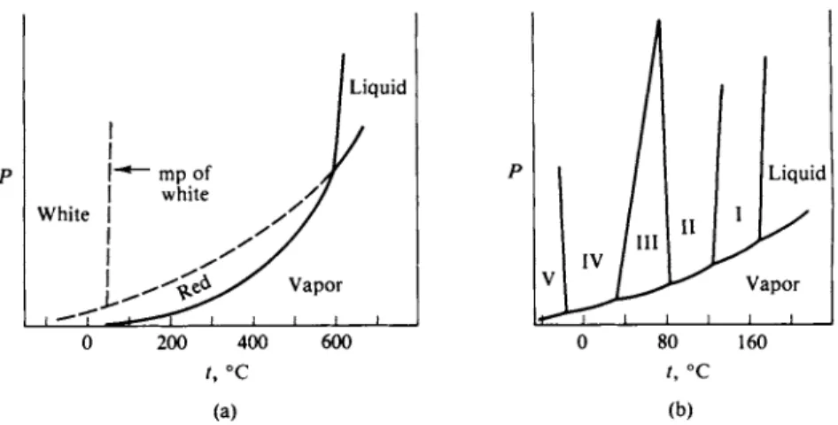
F I G . 1 1 - 1 . (a) Phase diagram for phosphorus, (b) Phase diagram for N H⁴N O^s [see R. G. Early and Τ. M. Lowry, J. Chem. Soc. 1387 (1919)].

diagram, as in Figs. 8-8b and 8-11. Two additional systems are shown in Fig. 11-1.

That for phosphorus (a) illustrates a case where, although two solid forms are known, only one is ever stable. White phosphorus may be prepared chemically but is always unstable with respect to red phosphorus. The ammonium nitrate system (b) is one in which a rather long succession of crystal modifications occur, each with a region of stability.

11-3 Two-Component Systems

The phase rule for a two-component system is given by F + & = 4. A four-dimen­

sional plot would be needed to show the state of a two-component system, that is, to plot Eqs. (11-5) or to show V = g(P, T, xj. One must therefore proceed immediately to one or another cross section, or use tabulations. Our interest, however, is in phase equilibria. The equilibrium between two phases can be shown as a Ρ-Γ-composition plot or three-dimensional model, as in Fig. 9-14. These are awkward to use, so in actual practice one customarily takes either isothermal or isobaric cross sections. The vapor pressure-composition diagrams of Chapter 9 are examples of the former, and the boiling point diagrams are examples of the latter.

Figure 7-2 similarly shows isothermal and isobaric cross sections for the C a O - C 0² system and Fig. 9-20 shows an isobaric cross section depicting the equilibrium between two partially miscible liquids. The freezing point depression equation (10-15) gives the line of equilibrium between a solution and a pure solid for a constant pressure of 1 atm.

These examples represent isolated portions of various phase diagrams, and the material that follows will assemble these various portions into a more complete picture. Boiling point diagrams were covered in Section 9-6 and the emphasis here will be on freezing point and solubility diagrams. Solid phases will be taken to be immiscible; some cases of partial miscibility are considered in Section 11-ST-l.

11-3 TWO-COMPONENT SYSTEMS 395 A. Freezing (or Melting) Point Diagrams

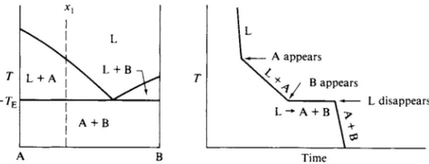
We consider the simplest case first, namely, that in which the miscibility gap essentially coincides with the A and Β sides of the diagram, that is, the case of complete immiscibility. If the liquid solution is ideal, then the solution-solid equi­

librium line is given by the freezing point depression equation (10-15). This equation is plotted in Fig. 11-2, assuming first that pure solid A separates out; line ab results.

A system of this type is symmetric, and the freezing point of liquid Β will similarly be lowered by the presence of dissolved A. This second freezing point depression curve is shown by line cd in the figure. At the point of crossing of these two lines solution of composition x^E is simultaneously in equilibrium with pure solid A and pure solid B. On attempted cooling, the system can pursue neither the dashed extension of ab nor that of cd without departing from equilibrium with respect to either solid Β or solid A. The consequence is that the temperature must remain invariant at T^E so long as the three phases are present. This invariance is demanded by the phase rule—the one degree of freedomhaving been used in setting the pressure at 1 atm.

The completed phase diagram is shown in Fig. 11-3; it is called a eutectic diagram. The temperature T^E is the eutectic temperature and x^E the eutectic com­

position. The phase map aspect may be developed as follows. A solution (or melt, if the system is a high-temperature one) of composition x¹ will begin to freeze at T^x. With further cooling, solid A appears, and at some temperature T² the system consists of solid A and liquid of composition x². The proportions are given by the lever principle (Section 9-2C). The lengths l^x and l² of the two sections of the tie-line at T² are in the same proportion as are the amounts of solution and of solid:

klk ⁼ (amount of solution)/(amount of solid).

If composition is plotted as mole fraction, the ratio will be of the number of moles of solution to the number of moles of solid; and if composition is in weight fraction or percent, the ratio will be that of weight of solution to weight of solid.

At T^E the solution has reached composition x^E , and further withdrawal of heat leads to the simultaneous freezing out of solid A and solid B. Since the solution

A * B Β F I G . 11-2. Freezing point diagram for an ideal solution.

Ά

τ

A J CB Β F I G . 1 1 - 3 . Application of the lever principle.

cannot change composition, the proportion of A and Β in the mixed solids must be given by J C^e . The eutectic solid is thus one of definite composition, and perhaps for this reason it has sometimes been misnamed a eutectic compound. It is not a compound; its composition varies with pressure, for example. In the case of metal systems especially the superficial appearance of the eutectic mixture may be that of a single phase, but microscopic examination shows a mechanical mixture of small crystals of the two pure phases.

Eventually the liquid phase disappears and the system consists of solid A and solid Β in overall proportion corresponding to x¹.

Cooling of a liquid of composition x^x' gives the same general sequence of changes.

The first phase to separate out is now pure solid B, however. At T^E both A and Β freeze out together, and when the liquid phase has disappeared one has the mixed solid phases of overall composition

B. Cooling Curves for a Simple Eutectic System

The preceding system is called a simple eutectic one, for reasons that are made especially apparent in the Special Topics section; freezing point diagrams can take on a rather complicated appearance. Simple eutectic, as well as the more complex systems, may be studied by what is known as the method of thermal analysis. The experiment consists in placing the liquid solution or melt in a container from which heat is withdrawn at a steady rate. That is, dq/dt is kept approximately constant.

The liquid has a certain heat capacity C^P(l) and the rate of change of its temperature with time is

dT _ 1 dq

dt C^P(l) dt (11-12)

(dq⁹ and hence dT/dt⁹ is negative since the system is losing heat). If we suppose the solution to be of composition x^x in Fig. 11-3, then at T^x solid A begins to freeze out. This means that its latent heat of freezing AHf^tA is liberated. The shape of the line ab [Fig. 11-2] determines dnJdT, that is, the number of moles of A appearing

11-3 TWO-COMPONENT SYSTEMS 397

per unit temperature drop. Due to this effect, heat is supplied to the system at the rate

%=-*K^.

The consequence is that the heat capacity of the system is increased by an amount C^Pti, and the net heat capacity becomes

C^P(net) = C^P( / ) «^L + AHU ^ + C^P(A)n^A , (11-14) where n^L and n^A are the number of moles of liquid and of solid A present respec­

tively. The rate of cooling is therefore reduced.

A schematic cooling curve for composition x^x is shown in Fig. 11-4. The slope of the first section is given by Eq. (11-12). At T^x (see Fig. 11-3) the slope changes to one determined by C^P(net); the cooling line is actually curved since C^F(net) changes with the relative amounts of liquid and solid phase. At T^E the temperature remains constant; the removal of heat now goes to freezing out A and Β together.

At the end of the halt, liquid phase has disappeared, and cooling resumes, with dT/dt given by Eq. (11-12) but with a heat capacity corresponding to that of the mixture of solids:

C^P( A + B ) = n[^XlC^B + (1 - ^{X l}) C^A] , (11-15) where η denotes the total number of moles of the system. Experimental cooling

curves may show small temperature minima at breaks and halts, due to supercooling.

It helps to define exactly what is happening along each section of a cooling curve if the phase or phases present are indicated as is done in Fig. 11-4. A halt corresponds to a so-called phase reaction, that is, to the physical process of inter- conversion of phases. In the present example, the phase reaction is L —• A + B.

One should also show at each break what phase or phases are appearing or disap­

pearing.

Figure 11-5 shows a series of cooling curves for various initial compositions of the system of Fig. 11-3. Notice that the locus of the temperatures of the first break defines the freezing point lines [ab and cd in Fig. 11-2]. The unique halt temperature identifies the system as one having a single eutectic, and the cooling curve of composition labeled JC³ identifies the eutectic composition since preliminary separation of neither A nor Β alone occurs.

A ^X\ x² *³ x^A Β

A Β Time F I G . 11-5. Set of cooling curves.

The relative lengths of the various sections of the cooling curves should also be consistent with the phase diagram. Suppose, for simplicity, that there is always one mole total of system. The length of the halt for the cooling of pure liquid A is then AH^f°^Al(dqldt) and that for the cooling of pure liquid Β is AH^f°^Bl(dqldt). For inter­

mediate compositions the length of the eutectic halt is proportional to n^E, the amount of eutectic solution that must freeze out. Returning to Fig. 11-3, we see that n^E = /³/ ( /³ + /⁴) . Clearly, the closer the initial composition is to x^E , the greater will be this proportion, and the longer will be the halt in the cooling curve. An alternative way for one to locate the eutectic composition is then to plot the length of halt against initial composition and extrapolate both sections to find the maxi­

mum. One thus avoids having to hit the composition J C^e exactly in a series of ther­

mal analysis experiments.

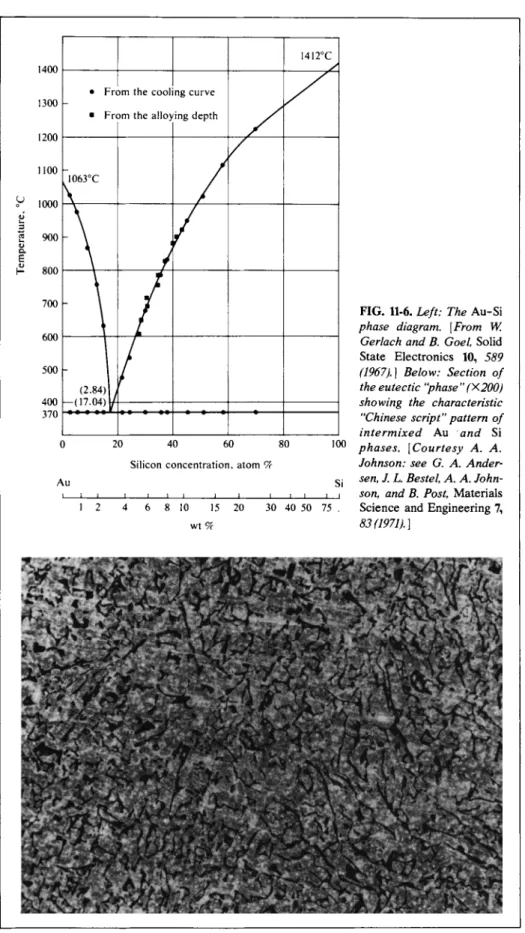
Simple eutectic behavior is illustrated by the Au-Si system, shown in Fig. 11-6.

The gold-silicon junction is an important one in the semiconductor industry and the composition and morphology of the eutectic " p h a s e " have been much studied.

C. Compound Formation

It happens quite often that the two components form one or more solid com­

pounds—AB, A²B , A B², and so on. If these are stable, they show a normal melting point, or are said to melt congruently. The effect is simply to divide the phase diagram into as many separate sections. This is illustrated in Fig. 11-7 for the case of a compound A B². The two eutectics have no necessary connection with each other, nor, in fact, do any aspects of the two portions of the diagram. Each may be treated separately.

What sometimes happens, however, is that a compound decomposes to give liquid and one of the other solid phases. Figure 11-7 would now take on the appearance of Fig. 11-8, where compound A B² decomposes at T^d to give liquid of composi­

tion x^a and solid B. Such a decomposition is called an incongruent melting, meaning that the liquid is not of the same composition as the solid and avoiding the impli­

cation of irreversibility suggested by the term decomposition. It is helpful at this point to label the various phase regions. This not only clarifies the geography of the phase map but is of direct use in the construction or interpretation of cooling curves. The general rule is that a break occurs when, on cooling, the system com­

position line passes from one type of phase region to another, such as on cooling

11-3 TWO-COMPONENT SYSTEMS 399

ε

1400

1300

1200

1100

1000

900

800

700

600

500

400 370

1412°C

• F n

• Fr<

)m the cool 3m the alloy

ng curve ing depth

1063°C

A /

(2.84)

—(17.04) ^(2.84)

1 /

—(17.04)

f

20 40 60 80 Silicon concentration, atom %

100

Au

1 2 10 15

wt %

20 30 40 50 75

FIG. 11-6. Left: The Au-Si phase diagram. [From W.

Gerlach and B. Goel, Solid State Electronics 10, 589 (1967).] Below: Section of the eutectic "phase" (X200) showing the characteristic

"Chinese script" pattern of intermixed Au and Si phases. [Courtesy A. A.

Johnson: see G. A. Ander­

sen, J. L. Bestel, A. A. John­

son, and B. Post, Materials Science and Engineering 7, 83(1971).]

along the x¹ line shown in Fig. 11-8. A halt must occur when a line of three- phase equilibrium is reached, and cooling must resume when a two-phase or a one-phase region is entered.

Systems of composition x^x and x² show normal eutectic cooling curves, but the behavior of the curve for x³ is more complex. Solid Β begins to separate out at 7\

and at Τ^ά the solution has reached composition x^d and is now in equilibrium with both solid Β and compound C ( = AB²). There must therefore be a halt in the cooling curve until at least one of the three phases disappears.

The phase reaction that occurs at Τ^ά may be determined as follows. Just above T^d the phases present are L and B ; just below T^d they are L and C. Evidently Β disappears and C appears. However, Β cannot by itself produce C, and the phase reaction is evidently L + Β —• C. We may confirm this by noting that for com-

F I G . 11-7. The case of compound formation.

F I G . 11-8. (a) Unstable compound formation, (b) Cooling curves.

11-3 TWO-COMPONENT SYSTEMS 401 position x^z, use of the lever principle shows that the proportion of L present decreases when the three-phase line is traversed.

After the halt at T&, the system x^z consists of L + C, and further cooling freezes out more C until T^E is reached. At this point the liquid is at x^E and the rest of the cooling curve is the same as for the simple eutectic case.

Finally, a system of composition *⁴ traverses the T& line on cooling but then enters the C + Β phase region. The phase reaction is always the same anywhere along a three-phase line, but what now happens is that as the process L + Β -> C occurs it is the liquid phase which is used up first.

D . Rules of Construction

Although not important for the relatively simple diagrams considered here, there are some rules that assist in the construction and labeling of more complicated diagrams. A two-component phase diagram consists of one-phase and two-phase regions and lines of three-phase equilibria. The latter always connect the three compositions of the three phases that are in equilibrium and must, of course, be mathematically horizontal lines. There will always be two end phases and one of intermediate composition, and a first rule is that the end phases are always present both above and below the temperature of the three-phase line. The phase of inter­

mediate composition may exist only above the line, as in eutectic diagrams, or only below the line, as with C in Fig. 11-8. In this case the line is called a peritectic line.

Alternatively, a line of three-phase equilibrium is a boundary for three two-phase regions. There are two such regions above a eutectic line and one below it; con­

versely, there is one such region above a peritectic line and two regions below it.

A second rule is that a horizontal traverse must encounter alternate one-phase and two-phase regions. In applying the rule to a diagram such as that of Fig. 11-8, we regard pure A, pure C, and pure Β as very narrow one-phase regions. The reader is encouraged to test the various two-component diagrams of this chapter against these rules.

11-4 Sodium Sulfate-Water and Other Systems

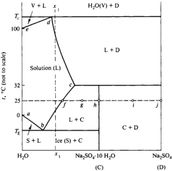
A specific system that both illustrates and extends a number of the points discussed in the preceding section is that for sodium sulfate and water. The usual phase diagram is shown in Fig. 11-9 and displays the following features. The lower left curve ab is the ordinary freezing point depression curve for aqueous sodium sulfate solutions. Curve be is the solubility curve for N a²S O⁴1 0 H²O , showing a normal increasing solubility with increasing temperature. (The curve can be viewed alternatively as the freezing point depression curve of N a²S O⁴1 0 H²O , as discussed in Section 10-CN-2.) This region of the diagram then shows a simple eutectic behavior, Γ^Ε being at — 1.3°C, and the eutectic solution being 0.33 m in sodium sulfate. As an item of incidental information, a eutectic involving ice as one of the solid phases is often called a cryohydric point.

The decahydrate decomposes at 32.4°C to give the anhydrous salt whose solu­

bility curve is given by cd. The situation is that of unstable compound formation

and the three-phase line at 32.4°C is therefore of the peritectic type. The diagram is schematic in that both the temperature and the composition scales have been somewhat distorted so as to display the various phase regions more clearly. These are labeled, however, and a cooling curve, such as for the system of composition x¹, leads to the sequence of phase changes determined by the regions traversed; it will show the usual eutectic halt at T^E .

In a system of this type one of the components is relatively volatile, and one may consider an evaporation sequence. For example, if a dilute sodium sulfate solution is evaporated at 25°C the system will traverse the horizontal line shown in Fig. 11-9.

τ

'c 100

υ

V + L χ H20 ( V ) + D

< V

S o l u t i o n (L) \

L + D

\ / I L + C

Χ*/ ι

i j

C + D

/ j

S + L Ice (S) + C 32

25

H²0 x\ N a2S O⁴1 0 H²O

(C)

FIG. 11-9. The H²0 - N a²S 0⁴ system for 1 atm pressure.

N a²S 0⁴ ( D )

Saturation with respect to N a²S O⁴1 0 H²O occurs at system composition / , and continued evaporation deposits solid N a²S O⁴1 0 H²O in increasing amounts. When the overall composition has reached point g, solution / and solid decahydrate are present in amounts given by the lever principle. At system composition h, solution has disappeared and only N a²S O⁴1 0 H²O is present. Further evaporation—or removal of water—begins to transform the solid into anhydrous salt; at system composition i there would be about equal parts of N a²S O⁴1 0 H²O and N a²S 0⁴ . At point7, of course, only the anhydrous salt is present.

We now turn to the higher-temperature region of the diagram. Pure water is in equilibrium with vapor at 100°C, this being the diagram for 1 atm pressure, and there is a boiling point elevation with increasing salt concentration, given by line de. At the intersection of lines de and cd, solution, vapor, and N a²S 0⁴ are in equilibrium, and above T^c the solution has evaporated to give water vapor and solid N a²S 0⁴.

11-4 SODIUM SULFATE-WATER AND OTHER SYSTEMS 403

V + D V + L

1

C + D

^ T ^ /

C + D S + L S + C

C + D

(a)

V + D

(b)

F I G . 11-10. Effect of reduction of pressure on the phase diagram for the H²0 - N a²S 0⁴ system.

T h e boiling point and therefore also T0 decrease with decreasing pressure. A t a sufficiently l o w pressure, the phase diagram takes o n the appearance s h o w n in Figure 11-10(a). T h e deca- hydrate n o w d e c o m p o s e s at Γ⁰' t o give water vapor a n d the anhydrous salt. A t o n e particular pressure T⁰ = 7 V , a n d at this temperature four phases, K, L , C , a n d D , can b e in equilibrium, as s h o w n in Fig. l l - 1 0 ( b ) . This is the quadruple point for the system.

There is a large variety of phase diagrams of the salt hydrate type. Another common one is for the H²0 - F e C l³ system, shown in Fig. 11-11. A succession of hydrates exists, each melting congruently. An interesting exercise is to trace out the series of changes occurring on evaporation of a FeCl³ solution at a temperature just below the melting point of the heptahydrate (see Problem 11-19). An example of 1:1 compound formation involving organic compounds is provided by the p- equally interesting is the H²0 - H²S 0⁴ phase diagram. A very simple example of 1:1 compound formation involving organic compounds is provided by the /?- toluidine-phenol system shown in Fig. 11-12; the C a F²- C a C l² system shown in Fig. 11-13 illustrates unstable compound formation.

F I G . 1 1 - 1 1 . The H²0 - F e C l⁸ system.

F I G . 1 1 - 1 2 . The p-toluidine-phenol system.

F I G . 1 1 - 1 3 . The C a F²- C a C l² system, showing unstable C a F²- C a C l²

compound formation.

11-5 THREE-COMPONENT SYSTEMS 405

11-5 Three-Component Systems

A. Graphical Methods

Some formidable problems of representation develop with three-component systems. Graphing of the equation of state V = g(P⁹ Γ, x^x, x²) now requires five-dimensional space! The requirement is reduced to a four-dimensional one if two-phase equilibria are to be shown over a region of existence. Fortunately, or perhaps because of this difficulty, most studies of three-component systems have been carried out with only condensed phases present so that pressure is not an important variable, and isobaric diagrams supply the important information. These are three-dimensional, and their use is awkward but feasible. The chemical engineer who deals with the distillation of multicomponent systems has a problem that we will not consider here.

In an isobaric phase diagram two coordinates are used to fix composition and a third is used to fix the temperature. There are various ways in which the com­

position of a ternary or three-component system may be plotted, the choice being made in terms of the type of system. A very convenient one makes use of the properties of an equilateral triangle. As illustrated in Fig. 11-14, one of these properties is that the sum of the perpendicular distances to an interior point, ad + bd + cd, is always equal to the altitude of the triangle h. Triangular graph paper is therefore ruled with three sets of lines, each set parallel to one of the bases. A point such as d may then be read as having the coordinates 50 % h^A , 20 % h^B , and 30 % h^c . The coordinate system is then used to express composition.

For example, point d would be the pivot or balance point for the triangle if weights in the proportion 50:20:30 were hung from the A, B, and C corners, respectively.

Point d thus corresponds to a system of composition 50 % A, 20 % B, and 30 % C.

A valuable feature of the triangular graph is that addition of one of the com­

ponents will cause the system composition to move along the line drawn between it and that corner. Thus addition of C to a mixture of composition d will produce the

c

h

A Β

F I G . 1 1 - 1 4 . Triangular coordinate paper.

F I G . 11-15. A simple ternary eutectic system.

succession of new compositions along the line dC. The lever principle applies. Thus at point e the ratio of the amount of added C to the amount of original mixture is If C is removed from mixture d (by evaporation or freezing), the composition of the remaining mixture will move t o w a r d / , still on the dC line. It is not necessary that the added or removed material be pure component. The line connecting any two compositions is the locus of all mixtures of such compositions. For example, point e happens to be on the line connecting points a and b. Addition of mixture a to mixture e would move the system composition along the aeb line, toward a.

Alternatively, mixture e could be made up by the combination of a and b in the proportions given by the lever principle.

B . The Simple Ternary Eutectic Diagram

Isobaric diagrams may be constructed with a coordinate system based on the equilateral triangular prism, with temperature measured along the prism axis. Each face of the prism constitutes a two-component system; the three faces thus show the A - B , B-C, and A - C phase diagrams. This is illustrated in Fig. 11-15 for a simple eutectic system, that is, one in which A, B, and C are fully miscible in the liquid phase but are essentially immiscible in the solid state.

11-5 THREE-COMPONENT SYSTEMS 407 Examination of the figure shows, for example, that the freezing point T^AC of the binary eutectic solution ac is further lowered on addition of Β to the system. The composition of the series of freezing A - C eutectic solutions moves along the line ac-abc. There is a corresponding depression of the be eutectic by the addition of A and of the ab eutectic by the addition of C. The three freezing point depression curves for the three binary eutectic solutions meet at point abc at T^ABC . This is the quadruple point of the diagram; at T^ABC solids A, B, and C are in equilibrium with solution of composition abc.

The sequence of events on cooling of a solution of composition (1) is also shown.

At temperature 7\ , or point e on the diagram, C begins t o freeze out, and the solution composition moves along the dashed line ef. When it reaches the ac-abc line and temperature Γ³, solid Abegins to freeze out as well,andwith further cooling A and C freeze out together while the solution composition moves toward abc.

At T^ABC the solution is of composition abc and is now also saturated with respect to B. The system is invariant at this point and the temperature remains constant while A, B, a n d C freeze out together. Cooling resumes when the solution has disappeared.

It is necessary to work with isothermal sections of the diagram if the analysis is to be more accurate. A succession of these is shown in Fig. 11-16; the temper­

atures correspond to those marked in Fig. 11-15. The section at T^x, Fig. 11-16(a), cuts the three "cloverleaves" of the solid model, the curved lines marking the intersection of the 7\ plane with each surface and hence giving the compositions of solutions saturated with respect to A, to B, and t o C. The temperature T^x is such that a system of composition (1) is just on the solubility curve for solutions saturated with respect to C.

The section at T², Fig. ll-16(b), is lower down, a n d so the three solubility curves have moved inward or in the direction of decreased solubility. Point (1) now lies within the pie-shaped region at the C corner. The system consists of solid C and solution of composition / in the ratio ljl². The pie-shaped regions are thus two-phase regions, as marked in the figure.

Figure ll-16(c), for Γ³, shows that the system is now in equilibrium with solu­

tion g, which is on the tie-line to the A corner as well as on that to the C corner;

the solution is therefore saturated with respect to both solids. At Γ⁴ the system composition lies within the triangular region AhC; the system consists of solids A and C and solution h. The other two triangular regions that have also appeared consist, respectively, of A, B, and solution j , and of B, C, and solution /. We will return later to show how the proportion of each phase can be determined. Con­

tinuing to the final diagram of the sequence, at temperature T^ABC the three trian­

gular regions have just joined to leave a vestigial point marking the composition of the ternary eutectic solution abc. The cross section at a yet lower temperature would show no features at all—the system consists of solids A, B, and C in amounts given by the overall composition.

We return now to Figure ll-16(d), the triangular region of which is reproduced in larger form in Fig. 11-17. T o repeat, system of composition (1) is present as solid A, solid C, and solution of composition h. The relative amounts of these three phases are such that weights corresponding t o them would, if placed at the A, C, and h corners, make point (1) a balance point for the triangle. The equivalent graphical procedure is as follows. We first divide the system into solution h and mixed solids A and C. The relative amounts are given as l²\l^x (and would be about 1: 2 in this case). If the diagram were on a weight percent basis, this means that

100 g of the system would consist of 33.3 g of solution h and 66.6 g of mixed solids A and C.

The proportion of A to C in the mixed solids is next given by the lever A x C ; A/C = /⁴/ /³, or about one-fifth in this example. The 66.6 g therefore is made u p of 11.1 g of A and 55.5 g of C.

11-5 THREE-COMPONENT SYSTEMS 409

A

F I G . 11-17. Application of the lever principle.

C

C . Ternary Eutectic Systems

There are a fair number of simple three-component eutectic systems known.

A specific example is the Bi-Pb-Sn system shown in Fig. 11-18. Other types of example are provided by trios of salts such as K C l - N a C l - C d C l² or of organic compounds such as 0 - , m-, and /?-dichlorobenzene.

Often the solid phases will show some mutual solubility. Also, various compounds may be formed as well. The complete, three-dimensional phase diagrams for such systems become rather complicated; the simple treatment of particular isothermal sections is discussed briefly in the Special Topics section.

F I G . 11-18. The B i - P b - S n system.

F I G . 11-19. The H²0 - K C l - N a C l system.

and the isothermal cross section at 25°C is shown in Fig. 11-20. The context is such that we prefer to call line ab the solubility curve for NaCl in mixed NaCl-KCl solutions rather than the freezing composition curve. Similarly, line be gives the solubility curve for KC1 in mixed N a C l - K C l solutions.

As in the case of the H²0 - N a²S 0⁴ system, one may discuss evaporation sequences. Evaporation of a solution of composition (1) (Fig. 11-20) means that water is removed from the system, and the system composition therefore moves along the line drawn from the H²0 corner through point (1). When the system reaches composition d it is now saturated with respect to KC1, and further eva- poration precipitates this salt. The solution composition moves along the cb line toward b, and at system composition e solution of c o m p o s i t i o n / a n d solid KC1 are present. The relative amounts are given, as usual, by the lever principle. At system composition g the solution is at b and has just become saturated with respect to NaCl as well. Since temperature as well as pressure is kept constant, the system has no further variance, and continued evaporation changes the proportions but not the compositions of the three phases present. For system composition h the lever

11-6 Three-Component Solubility Diagrams

It was pointed out in Section 10-CN-2 that the terms freezing point and solu- bility merely represent different emphases of the same phenomenon. Consider the system H²0 - N a C l - K C l . The respective melting points are 0°C, 1413°C, and 1500°C and the solids are mutually insoluble, so that the phase diagram is of the simple eutectic type but is highly distorted because of the large difference between the melting point for water and those for the salts. The diagram is sketched in Fig. 11-19

11-6 THREE-COMPONENT SOLUBILITY DIAGRAMS 411

KC1

H20 a NaCl

F I G . 11-20. Isothermal cross section (near 25°C) for the H^aO - K C l - N a C l system. Illustration of an evaporation sequence.

bhi gives the relative amount of solution b and mixed solids KC1 and NaCl. The lever K C l - / - N a C l then gives the proportion of KC1 to NaCl in the mixed solids.

Another example is as follows. It will be recalled that compound formation occurred in the H²0 - N a²S 0⁴ binary system; below 32°C the solid in equilibrium with saturated solution was N a²S O⁴1 0 H²O . It is of interest therefore to consider the ternary system H²0 - N a²S 0⁴- N a C l . The 25°C cross section is shown in Fig.

11-21. The line cd is for solutions saturated with respect to NaCl. Something

NaCl

F I G . 11-21. The H²0 - N a C l - N a²S 0⁴ system (near 25°C). Illustration of hydrate formation.

interesting has happened, however, along the section be. This is now a solubility curve for anhydrous sodium sulfate. This equilibrium, not previously possible at 25°C, now occurs. The physical explanation is that addition of NaCl has reduced the activity of water in the solution sufficiently to make N a²S 0⁴ the preferred solid phase. Further, at point b the solution is in equilibrium with both N a²S 0⁴ and N a²S O⁴1 0 H²O , and water vapor pressure above this solution must be that of Fig. 11-10(a), since these two solids are in equilibrium with water vapor at this pressure and T^c' = 25°C.

The topology of the H²0 - N a²S 0⁴- N a C l diagram is such as to show the pheno- menon of retrograde solubility. Evaporation of a solution of composition (1) leads first to precipitation of N a²S O⁴1 0 H²0 , the composition moving toward b. When the solution composition reaches b, N a²S 0⁴ is ready to precipitate, and further evaporation converts N a²S O⁴1 0 H²O into N a²S 0⁴ (plus solution). The decahydrate therefore disappears with further evaporation and the solution then moves toward composition c. From this point on NaCl and N a²S 0⁴ precipitate out together until solution b has dried up.

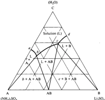
A large number of salt solubility diagrams have been studied, and a concluding example illustrates a case of double salt formation, shown in Fig. 11-22. Here, the compound L i²S 0⁴( N H⁴)²S 0⁴ forms.

The more symmetric ternary eutectic systems are of great general importance in metallurgy. Salt solubility systems are similarly central to the understanding of the evaporative recovery of salts from brines. The evaporation of brines, either from sea water or from dissolved natural salt deposits, constitutes our major source of most of such minerals.

FIG. 11-22. The H a O - L i a S O H N H ^ S O * system {near 2 5 ° C ) , illustrating double salt formation.

COMMENTARY AND NOTES, SECTION 1 413

COMMENTARY AND NOTES 11-CN-l Definitions of the Terms Component and Phase

The definitions given in Section 11-1 of the number of components of a system and of the number of phases present are adequate for the types of phase equilibria considered in this chapter. The subject is full of subtleties, however, and we now take a more careful look at what is meant by the terms component and phase.

Some explanation of the concept of a component was given in the introduction to Chapter 9. Briefly, a phase may contain a variety of molecular species but many of these will be in chemical equilibrium with each other and cannot therefore be varied independently. Pure liquid water has monomers, dimers and so on, and clusters, as well as H+ and OH~ ions; it is a one-component system because these species are all in equilibrium with each other. Water plus alcohol has water- alcohol clusters and so o n / but all compositions are fixed if the proportions of water-substance and alcohol-substance are given. The system is a two-component one.

The number of components is therefore the minimum number of formal com­

positions, such as concentrations, needed to define the state of a system at a given Τ and P. A complication begins to develop in the case of electrolyte solutions.

Aqueous sodium chloride is a two-component system; sodium and chloride ions cannot be varied independently because the system must remain electrically neutral. An aqueous mixture of NaCl and K N 0³ might be thought to constitute a three-component system. It is actually a special case of a four-component system.

The solution contains N a⁺, K⁺, Cl~, and N 0³~ ions; the four compositions are reduced by the electroneutrality requirement to three independent ones, plus water, for a total of four. Alternatively, the mole fraction of water, that of total salt, the Na+/K+ ratio, and the C 1^_/ N 0³- ratio define all possible compositions.

A second kind of problem is that the number of components may depend on whether or not a given chemical reaction is rapid within the time scale of the phase equilibrium studies. As mentioned in Section 9-1, the system hydrogen- nitrogen-ammonia consists of either two or three components according to whether or not chemical equilibrium is reached rapidly, ln dealing with freezing point diagrams, we took up briefly cases of compound formation. If such formation is very slow, so that the compound is not in equilibrium with the reactants that form it, then the compound must be treated as an additional component.

The reader can perhaps appreciate at this point why the phase rule often helps one decide just how many components are effectively present in a given system.

We have mentioned the preceding complications in order to give depth to the definition of component. The actual systems described in this chapter present no such problems.

We next consider the definition of the term phase. A phase is first of all a homo­

geneous portion of matter, by which we mean that its time-average properties do not vary discontinuously from one spot to another. A phase region must be large enough that random, thermal fluctuations are small, otherwise the operational definition would become impossible to apply. Adjacent phase regions are marked by an interface or discontinuity in properties. The derivation of the phase rule is based on the further requirement that the chemical potentials of all components

SPECIAL TOPICS

11-ST-l Two-Component Freezing Point Diagrams. Partial Miscibility

The freezing point diagrams so far considered have all been ones for systems in which the solid phases were entirely immiscible. The other extreme is that of complete miscibility in both liquid and solid phases. The appearance would be that of Fig. 11-23(a). We next imagine a progressive change in the properties of A and of Β such that the miscibility in the solid state gradually decreases and the miscibility gap moves upward. In Fig. 11-23(b) the miscibility gap has come close present are determined by the variables Ρ, T, and (C — 1) compositions. Neither these potentials nor any other molar thermodynamic properties ordinarily depend appreciably on the state of subdivision of the phase. Thus H²0 ( / ) and one piece of ice is a two-phase system; likewise H²0 ( / ) and two pieces of ice, and so on. The chemical potential of each piece of ice is the same and is independent of how many pieces are present.

A problem develops if the particles of a phase are so small that their chemical potential does depend appreciably on size owing to the surface energy contribution.

The Kelvin equation (8-43) gives the free energy of a small particle as a function of Τ and of particle radius r. The molar free energy also depends on total mechanical pressure; it is therefore a function of Ρ , Γ, and r. It is possible to derive a more general form of the phase rule which includes specific interfacial areas as state variables. It would apply, however, to the final equilibrium condition in which all condensed phases had collected into single individual regions. Thus the two pieces of ice in the preceding example should eventually become a single piece.

The mechanism would probably be through the dissolving of the smaller piece (its free energy being greater because of the smaller r) and growth of the larger piece.

This matter is not a trivial one. A precipitate of AgCl, for example, initially consists of a dispersion of particle sizes. Is, now, the measured solubility that of the smaller or of the larger crystals ? (It appears to be that of the smaller ones.) Such precipitates will usually age or equilibrate to what appears to be nearly the equilibrium solubility. In colloidal suspensions, however, the particles may be prevented from merging by interparticle repulsions (see Section 21-1) and m a y b e too insoluble to age by a dissolution-reprecipitation process. The system is then metastable in this respect, even though a range of particle size is present. How many phases are present? In the case of aqueous colloidal electrolytes, there is a concentration above which aggregates of 50 to 100 monomer units, called micelles, form. This critical micelle concentration is not as sharply defined as is a solubility limit, but almost so. D o micelles represent a new phase?

Questions such as these arise in the study of phase equilibria, and in difficult situations the phase rule itself may be used as the criterion for establishing the number of phases present. That is, if one knows the number of components in a system and can determine the number of degrees of freedom one defines the number of phases present.

SPECIAL TOPICS, SECTION 1 415

to the melting points of A and B, and the incipient immiscibility is reflected in the minimum of the solid solution-liquid solution composition curves.

In Fig. 11-23(c) the miscibility gap has impacted the freezing point curves and the system is now of the ^utectic type. Solution of composition x^E is in equilibrium at T^E with two solid phases. These are not pure A and B, but solid solutions of composition z^a and ζ^β. The letter ζ will be used to denote compositions of solid solutions and the Greek superscripts to indicate the type of phase. Thus an α phase is one that is rich in component A and a β phase one that is rich in component B.

Further diminution of the degree of miscibility leads to Fig. 11-23(d), essentially the same as Fig. 11-2.

Figure 11-23 also illustrates a succession o f boiling point diagrams for progressively less and less miscible liquids. W e n e e d only t o c h a n g e the labeling; L is replaced by vapor phase V, and solid solutions a a n d β by liquid solutions La and Lfi (note Fig. 9-19).

The Pb-Bi system is of the type of Fig. 11-23(c), as shown in Fig. 11-24. The cooling of a melt of composition (1) leads to a break at about 275°C as α phase begins to freeze out, and liquid and α phases would then vary in composition along their respective curves, with the latter increasing in amount. At about 175°C the system is entirely α phase [of composition (1)] and the cooling rate increases.

At about 50°C the system composition line crosses the solubility curve for α phase, and β phase begins to form. There is a break in the cooling curve at this point, but

F I G . 1 1 - 2 3 . Progression of appearance of a freezing point diagram with increasing degree of immiscibility of the solid phases.

F I G . 11-24. The P b - B i system.

F I G . 11-25. Development of peritectic type of freezing point diagram.

F I G . 11-26. The F e - A u system.

SPECIAL TOPICS, SECTION 1 417 not a marked one since the heat of separation into the two solid solutions is prob­

ably not large. Cooling curves for compositions between 37 and 9 7 % Bi are similar to those for a simple eutectic, except that the solid phases are α and β rather than the pure components.

The sequence of Fig. 11-23 is not the only possible one. If the melting points of the two components are fairly different and the miscibility gap is narrow, then the sequence of Fig. 11-25 may result. The diagram 11-25(b) is now of the peritectic type. At Γ^Ρ liquid of composition J C ^p is in equilibrium with solid solutions z^a and ζ^β; notice that the liquid composition lies outside of those of the two solid solutions rather than between them.

Iron and gold form a peritectic system, shown in Fig. 11-26, and some representa­

tive cooling curves may be considered. That for a system of composition (1) is analo­

gous to the cooling curve for Fig. 11-24 and need not be explained further. A system of composition (2) will show a break at about 1400°C, when α phase first forms. With continued cooling, liquid and α phase shift in composition along their respective lines, α phase increasing in amount. At 1170°C, or Γ^Ρ, the solution is now also in equilibrium with β phase, and there is a halt in the cooling curve while α and β phases (30 % Au and 65 % Au, respectively) crystallize out. The phase reaction is that of a peritectic system (see Section 11-3C), or L + a β. In this case L phase is used up first, and at the end of the halt the system consists of α and β phases only.

The cooling curve for a system of composition (3) is similar to that for (2) up to the halt. Phase α is now used up first in the phase reaction, however, so L and β phase remain at the end of the halt. With further cooling, L and β phase com­

positions shift along their respective curves, with β phase increasing in proportion, and at about 1150°C only β phase remains. Compositions to the right of the three- phase line give cooling curves similar to (1), but with β phase forming rather than a phase. Note that there is a slight minimum in the freezing point curve at (4), or 94 % Au. A liquid of this composition freezes to β phase of the same composition, and the cooling curve has the same appearance as that for a pure substance.

τ

A Β

F I G . 11-27. Partial miscibility in the liquid phases as well as in the solid phases.

Partial miscibility may occur in the liquid region to give a phase diagram such as illustrated in Fig. 11-27. The diagram is labeled, and one can work out the various cooling curves by following a system composition line through the various phase regions. A system of composition (1) would, for example, show one halt at 7\ while La phase converted to Le and α phase, and a second halt at TE while L0

phase converted to α and β phases.

Finally, no discussion of phase diagrams seems complete without a mention of the iron-carbon system. The diagram, shown in Fig. 11-28, illustrates yet another kind of partial miscibility—that between two different crystalline modifications of a solid phase. The stable crystalline form of pure iron below 910°C is body- centered cubic and is called α-iron. At 910°C α-iron changes to a face-centered type of crystal lattice called y-iron and then, at 1401 °C, there is a reversion back to a body-centered type of structure, now called δ-iron. The melting point of iron is 1535°C.

We explore the diagram by first dissolving some carbon in γ iron at about 1200°C, to give a solid solution called austenite of composition (1). On cooling to about 800°C α-iron containing some dissolved carbon begins to separate out. A eutectic- type three-phase line is reached at 700°C, at which point austenite phase of com­

position a is in equilibrium with α phase of composition b and F e3C (called cementite). Below 700°C the system consists of α-iron (with some dissolved carbon) and cementite.

This sequence corresponds to the heat treatment of steel. Iron with less than about 2 % carbon can be heated to the austenite single-phase region. It is then easily rolled or otherwise formed. On cooling, the separation into α-iron and cementite occurs, and the extreme hardness of cementite gives steel its strength.

The rate of cooling affects the particle size of the two-phase mixture and hence the mechanical properties o f the steel.

Consider next a system of composition (2) corresponding to about 2 . 5 % C.

FIG. 11-28. The F e - C system.

SPECIAL TOPICS, SECTION 2 419 On cooling of a molten iron-carbon solution, austenite phase of composition c begins to form, and with further cooling the liquid and solid solutions move in composition toward e and d, respectively, the proportion of the latter type of phase increasing. At 1125°C the eutectic is reached, and the system is now in equilibrium with F e³C ; during the halt austenite phase of composition d and F e³C crystallize out together. Below 1125°C the system consists of F e³C and austenite phase of composition moving along the da line. At 700°C the a-iron- austenite-Fe³C three-phase line is reached, and the further changes are as described earlier. An iron of this composition, unlike a steel, does not become a single phase until the melting point is reached. Such iron is called cast iron—it is not malleable when hot, but has valuable corrosion-resistant properties. If of composition close to the eutectic, its melting point is low enough to allow a fairly easy casting proce- dure.

The remaining small region in the upper left is of no great interest here. One can trace the details of its phase behavior by following system composition lines that pass through various portions of the region.

ll-ST-2 Partial Miscibility in Three-Component Systems

The water-phenol system was shown in Fig. 9-20(a); there is an upper consolute temperature of about 70°C and around room temperature the miscibility is rather limited. Acetone is fully miscible with water and with phenol separately and when it is added to a water-phenol two-phase system the effect is to increase the mutual solubility. The solubility behavior is shown in Fig. 11-29 for a temperature of about 30°C. The tie-lines connect pairs of mutually saturated solutions. Thus a system of overall composition (1) consists of liquid phases of compositions a and b and in amounts given by the lever principle. Addition of acetone moves the system com-

F I G . 11-29. The three-component miscibility gap. The H²Q-acetone-phenol system.

F I G . 11-30. The three-component miscibility gap in three dimensions.

position along the line drawn from point (1) to the acetone corner, the compositions of the two liquid phases being given by the ends of each successive tie-line. When the system composition reaches c only a single phase is present and further addition of acetone merely dilutes the liquid solution. The tie-lines themselves reach a vanishing point at d called the critical point.

The whole region of partial miscibility diminishes in size with increasing tem- perature, and a set of isothermal cross sections generates a helmet-shaped two- phase region in the three-dimensional phase diagram, as illustrated in Fig. 11-30.

The locus of successive critical points goes through the peak of the helmet (at 92°C, 59 % water and 29 % phenol), which is the critical temperature of the ternary system. Various cooling or dilution sequences may be traced out in the usual way by following the system composition line and, where it is in the two-phase region, using the ends of the tie-line through it to determine the compositions of the liquid phases present.

It must be remembered that while a tie-line is an isothermal line, there is no requirement that a set of lines such as for Fig. 11-29 be parallel. The ends of each successive line must be determined by individual experiment, and a set of tie-lines must be shown if the diagram is to be usable.

A number of types of miscibility gaps are possible for a ternary system, as illus- trated in Fig. 11-31. Figure 11-31(d) represents the case of partial miscibility in all three binary systems and Fig. 11-31(e) shows the result of a further decrease in miscibility, such as by lowering of the temperature. The three miscibility gaps have now merged to frame a central triangular region of three phase equilibrium.

Three-component freezing point diagrams with partial miscibility in the solid phases add partial miscibility regions to Fig. 11-15. A perspective drawing of such a model is shown in Fig. 11-32; the reader may enjoy working out the various phase regions. As with all models based on the prismatic coordinate scheme, each side shows a two-component phase diagram.

SPECIAL TOPICS, SECTION 2 421

F I G . 1 1 - 3 1 . Various types of three-component miscibility gaps.

FIG. 11-32. Three-component eutectic system with partial miscibility in the solid phases.

G E N E R A L R E F E R E N C E S

M A R S H , J. S. ( 1 9 3 5 ) . "Principles o f Phase Diagrams." McGraw-Hill, N e w York.

M A S I N G , G. ( 1 9 4 4 ) . "Ternary Systems" (translated by.B. A . Rogers). Dover, N e w York.

RICCI, J. E. ( 1 9 5 1 ) . "The Phase Rule and Heterogeneous Equilibrium." Van Nostrand-Reinhold, Princeton, N e w Jersey.

WETMORE, F. E. W . , A N D L E R O Y , D . J. ( 1 9 5 1 ) . "Principles o f Phase Equilibria." McGraw-Hill, N e w York.

C I T E D R E F E R E N C E

LIGHTFOOT, W . J . , A N D P R U T T O N , C . F . ( 1 9 4 7 ) . / . Amer. Chem. Soc. 69, 2 0 9 8 .

E X E R C I S E S

11-1 H o w many degrees o f freedom are present for the following systems: (a) ice plus a solution of alcohol a n d water; (b) a layer o f water saturated with phenol plus a layer o f phenol