Quantum Mechanics and Solid State Physics for Electric Engineers

(1)

Physics 3

Quantum Mechanics and Solid State Physics for Electric Engineers

Lecture Notes

A. S´ olyom and P. Richter Dept. Atomic Physics Faculty of Natural Sciences

Budapest University of Technology and Economics - BME

February 3, 2014

(2)

Introduction

The Master Course Physics 3 for Electrical Engineers is an introductory lecture to the fundamental concepts of modern physics. Here we present the basis of the disciplines Quantum Mechanics and Solid State Physics, all in one semester. As both of these topics are very broad we had to restrict the material presented to those areas which have the greatest practical importance. The unconventional concepts of these disciplines provide the physical basis for upt o dat engeneering. Therefore the method we are following does not requires complicated and subtle mathematics. We rely on disciplines well known for electrical engineers: the differential and integral calculus. Although during the semester we introduce the basics of operator calculus, to understand that part only elementary algebra is required.

The material in this book is organized in three distinct parts: Quantum Mechanics, Solid State Physics and the Appendices.

The first part deals with (non-relativistic) Quantum Mechanics which is the base of all of modern quantum physics. The phenomena, unexplainable in the frame of classical physics (see Chapter 2), required a re-evaluation of our knowledge of the world. In the beginning of the 20th century this lead to the development of quantum mechanics. In Chapter 3we introduce the stationarywave function (or state function) of a microscopic particle (e.g electron) and solve a handful of problems that help to understand the concepts. In Chapter4we discuss the problem of time dependent phenomena and introduce the time dependent Schr¨odinger equation. The most abstract chapter is Chapter5where the basics of the operator calculus and measurement theory is discussed. The next two chapters (Chapter 6 and Chapter 7) are devoted to the study of atoms with a central potential containing either a single or multiple electrons. This involves the quantum mechanics of the angular momentum, the hydrogen atom and elements inthe periodic table.

A discussion of formation of molecules follows (Chapter 8), which, leads to the under- standing of chemical bonds. In Chapter 9 the basis of statistical physics are introduced and the distribution functions of classical and quantum statistical physics are compared.

The final chapter in this part (Chapter 10) deals with the interaction between light and matter and the operation of lasers is also discussed.

(10)

The second part is about Solid State Physics. The first chapter of this part (Chapter 11) introduces the fundamental concepts. This mostly means crystal physics, although amorphous materials are also discussed briefly. Basic concepts like crystal lattice and crystal symmetries, primitive and other types of cells are introduced here. Chapter 12 presents experimental methods that are used for the determination of crystal structures.

Constituent atoms and molecules in crystals are vibrating around their equilibrium positions. These vibrations are the theme of Chapter 13, in which both classical and quantum mechanical models are discussed. Chapter 14introduces the concept of energy bands used in solid state physics. This is the chapter where questions about the electrical resistivity, the work function and contact potential of metals are discussed using semi-classical theories. This theme is examined from the viewpoint of quantum mechanics after introducing key concepts about movement of electrons in periodic structures in Chapter 15. While the previous chapters deal with electrons in conductors Chap- ter 16is about homogeneous and inhomogeneous semiconductors and their applications.

Superconductivity is also discussed. Chapter 17 is a short introduction to this topic with detailed examples for their practical application. Optical properties of solids are discussed next in Chapter 18. X-ray and visible light absorption and emission are the topics of this chapter. Chapter 19 discusses the magnetic properties of solids both from a phenomenological and microscopical point of view. Some of these can be explained using individual magnetic moments but quantum physics is required to explain for instance ferromagnetism. This part is closed with Chapter 20which is about the dielectric properties of crystals.

Important 0.0.1. To make it easier to recognize important statements, we mark them similar to this sentence¹.

Example 0.1. Problems with solutions are presented throughout the book marked similar to this.

The Appendix gives the reader an opportunity to see the details of the theories presented and understand the formulas more deeply.

1The PDF version of this document marks the important statements and the examples by putting them into colored boxes, however this feature is not available in the WEB version.

(11)

Chapter 1 Quantum Mechanics

(12)

Chapter 2 Experimental foundations

At the turn of the 20th century physics seemed to be a closed discipline¹. Everything seemed to fit perfectly. At the end of the 19th century all physical phenomena were described by one or more of the well known disciplines of Mechanics, Statistical Physics, Thermodynamics and Electrodynamics. This was the time when Maxwell’s electromagnetic theory was considered the theory of the “ether”, the elastic solid medium whose mechanical waves are the electromagnetic waves including light. The time when physicists tried to trace back all problems to problems of classical mechanics. There were of course some marginal unsolved problems left but almost all physicists agreed that physics in the 20th century will be “the physics of the 6th decimal place” (Michelson 1903). But some of the best physicists saw that this was not the case.

A closer examination shows that in fact many unsolved mysteries remained in physics at that time. It is now clear some of these could not have been incorporated into a classical theory at all. The problems that were considered unsolved at the beginning of the 20th century among others included the following

the velocity of light in vacuum is invariant Why is it independent of the frame of reference used? What happens between the ether and the bodies that move through it?

periodic system of elements What are the principles behind the periodic table? Why are the chemical behavior of elements in the same column similar?

spectra of atoms and molecules Why do we have discreet spectral lines? What is the reason behind the simple rules that govern the spectrum? Why do the splitting

1For instance the Munich physics professor Philipp von Jolly advised the young Max Planck against going into physics, saying, ”in this field, almost everything has been already discovered, and all that remains is to fill a few holes.” Planck replied that he did not wish to discover new things, but only to understand the known fundamentals of the field, and so began his studies in 1874 at the University of Munich. In spite of this remark Planck’s discovery of the energy quantum was the most important step towards Quantum Mechanics.

(13)

of the spectral lines in a magnetic field (the Zeeman effect) not follow the laws of the classical physics?

the problem of X-ray emission and absorption Why are X-rays emitted? How are they absorbed?

specific heat Why is the equipartition theorem true at high temperatures and why does it brake at low temperatures? Is it possible to have other statistical distribution functions than the Maxwell -Boltzmann function?

thermal radiation What formula describes the shape of the electromagnetic spectrum of an object at a given temperature? What is the physics behind it?

stability of the atoms According to electrodynamics an accelerating charge emits electromagnetic radiation and thereby loses energy. If we apply this principle to an electron in an atom then we find the electron should radiate all of its kinetic energy in about 10⁻⁸ sec, after that it should fall into the nucleus. But this is evidently not the case.

chemical bond Is chemistry based on physics? Can physics explain the chemical bond?

(external) photoelectric effect Why are the laws for an electron emission from a metal surface so complicated?

Compton effect Why does the frequency of the light change - when it is scattered by a free electron - the way it does?

radioactivity What causes the radioactive decay?

This list is not complete. Some of the problems (e.g. the invariance of the speed of light in vacuum) has lead to the development of the special then the general theory of relativity, others may only be explained using another new branch of physics: quantum mechanics. In this chapter we first discuss some of these phenomena that lead to the development of this new physics, some others will be addressed in later chapters.

2.1 Black-body radiation.

It was well known that if we heat an object to temperatures high enough it will emit visible light. The color of the light depends on the temperature of the material. The higher the temperature the bluer the color. We know that (visible) light is electromagnetic radiation with wavelengths in the 380 − 740nmrange. With suitable detectors we can verify that heated materials emit electromagnetic radiation not only in the visible part, but in every other part of the electromagnetic spectrum (infrared, ultraviolet).

(14)

This emission is characterized by the emission coefficient (also known as the black- body irradiance or emissive power) E(ν, T), which gives the energy a body emits at a given frequency at a given temperature in unit time. It has the dimension J/sec. The emission can be more exactly described by its derivative according to surface area and solid angle, called spectral radiance ε(ν, T) = ∂E(ν, T)

∂ν∂T which is the amount of energy emitted at a frequency νper unit surface area per unit time per unit solid angle per unit frequency. It has the dimension J·m⁻²·sec⁻¹·sr⁻¹·Hz⁻¹.

The color of a heated light emitting object is determined by the frequency dependence of ε(ν, T), (e.g. the frequency at which ε(ν, T) is maximum). As the temperature drops then the position of the maximum will shift toward the red then into the infra red range and the radio frequency range, but we can still detect electromagnetic radiation in the whole frequency range emitted by the material.

The frequency dependance of the intensity of electromagnetic waves on the wavelength frequency or energy over a specific portions of the electromagnetic spectrum is measured by spectrometers. See Appendix 22.1 for further information on spectrometers.

Materials not only emit but also absorb electromagnetic radiation. This absorption heats up the material. Therefore it is possible for an object to be in thermal equilibrium with electromagnetic radiation. The absorption of radiation can be characterized by the absorption coefficient a which tells us the ratio of the incoming radiation a body can absorb. The absorption coefficient is dimensionless, may depend on the frequency of the electromagnetic radiation and the temperature and must be between 0 and 1: 0≤a≤1.² Important 2.1.1. Every material at all temperatures absorbs and above0K also emits electromagnetic radiation in the whole frequency range. Some of the thermal energy of a body is converted into this electromagnetic radiation therefore it is called thermal radiation.

At the middle of the 19th century Kirchoff has found an interesting relationship between the absorption and emission of electromagnetic radiation (light) based on thermodynamics. Kirchoff deduced that the ratio ε(ν, T)

a(ν, T) must be the same for every material:

ε⁽¹⁾(ν, T)

a⁽¹⁾(ν, T) = ε⁽²⁾(ν, T) a⁽²⁾(ν, T) =...

otherwise a device coud be constructed that transfers heat from a body of lower temperature to a body of higher temperature without any external energy input, hereby violating the 3rd law of thermodynamics.

2The part of the radiation that is not absorbed may be reflected back or may pass through the material. The amount of this part is 1−a.

(15)

If we now introduce a hypothetical object called ablack-body³which absorbs all electromagnetic radiation falling on it independently of frequency and temperature, i.e. for which a ≡ 1 then we need to deal with the frequency and temperature dependence of ε(ν, T) only:

ε⁽¹⁾(ν, T)

a⁽¹⁾(ν, T) = ε⁽²⁾(ν, T)

a⁽²⁾(ν, T) =...=ε(ν, T) (2.1.1) Black-bodies do not exist in nature. But some materials with high absorption can be considered very close to this ideal black-body. Graphite, soot and lamp black⁴ have an absorption coefficient a ≥ 0.95. NASA⁵ has developed a more modern ultra absorbent material coated with carbon nanotubes which absorbs 99.5 % of the incoming UV and visible light and 98 % of the longer wavelengths, with an average a= 0.99. Such coatings can be used for instance for stealth aeroplanes.

The classical model of a black-body is a cavity in a rigid opaque body with rough absorbing walls like the one in Fig 2.1. A small hole in thewall allows a small part of the radiation exit that allows measurement of the internal radiation Such objects are fabricated by some companies and may be bought. They are certified in a given frequency range to behave like ideal black-bodies.

Because the absorption of a black-body is the largest absorption coefficient possible (a = 1), its emission coefficient is larger than for any other object. This means that a given temperature the black-body emits the most intensive radiation. It follows that for instance if we compare the emission of various objects we find that at temperatures when the maximum of the emission is in the visible range then black-bodies are the brightest objects

It was found that

Important 2.1.2. for black-bodies in thermal equilibrium with the electromagnetic radiation the product of the absolute temperature T and of the wavelength λ_max where the emission per unit wavelength has its maximum is constant (peak wavelength):

λ_max·T = 2.8977721(26)·10⁻³K m (2.1.2) This is Wien’s displacement law.

3Sometimes written as black body or blackbody.

4Also known as carbon black, furnace black or thermal black is a form of amorphous carbon that has a high surface-area-to-volume ratio, although its surface-area-to-volume ratio is low compared to that of activated carbon. It is dissimilar to soot in its much higher surface-area-to-volume ratio and significantly lower (negligible and non-bioavailable) PAH (polycyclic aromatic hydrocarbon) content. Its most common use is a pigment and reinforcing phase in automobile tires.

5NASA is an acronym for the agency National Aeronautics and Space Administration of the United States government that is responsible for the nation’s civilian space program and for aeronautics and aerospace research.

(16)

Figure 2.1: A model of a black-body is the hole of a cavity in a rigid opaque body. All incoming electromagnetic radiation is absorbed by the rough inner surface of the cavity in consecutive steps even when a <1 for the material of the body as there is little chance for any reflected radiation to exit again through the hole.

Example 2.1. The effective temperature of the Sun is 5778 K. What is the value of λ_max for the Sun? Solution

λmax= 2.90·10⁻³/5778 = 5.02·10⁻⁷m= 502nm

This corresponds to the wavelength of green light near the peak sensitivity of the human eye.

Example 2.2. According to theory, approximately a second after its formation the Uni- verse was a near-ideal black-body in thermal equilibrium at a temperature above 10¹⁰K. The temperature decreased as the Universe expanded and the matter and radiation in it cooled. The cosmic microwave Background radiation observed today is ”the most perfect black-body ever measured in nature” as it has an anisotropy less than 1 part per 100,000. Now, some 15 billion years after the Big Bang the peak of the observed cosmic Background radiation is at 1.07mm. What is the temperature of the cosmos? Solution

T = 2.898 10⁻³/λ_max= 2.7K

The Stefan-Boltzmann law states that the total energy emitted (λ∈[0,∞]) by a black- body per unit surface area is proportional to the 4th power of the absolute temperature:

P_A =σ T⁴ (2.1.3)

(17)

where σ = 5.670373(21)·10⁻⁸W m⁻²K⁻⁴ is the Stefan-–Boltzmann constant

Example 2.3. A human body also radiates energy. Calculate the total energy needs for an adult to keep the body temperature constant. Because the mid- and far-infrared emis- sivity of skin and most clothing is near unity we may approximate the human body with a black-body. The average total skin area of an adult human being is about 2m², and in an ambient temperature of 20ôC the temperature of the bare skin is about 33ôC, while under the clothing it is about 28ôC .

Solution From Wien’s law (equations (2.1.2)) the peak wavelength of the thermal radiation of a naked human body is is about 9.5µm⁶. To calculate the energy needed to keep the temperature of the body constant can be obtained from the Stefan-Boltzmann law (2.1.3). The radiated power is the difference between the power absorbed from the environment (which is also considered a black-body) and the one emitted by the body:

P_body =P_absorption− P_emission = 4π σ(T_environ⁴ −T_body⁴ )A

=−95.10W

The total energy requirement for a whole day therefore is E =−P_body·24·3600 = 8.216M J = 1965kcal

Example 2.4. Let us model the Earth with a perfect spherical black-body without an atmosphere! Determine the effectiveor average surface temperature if the solar constant I_o, i.e. the amount of incoming solar electromagnetic radiation per unit area – that is incident on a plane perpendicular to the rays, at a distance of one astronomical unit (AU) (roughly the mean distance from the Sun to the Earth) – was 1361kW/m²! Solution In the stationary state the “model ‘Earth” absorbs the same amount of energy from the Sun as it emits. The Earth-Sun distance is so large that the rays of sunshine are almost parallel when they reach us. Half of the Earth surface is illuminated all the time by the Sun. The total energy absorbed by the Earth as a black-body, therefore equals to the solar constant multiplied by the cross section of the Earth perpendicular to the Earth-Sun direction⁷ and by the duration ∆t

Etot,absorbed =R²π·I_o·∆t

6Therefore thermal imaging devices are tuned to be most sensitive in the 7–14 micron range. But the human body emits at much larger wavelengths too. New imaging devices used in some border stations or airports use wavelengths in the 1 cm–1 mm (terrahertz) range. These are most suited to detect people smuggled in trucks.

7The sunlight I is perpendicular to the surface only at the point nearest to the Sun. Let us take a cross section of the sunlight with an area ofAat this point. At aθangle to the direction of the Sun this part of the sunlight hits a larger areaA⁰=A·cosΘ, but only the component perpendicular to the surface is absorbed, which isI⁰=I_o/cosθ. The total absorbed radiation flux thereforeP =A·cosΘ·I/cosθ=IA is the same at every point of the illuminated surface with a perpendicular surface area of A.

(18)

If the surface temperature is T then the total radiated energy from the Earth according to the Stefan-Boltzmann law is

E_tot,rad = 4π R²σ T⁴·∆t

In a stationary state these two energies must be equal:

Etot,absorbed=E_tot,rad from which

T = ⁴ r Io

4σ = 278.3K = 5.3^oC

The real effective temperature of the Earth is higher, because of the atmosphere.

Example 2.5. The albedoor reflection coefficient of the Earth is 0.3. This means that 30% of the solar radiation that hits the planet gets scattered back into space without absorption.

a) In the previous example what would be the temperature if the absorption coefficient of the Earth was a= 0.7 instead of 1?

b) In climate calculations it is sometimes assumed that regardless to reflection the Earth still emits like a black-body (this contradicts Kirchoff ’s law). What would the temperature be with this assumption?

Solution a)

If a= 0.7 then the absorbed energy isI_a =I_oa, a times as much as above, and according to Kirchoff ’s law the emission must be lower by the same factor, i.e. E_tot,rad⁰ = a E_tot,rad, therefore the temperature is the same as was in the previous example, namely 5.3^oC.

b)

In this case

Etot,absorbed = 0.3R²π·I_o·∆tE_tot,rad = 4π R²σ T⁴·∆t and the temperature

T = ⁴ r0.7I_o

4σ = 254.58K =−18.58^oC

If a black-body can be fabricated (See Fig. 2.1), then ε(ν, T) can be measured.

The resulting spectrum of such a measurement on materials, which at least in a limited frequency (wavelength) range, absorb almost all of the electromagnetic radiation look like

(19)

Figure 2.2: Calculated black-body emission curves and λ_max values.

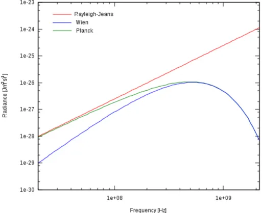
the curves shown in Fig 2.2. Knowing the spectrum of a black-body in equilibrium with the electromagnetic radiation makes it possible to determine its temperature. Although real objects just approximate black-bodies the knowledge of the black-body spectrum and the spectra of the objects still gives a fairly good opportunity to remotely measure their temperatures even when the condition of thermal equilibrium does not hold. An example that the laws of black-body radiation can be applied with a good approximation is shown in Fig. 2.3 where the emission curve of our Sun, measured both above and below the atmosphere is shown⁸ together with the calculated spectrum of a black-body of temperature 5250 K. In Fig. 2.3 the calculated black-body spectrum reflects our present knowledge. Previous attempts could describe the radiation only at part of the spectrum. The two most famous are: the formula of Lord Rayleigh and Sir James Jeans, based on the equipartition theorem and Wien’s approximation. The Rayleigh-Jeans law describes only the long wavelength (i.e. low frequency) part of the spectrum:

ε(λ, T) = 2ckT

λ⁴ (2.1.4a)

or with the frequency

ε(ν, T) = 2kT ν²

c² (2.1.4b)

8At sea level 3% of the radiation is ultraviolet, 44 % is in the visible range and 53 % is in the infrared.

The gaps in the spectrum measured at sea level (red) are caused by greenhouse gases like water vapor and carbon dioxide. Water vapor has a larger absorption than CO2.

(20)

– and tends to infinity as the wavelength decreases (or the frequency increases). This is called the“ultraviolet catastrophe”. For short wavelengths (i.e. high frequencies)Wien’s approximation combines Wien’s displacement law with the Stefan-Boltzmann law. It contains two empirical constants⁹ C₁ and C₂:

ε(λ, T) = C1

λ⁵e⁻^C^{λ T}²^{h c} (2.1.5a) ε(ν, T) = C₁ν³

c⁴ e⁻^C^{c T}²^ν (2.1.5b)

– which tends to infinity as the wavelength increases (or the frequency decreases). This is called the“infrared catastrophe.

Max Planck found an interpolation formula, which used empirical constants, in late 1900 and published it in 1901. Later he discovered the derivation of the same formula for a black-body modeled as a cavity whose walls were in thermal equilibrium with the electromagnetic radiation inside the cavity.

ε(λ, T) = 2hc² λ⁵

1

e^hc/(λk^B^T⁾−1ε(ν, T) = 2hν³ c²

1

e^hν/(k^B^T⁾−1 (2.1.6a) But this derivation required that the energy of the material of the wall of the cavity and of the electromagnetic field may only change in discreet values of ε =hν, where

h≈6.62·10⁻³⁴ J (2.1.7)

is the Planck constant¹⁰, which we now call the quantum of energy. This was a sig- nificant leap for physics because every physicist (even Planck himself) were sure that electromagnetic energy is a continuous quantity. He tried for some months to get rid of this quantum in his derivation but without success.

In Fig. 2.4 we visually compare the three laws for a black-body of temperature 0.008 K.

Important 2.1.3. The concept of the existence of an energy quantum cannot be incorporated in classical physics. This was the first and most important step of the development of quantum mechanics.

9Comparing Wien’s with the correct Planck’s formula in the limits we can determine these: C1≡2hc² and C2≡ _k^hc

10The Planck constantB hwas introduced first in 1899.

(21)

2.2 Photoelectric effect

In 1887 Heinrich Hertz observed that that electrodes illuminated with ultraviolet light create electric sparks easily. It was established later that metal surfaces illuminated by light of suitable frequencies emit electrons. This is called the photoelectric effect.

The experimental setup is shown in Fig. 2.5. Three electrodes (cathode (C), grid (G) and anode (A)) are sealed inside a vacuum tube¹¹. When light illuminates the cathode electrons are emitted from it. These electrons are then accelerated toward the anode by the U voltage producing a current which is measured by an ammeter. The grid electrode is used to measure the kinetic energy of the electrons emitted. When the voltage UG

between the grid electrode and the cathode is such that the i current disappears then the kinetic energy of the electrons is e·U_g. It seems easy to explain this behavior by (classical) electrodynamics but the predictions of such a classical model disagree with the measured characteristics of the emitted electron current, which are summarized in Fig. 2.6.

1. Electron emission occurs less than 1µsecafter the illumination starts independent of the light intensity. Classical theory predicts a light intensity dependent emission time.

2. increasing the light intensity the current increases linearly, therefore all emitted electrons have the same kinetic energy independent of the light intensity. Classical theory predicts a non-linear relationship.

3. No current is observed if the frequency of the light is less than a threshold frequency, which depends on the metal of the cathode. Classical theory predicts that emission is independent of the frequency.

4. The kinetic energy of the electrons depends only on the frequency of the light but independent of the light intensity. Classical theory predicts that kinetic energy depends on the light intensity.

It was Albert Einstein who explained the measured characteristics of the photoelectric effect¹². He used Planck’s idea of the energy quantum and assumed that the energy of

11A.k.a. electron tube (in North America),thermionic valve, tube, or valve. It is a device controlling electric current through a vacuum in a sealed container for switching and amplification of electrical signals. Before transistors and integrated circuits were developed these vacuum tubes were used in all electronic equipments. In those devices the cathode is heated to a high temperature and produces electrons by the thermionic effect (see Section 14.4). The electrons are accelerated by the voltage between the anode and cathode. One or more grids could also be placed inside the tube which may control the current. In the photoelectric experiment the cathode needs not to be heated.

12Contrary to popular belief Einstein received the Nobel prize for the explanation of the photoelectric effect and not for his theory of relativity.

(22)

the light is also quantized, namely that the light consists of “particles” he called photons that have an energy of h ν. The intensity of the light is the number of photons in it, while the energy is the photon energy multiplied by the photon number. Therefore when we illuminate a surface with light of frequency ν we bombard it with photons of energy h ν. An electron is emitted from the material only when an incoming photon, that has enough energy to overcome the electron binding energy W, called thework function¹³.

h ν = 1

2m_ev²+W (2.2.1)

where W is the work function, v is the velocity and, m_e = 9.1·10⁻³¹kg is the mass of the electron.

Important 2.2.1. In quantum mechanics the energy is usually measured in electronvolts (eV). 1 eV is the energy an electron obtains if accelerated through 1 V. Because∆E =e U, whereU is the potential difference measured in volts andeis the elementary charge, which is ≈1.60·10⁻¹⁹C :

1eV ≈1.6·10⁻¹⁹J

Units of milli-, kilo-, mega-, giga-, tera- or peta- electronvolts (meV, keV, MeV, GeV, TeV and PeV respectively) are also used in practice¹⁴.

The probability of multiple “collisions” is negligible at normal light intensities, therefore if the frequency is lower than a threshold frequency (i.e. the photon energy is smaller than the work function) no electrons are emitted. As the emission of an electron occurs immediately after the arrival of a photon with a frequency above the threshold the intensity of the light does not matter. Furthermore increasing the light intensity only increases the number of photon collisions and not the kinetic energy of the electrons, therefore the current, which depends on the number and velocity of the electrons, will be proportional with the intensity, as the velocity (kinetic energy) of the electrons depends only on the frequency.

Important 2.2.2. The photoelectric effect can only be explained by assuming the existence of photons: the discreet energy quanta of electromagnetic radiation. These photons behave like particles. They may collide with electrons for instance. Light (or electromagnetic radiation of any frequency) is emitted and absorbed in quanta. Therefore electromagnetic radiation must be a corpuscular phenomena. But diffraction and interference experiments can only be explained by assuming that light is a wave. This is the so called particle-wave duality of the electromagnetic radiation.

13See also section 14.4.

14The velocity of an electron with a kinetic energy of 1 eV calculated using classical Newtonian (non- relativistic) mechanics isv=

r2·e me

= 1.5·10⁶ m/s= 0.015·c, wherec≈3·10⁸ is the velocity of light in vacuum. Using the correct relativistic formula, which ensures that the velocity of the electron never reachesc no matter the kinetic energy of the electron yields the lower value ofv= 5.93·10⁵m/s

(23)

Example 2.6. Determine the work function of potassium in electronvolts knowing that when illuminated by a light with a wavelength of λ = 560nm it emits electrons with a velocity of 190km/s! Solution From equation (2.2.1)

W =h ν−1

2mev² =h c λ −1

2mev² = 3.38·10⁻¹⁹J = 2.11eV

Example 2.7. Determine the maximum speed of a photoelectron emitted from a chromium surface when illuminated with light of a wavelength of 180 nm, from knowing that at a wavelength of 150nm the maximum photoelectron energy is 3.92eV? How large is the work function? (m_e = 9.1.10⁻³¹kg)Solution Letλ₁ = 1.8·10⁻⁷m andλ₂ = 1.5·10⁻⁷m and the maximum photoelectron kinetic energy at λ2 Ekin(λ2) = 3.92eV. From equation (2.2.1) and using ν =c/λ the work function can be determined:

W =h c

λ₂ − E_kin(λ₂) = 6.96·10⁻¹⁹J = 4.35eV Therefore the maximum velocity at λ₁:

v(λ₁) = s

2 m_e

h c

λ₁ −W

= 945,970m/s

2.3 Compton effect

By the early 20th century, researchers found that when X-rays of a known wavelength interact with electrons, the X-rays are scattered through an angle θ and emerge at a different wavelength related to θ. Although classical electromagnetism predicted that the wavelength of scattered rays should be equal to the initial wavelength, multiple experiments found that the wavelength of the scattered rays was longer (corresponding to lower energy) than the initial wavelength. That is, regardless of light intensity inelastic scattering always occurs when the frequency of the light is high enough (so that photon energies are in the range corresponding to the electron rest mass: m_ec² = 511keV) and the scattering angle is not zero.

According to classical electrodynamics the incident harmonic electromagnetic wave accelerates the charged particle which, in turn, then emits an electromagnetic radiation of the same frequency as of the incident wave. As long as the velocity of the particle is much smaller than the speed of light in vacuum the magnetic component of the electromagnetic wave does not affect the motion of the particle. The resulting, scattered wave therefore will have the same frequency as the original one¹⁵.

15Classically, the electric field in light of sufficient intensity may accelerate a charged particle to relativistic speeds, which will cause radiation-pressure recoil and an associated Doppler shift of the scattered light, but the effect would become arbitrarily small at sufficiently low light intensities regardless of wavelength.

(24)

Light scattering on free electrons (or on other charged particles) can be elastic or inelastic. Elastic scattering in which neither the particle kinetic energy, nor the frequency of the light changes is called Thomson scattering. Inelastic scattering in which both the energy and momentum of the electron (or any charged particle) and the frequency of the light changes – the frequency of the light always decreases – is calledCompton scattering, and the frequency shift of the light is theCompton effect. Thomson scattering is the low energy limit of Compton scattering.

Assuming light consists of photons which can collide with electrons we can easily explain the observed behavior, by applying the (relativistic) energy and momentum conservation laws¹⁶. Details of the derivation are in Appendix 22.3. The result is

λ⁰−λ= h

m_ec(1−cosθ), (2.3.1)

where λ is the initial wavelength, λ⁰ is the wavelength after scattering, h is the Planck constant, m_e is the electron rest mass, c is the speed of light, and θ is the scattering angle. The quantity

h

mec = 2.43·10⁻¹²m (2.3.2)

is known as the Compton wavelength of the electron. The amount ∆λ = λ⁰ −λ the wavelength changes by is called the Compton shift. It is between zero (for θ = 0^o) and twice the Compton wavelength of the electron (for θ= 180⁰).

Important 2.3.1. The Compton effect is another phenomenon that can only be explained by assuming the existence of photons.

Example 2.8. Calculate the scattering angle and the energy transferred to the electron compared to the energy of the incoming photon in a Compton effect, if at wavelength λ = 0.01nm ∆λ = 0.0024nm. Solution From (2.3.2) the Compton angle is

cos θ = 1− m_ec∆λ

h = 0.989 ⇒ θ= 8.445^o The energy transferred to the electron is

E_e =h c 1

λ − 1 λ⁰

=h c 1

λ − 1 λ+ ∆λ

= 3.84·10⁻¹⁵J = 24keV

The energy of the incoming photon according to the theory of relativity is E_ph =h ν=h c /λ= 1.99·10⁻¹⁴J, i.e E_e

E_ph = 0.19.

16Because photons are characterized by their frequency the photon after the scattering is not the same particle as the photon before the scattering.

(25)

Example 2.9. What will be the momentum of the Compton electron if forλ = 0.005nm the photon scattering angle is 90^o? Solution If the Compton angle is 90^o then cos θ = 0 and

λ⁰ =λ+ h

m_ec = 7.426·10⁻¹²m= 0.007426nm

Because of the momentum conservation the total momentum of the electron after the collision equals to the total momentum difference between the incoming and outgoing photons. The photon momentum and energy is connected by the formula p_photon =E_photon/c=h ν/c. Therefore

∆p_e = h ν

c − h ν⁰ c = h

λ − h

λ⁰ = 4.33·10⁻²³kg m s⁻¹

(26)

Figure 2.3: Emission spectrum of the Sun. When measured above the atmosphere (yel- low) the spectrum resembles that of a black-body whose temperature is 5250 K. At sea (ground) level the spectrum (red) is distorted because gases in the atmosphere absorb radiation at some wavelengths.

(27)

Figure 2.4: Comparison of the Rayleigh-Jeans, Wien and Planck formulas for a black body of temperature 8 mK.

Figure 2.5: Experimental setup of the measurement of the photoelectric effect. For description see the main text.

(28)

Figure 2.6: The photoelectric effect. a) current vs emission time, b) current vs light intensity, c) kinetic energy vs frequency curve for K and Cu, d) The kinetic energy of the electrons (E_kin

e = U_G) is independent of the light intensity. It only depends on the frequency and a material specific W constant.

(29)

Chapter 3 Stationary states

3.1 Stationary States

One of the phenomena, mentioned above, which could not be explained by classical physics, is the stability of atoms, molecules and even the stability of the atomic nucleus.

According to classical electromagnetic theory¹ there can be no stable equilibrium in a system of charged particles if no other interaction is present. As we now know all mechanical interactions between macroscopic bodies are in fact electrostatic interactions of the outermost atoms of the interacting objects, so this means that the system of charged particles must be in continuous motion, otherwise no stable macroscopic or microscopic bodies could exist. On the other hand if moving charged particles are confined into a finite volume of space they cannot move with constant velocity, therefore must accelerate. But, according to the classical theory of electromagnetism, all accelerating charges emit electromagnetic radiation, which means energy loss. Therefore neither the atoms, nor the molecules could be stable. The calculation of the energy loss rate of the single electron in a hydrogen atom for instance yields that the time during which all kinetic energy of the electron is lost is less than 10⁻⁸ sec. As the universe is older than that clearly something must be wrong with this picture.

The discrepancy between the theoretical predictions and the experiments can be resolved if we assume, that there exist discreet stationary states of a system of charged particles in which they do not emit electromagnetic radiation contrary to the prediction of classical (macroscopic) electromagnetic theory. This was exactly what Bohr proposed to explain the observed line spectra of atoms.

Important 3.1.1. The existence of stationary electronic states does not mean that the laws of electrodynamics are invalid for electrons. Neither do they mean that there ex- ists a special kind of “quantum mechanical interaction” between particles. There is no

1which itself was only discovered in the second half of the 19th century.

(30)

such thing. There are only four fundamental interactions (sometimes called fundamental forces), namely electromagnetism, strong interaction (or strong nuclear force), weak interaction (or weak nuclear force) and gravitation.

All of the “forces” we encounter in quantum mechanics are electromagnetic forces.

What must be modified is the classical concept of the electron being a classical charged mass point.

So the fact electrons in stationary states in an atom do not emit electromagnetic radiation means that – contrary to classical physics – they do not accelerate, i.e. they are not orbiting the atom in a classical way.

But when charged particles change their state as a result of an interaction with their environment then during the transition from one stationary state to an other one they either emit or absorb energy. Energy may be absorbed for instance in a collision with a photon of suitable frequency, and emitted in the form of a photon of the same frequency.

This picture can explain for instance the absorption and emission spectra of atoms.

We will denote stationary (bound) atomic or electronic state “A” by |Ai. The energy of the electron in state |Ai will be E(|Ai). As we will see the energy of electrons in stationary states in atoms can have only discreet values E(|Ai),E(|Bi), etc. An atom originally in the discreet stationary state |Aimay absorb a photon and change its state to another, higher energy discreet state |Bi if and only if the following criterion is met:

E(|Bi)− E(|Ai) = ∆E (|Ai → |Bi) =h ν

In the opposite process the atom goes from the higher energy state to the lower energy one with an emission of a photon with same ν frequency:

∆E(|Bi → |Ai) = −h ν

The discreet nature of atomic energies can be observed by experiments in which no photons are involved at all.

The most famous such experiment was performed byJames Franck and Gustav Luis Hertz in 1914². The schematic of theFrank-Hertz experiment can be seen in Fig. 3.1.

What would we expect from this experiment if we assume that atomic stationary states have discreet (quantized) energy values (called energy levels)? For simplicity let us assume mercury atoms have two possible stationary states with discreet energies (energy levels) with an ∆E energy difference between them.

Until the kinetic energy of the emitted and subsequently accelerated electrons is smaller than ∆E no interaction is possible with the Hg atoms, because the atoms can

2They were awarded the Nobel Prize in 1925 for this work.

(31)

Figure 3.1: Experimental setup of the Franck-Hertz experiment. Electrons are generated by a heated cathode in a glass vacuum tube filled with low pressure mercury gas. They are accelerated by the variable voltage between the cathode and the grid. The anode is held at a slightly negative potential relative to the grid, so that only the electrons with suitable kinetic energy may reach it. The accelerating voltage is varied and the I current is measured.

only absorb ∆E energy not less and not more. Therefore only elastic electron–atom collisions are possible, which do not change the kinetic energy of the electrons, only randomize the direction of their velocity. This means that the current will increase steadily after the acceleration voltage is higher than the grid voltage 0.5 V.

When the kinetic energy of the electrons reaches ∆E the current should drop almost to zero, because now inelastic scattering leading to kinetic energy loss may also occur³.

A further increase of the acceleration voltage will lead to the increase of the current again, because electrons can only loose ∆E of their kinetic energy in a collision and not more. Until the remaining kinetic energy is smaller than ∆E no further inelastic collision may occur. However when the average electron kinetic energy reaches 2 ∆E the current drops again, as electrons now have enough kinetic energy to participate in two consecutive inelastic collisions⁴. And this periodic increase and decrease of the current

3The current will not drop exactly to zero because of two reasons. First there will be electrons that travel from the cathode to the grid without any collisions and, second, some percentage of the electrons will still collide elastically with the atoms, as not all electrons will have the same amount of kinetic energy.

4The minimum current will be higher than in the previous case, because the probability of two

(32)

will repeat at 3 ∆E, 4 ∆E, etc, i.e. at every multiple of ∆E.

In Fig. 3.2 part of the results of the original experiment, which clearly displays the expected behavior is shown. From the figure we can determine that for mercury

Figure 3.2: Accelerating voltage vs. anode current. The current is displayed in arbitrary units (a.u.)

∆E = 4.9eV

This periodic current may be observed up to at least 100 volts. The same experiment with neon gas gives ∆E_neon = 19 eV.

Important 3.1.2. The Franck-Hertz experiment proves that stationary atomic energy values are discreet. Clearly the quantized nature of some physical quantities is a basic law of nature.

Example 3.1. The ground state and the first excited state (the stationary states with the smallest and the next lowest energy) in a hydrogen atom have an energy of E₀ =

−13.6eV and E₁ =−3.4eV respectively relative to the energy of the free electron. What

consecutive inelastic collisions is smaller than the probability of a single one.

(33)

is the frequency of the photon that, when absorbed, can excite the electron from the ground state to the first excited state? What will be the frequency of a photon emitted during the E₁ → E₀ transition? Solution For a photon to be absorbed the photon energy must equal to the energy difference of the two states in question:

h ν =E1 − E0 = 10.2eV = 1.634·10⁻¹⁸J ⇒ ν= 2.47·10⁺¹⁵Hz

The frequency of the photon emitted in the reverse transition must be the same as that of the absorbed photon.

3.2 Wave-particle duality

In previous sections we encountered the dual nature the electromagnetic waves. In some cases (e.g. diffraction and interference) they behave like classical waves, in other cases (e.g. Compton effect, photoelectric effect) like classical particles (photons). We also saw that stationary states of physical systems may (and usually do) have discreet energy values. A valid question therefore whether particles (e.g. electrons) may exhibit wave-like behavior too.

This possibility first appeared in an 1924 paper of the French physicist and Nobel laureate Louis de Broglie. According to the de Broglie hypotheses any moving particle or object had an associated wave, with a wavelength determined by its momentum p:

λ= h

p (3.2.1a)

With the introduction of the wave number k = 2π

λ (3.2.1b)

this formula can be written as

p= h

λ =~k (3.2.1c)

where

~≡ h 2π

is the reduced Planck constant⁵. We can define the frequency of this wave by the energy E as we did for photons:

E =h ν =~ω (= p² 2me

= ~²k² 2me

) (3.2.1d)

5Pronounced “h-bar”. It is also known asDirac’s constant.

(34)

If the de Broglie hypothesis is true, then diffraction and interference patterns should be observable in experiments involving only electrons and other particles. Indeedelectron diffraction experiments performed on thin metal foils clearly show these patterns. In Figure 3.3 for instance we can compare X-ray and electron diffraction measurements performed on the same aluminum foil. Both the electromagnetic X-rays and low energy electrons have wavelengths of the same magnitude.

Example 3.2. Determine the wavelength of an electron that is accelerated through a voltage U. What magnitude of voltage must be used to have a wavelength comparable to atomic distances around 0.05-10 nm in solids? Solution The kinetic energy of an electron of momentum p is E_kin = p²

2m_e. If the electron is accelerated through aU voltageE_kin =e U (e is the elementary charge). The corresponding momentum is

p=p

2m_ee U The de Broglie wavelength

λ= h

p = h

√2mee U Therefore the accelerating voltage for λ is

U = h² 2m_ee λ²

For wavelengths 0.05nm and 10nm the required voltages are:

U(0.05nm) = 601.7V and U(10nm) = 0.015V

The Double-slit experiment with light and with electrons

The famous double-slit experiment illustrates best the difference between wave-like and particle-like behavior. The original experiment used light, but the double-slit experiment has been replicated with electrons (in 1961), atoms, and even entire molecules (in 1999).

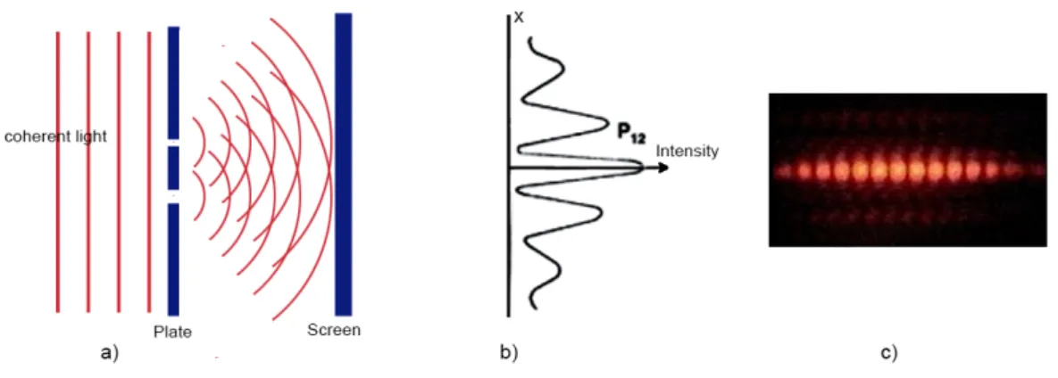
The principle of the original experiment is as follows: a light source producing coherent plane waves⁶ illuminates a thin plate pierced by two parallel slits. The light passing thorough the slits then hits a screen. Because the light is (or more exactly as we have seen before: may behave like) a wave we expect an interference pattern on the screen⁷. See Fig. 3.4.

6Light is said to becoherentif it can be split into two or more parts whose relative phases, when united again after traveling paths of different lengths does not change so the interference patterns produced

(35)

Figure 3.3: Comparison of X–ray and electron diffraction experiments. a) X-ray diffraction on a thin aluminum foil. b) an electron beam directed through the same foil gave this diffraction picture.

However when one of the slit is covered and light may only travel through the other one the interference vanishes⁸ (Fig. 3.5).

These experiments conform to the expected behavior from a wave. If we put a pho- todetector (photomultiplier, CCD or CMOS sensor, etc) near one of the slits we either detect a photon or nothing at all again since the energy in electromagnetic waves are in (particle like) photons. This makes it possible to determine which one of the slits the ac- tual photon went through. Unexpectedly however, if we do this, the interference pattern vanishes and the screen shows the sum of two overlapping intensity peaks, corresponding to the two slits (See Fig. 3.6. ) Therefore it may seem logical that the wave and particle properties of the light (or any particle whatsoever) are complementary: both cannot be observed at the same time.

are stationary in time. Such light may be produced e.g. a monochromatic laser as a light source.

7The same interference pattern forms regardless of the light intensity only the required measurement times vary. In 1909 this was proved in an experiment where such low light intensities were used that only a single photon was present in the device at one time. In this case the interference pattern is built-up the same way as is shown in Fig. 3.7for electrons.

8You can still observe adiffraction pattern on c).

(36)

Figure 3.4: The double slit experiment 1. a) schematics with both slits open, b) intensity measured on the screen, c) observable interference pattern

Figure 3.5: The double slit experiment 2. a) schematics with one slit covered, b) intensity measured on the screen, c) observable interference pattern

(37)

Figure 3.6: The double slit experiment 3. a) setup with a photon detector, b) intensities of the two independent slits, c) the intensity on the screen is the sum of the intensities of the two slits

Important 3.2.1. The wave and particle like behavior of either particles and waves are both present simultaneously always. Which behavior manifests itself depends on the properties of the object (e.g. photon or electron) and on the parameters of the experiment.

The measured intensity of a wave is the square of the absolute value of the instantaneous complex amplitude A(x, t) = A₀eⁱ^{(ω t−k r)}. The difference between the interference pattern in Fig. 3.4 and the intensity curve in Fig. 3.6 is that in the first case, when the wave–like property of the photons is dominant, the resulting intensity is the square of the sum of the instantaneous amplitudes:

I(x, t) = (A₁(x, t) +A₂(x, t))² =A²₁+A²₂+ 2A₁· A₂

The third term in this expression is theinterference term. It may be positive or negative depending on the phase difference between A₁ and A₂.

When the particle–like property of the photons⁹ is dominant the resulting intensity is the sum of the intensities from the slits:

I(x, t) = I₁(x, t) +I₂(x, t) =A₁(x, t)² +A₂(x, t)² The difference being the missing interference term in the second case.

At first thought it may seem reasonable that the interference pattern is a result of some kind of interaction between the particles. However as experiments show the interference pattern can be detected even in cases when the particle flux is so low that only a single particle is present in the system at any time . In this case the individual particles arrive at the screen at seemingly random positions, but this randomness is not

9there are no fractional photons because photons cannot be split

(38)

uniform. More particles arrive around positions where in the fully formed interference pattern the maxima are located and almost no particle hits the screen at the minimum positions. Fig. 3.7 shows what happens in such an experiment. The exact position

Figure 3.7: Simulation of a double-slit experiment with only a single electron present in the system at any given time.

where the next electron hits the screen cannot be calculated. The only thing that can be calculated is the probability of an electron hitting a given point¹⁰. These probabilities are not random they are higher at the interference maxima and lower at the interference minima. The more electrons arrive at the screen the easier to recognize the interference pattern.

10This probability is not the sum of the individual probabilities, it is square of the sum of theprobability amplitudes, which – as we will see later – are connected of the wave function.