CHAPTER TWENTY THE SOLID STATE

CHAPTER TWENTY

THE SOLID STATE

We consider four more or less distinct aspects of the physical chemistry of the solid state. The emphasis is on crystalline as opposed to glassy phases, and the first topic is that of the perfect crystal as a regular, infinitely repeating structure.

A special field of geometry informs us that only certain symmetry properties are possible if space is to be filled by a repeating structure or lattice. We then introduce some very simple examples of such lattices, involving the ways in which spherical atoms or ions can pack. This leads us to the structure of alkali metal halide and other ionic crystals and, in the Special Topics section, to calculations of the total cohesive energy of a crystal, called the lattice energy.

We consider next the use of x-ray diffraction as a means of determining the symmetry class of a crystal, and then its actual structure. Modern x-ray crystallog­

raphy is a rather specialized subject and only the introductory aspects of it will be presented. Most crystal structures of interest today are rather complex ones, and a few examples of this type are described in the Commentary and Notes sec­

tion. The main part of the chapter concludes with some material on imperfect crystals. Actual crystals have defects and dislocations, the presence of which can be quite important to their physical properties.

20-1 Space-Filling Lattices

There is an interesting history to the development of the awareness that the external regularity of crystals implies an inner regularity of structure. A beauti­

fully perceptive intuition on this subject was that of Johannes Kepler. In a presen­

tation to his benefactor, Counsellor Wackher, Kepler (1611) ponders the ques­

tions: Why should a snowflake have just six sides? Is it because this is a two- dimensional space-filling geometry? Is it significant that spheres on a flat surface pack to give a hexagonal pattern?

Topologists have since greatly developed the subject of mosaics, or infinitely repeating two-dimensional patterns; as illustrated in Fig. 20-1, the hexagonal unit is but one of many possibilities. The possibilities have restrictions, however. They can be shown to be limited by asking what symmetry operations can be applied

849

at a point that will generate a lattice. It turns out that the only types possible are (a) mirror reflections across a line and (b) one-, two-, three-, four-, or sixfold axes. A square lattice has a fourfold axis and mirror plane along each axis. An oblique lattice, such as shown in Fig. 20-2(a), has only a twofold rotation axis.

There are in fact only five possible area-filling lattices: oblique, rectangular, centered rectangular, square, and hexagonal. These are known as Bravais lattices, after A. Bravais (1848), or just as plane lattices or plane nets.

A Bravais lattice is not in itself a crystal or, in two dimensions, a mosaic. It is a geometric construct—a repeating frame of reference. It can be described by the various symmetry operations which put the lattice into an equivalent configuration.

These will be point symmetry operations since one given lattice point remains unchanged. The unit cell of a lattice is the smallest portion of it exhibiting the symmetry features of the whole.

(c) (d)

F I G . 2 0 - 2 . (a) Two-dimensional oblique lattice having Cx symmetry, (b) The same, but with C2 symmetry as indicated by the symbols for a twofold axis (lens), (c) Lattice plus basis belonging to Cx point group, (d) Lattice plus basis belonging to C2 point group.

20-1 SPACE-FILLING LATTICES 851

Not all of the point groups mentioned in Chapter 17 are possible for lattices.

In the case of a two-dimensional lattice, we are restricted to just principal axes and vertical symmetry planes; further, as mentioned before, the order of the prin­

cipal axes can only be 1 , 2 , 3 , 4 , or 6. This leaves the 10 point groups Cx, C2, C3, C4 , C6, Cs, C2V , C3V , C4V , and C6V . (The corresponding designa­

tions in the international cry stall ographic notation are 1, 2, 3, 4, 6, m, 2mm, 3m, 4mm, and 6mm—see Section 20-ST-l.)

The unit cell of a Bravais lattice may have certain but not all of these point group symmetries. The unit cell of a two-dimensional oblique lattice may have C1 or C2 symmetry but not others, for example. The former is illustrated in Fig. 20-2(a) and the latter in Fig. 20-2(b), where a lens denotes a twofold rotation axis.

As an exercise the reader might convince himself that the presence of one twofold axis at a lattice corner implies the presence of all of the others shown. For example, place an asymmetric object near one corner and carry out the twofold rotation—this places a second object in the adjacent cell. The existence of the lattice implies, however, that the object can be moved about by unit translations along the lattice directions; the object produced in the adjacent cell must also appear in the original cell.

The various possible combinations of the ten point group symmetries with the five Bravais lattices generate 12 lattice types, two of which are shown in Fig. 20-2(a,b). However, because one is dealing with a lattice rather than with a single object such as a molecule, some additional symmetry operations are pos­

sible which combine rotation or reflection with translation (see Section 20-ST-l).

On inclusion of possible combinations of these new operations, a final total of 17 two-dimensional lattice types are possible. These are called plane groups. The space group designations for the lattices of Fig. 20-2(a,b) are oblique, PCX and PC2 or, in crystallographic symmetry notation, PI and P2, where Ρ denotes a primitive as opposed to a face-centered lattice.

In any actual crystal (or mosaic) some pattern of atoms is superimposed on a particular Bravais lattice. This pattern is called the basis and repeats with the unit cell of the lattice. Another way of seeing how the various space groups come about is as follows. The basis will have its own symmetry properties; if it is asymmetric, then the only symmetry of the repeating pattern is that of the lattice framework itself, as illustrated in Fig. 20-2(c). If, however, the basis has a higher symmetry, then it may conform to a more symmetric space group. Thus in Fig. 20-2(d) the basis consists of paired triangles, the pair having a C2 axis. The presence of this axis then generates the pattern shown in the figure. The same higher lattice sym­

metry would be present if the basis were still more symmetric, as, for example, if it consisted of just an atom at each lattice point. Thus the space group designa­

tion implies a certain minimum symmetry for the basis or, conversely, one can determine the space group if the lattice and the basis are known.

The analysis of the situation in three dimensions is similar to that for two dimen­

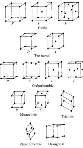
sions. There are 14 Bravais lattices, however, as summarized in Table 20-1. The possible point groups now include those with secondary axes and σ& planes, but are still restricted to Cx, C2, C3, C4 , and C6 principal axes. The various combina­

tions of symmetry elements consistent with each Bravais lattice give rise to 32 lattice types or lattice point groups. If combined rotation-translation and reflec­

tion-translation operations are included, then a total of 230 space groups are obtained. A three-dimensional crystal must belong to one of these space groups.

3

I \

F

j

Tetragonal 2

I

4/mmm

Orthorhombic 4 Ρ \

c ( F )

a φ b φ c

OC = β = γ = 90°

mmm

Monoclinic 2

c !

a Φ b φ c oc = γ = 90° φ β

21m Rhombohedral

(or trigonal)

1 Ρ a = b = c

oc = β = γ φ 90° ^3m

Hexagonal 1 Ρ a = b φ c

oc = β = 90°; y = 120°

6/mmm

Triclinic 1 Ρ a φ b φ c

α ^ j8 φ γ Φ 90°

m3m

°The symbols stand for: P, primitive, with lattice points only at the corners of the unit cell;

C, base centered; /, interior or body centered; F, centered on all faces, or face-centered.

b See Section 20-ST-l.

Clearly, the detailed treatment of all of these symmetry combinations is too long to be practical here, and we will confine ourselves almost entirely to some important examples in the cubic system.

We will, in fact, deal mainly with rather simple crystals—ones having atoms or ions at lattice corners or in lattice faces. Figure 20-3 shows the unit cell for a simple cubic lattice whose basis consists of an atom at each lattice point. A distinc­

tion to emphasize is that the unit cell is not necessarily the repeating unit. In Fig. 20-3 each corner atom is shared with eight adjacent unit cells and an attempt to generate the complete crystal by translations of this unit would superimpose atoms on each other. The repeating unit is in this case just the atom at the origin,

a

a

FIG. 20-3. Simple cubic lattice having one atom at each lattice point.

20-1 SPACE-FILLING LATTICES 853

X--

x—

- V

ι

Cubic

I ι ι

Ρ I Tetragonal

ι

ι

i

c /

Orthorhombic

Monoclinic Triclinic

I

Rhombohedral Hexagonal F I G . 2 0 - 4 . The 14 Bravais lattices.

that is, at position (0, 0, 0). If this atom is translated by all possible combinations of the unit lattice distance a, then the crystal is generated.

The number of atoms or ions in a unit cell is, of course, just the number present in the repeating unit. The same answer can be obtained from a diagram of the unit cell provided that corner atoms are counted as one-eighth of an atom each, face atoms as one-half, and so on. That is, each atom or ion is weighted according to the number of adjacent unit cells which share it.

Figure 20-4 shows the unit cells for the 14 Bravais lattices. These can be described by specifying the unit lengths a, b, and c and the angles oc, β, and γ as indicated in Fig. 20-5. The positions of the lattice points are then given in terms of this coordinate system. Thus the simple cubic unit cell has points (or atoms in the

F I G . 2 0 - 5 .

b

tetragonal, orthorhombic, hexagonal, and triclinic lattices, measured in units of (a, b, c) and along the required axis directions. The body-centered cubic lattice has the same positions as does the simple cubic lattice plus one at ( J , \, \); the face-centered cubic lattice has the additional points (|, 0), (0, J , J ) , 0 > i l )5 (h 1> έ ) > (h 0 ,1 ) , and Q , J , 1). In these last two cases the repeating units consist

of the points (0, 0, 0) and ( i J, \ \ and (0, 0, 0), ( i i 0), (0, i | ) , and (|, 0, | ) , respectively. Thus the body-centered cubic repeating unit has two points and the face-centered unit has four points. The same numbers would result if the unit cell points shown in Fig. 20-4 were counted as one-eighth if at a corner, one-half if on a face, and full weight if in the interior.

It is to be remembered that there will be actual crystals such that each point in Fig. 20-4 is occupied by a single atom, as just assumed, but many other crystals where each point is occupied by some molecule or grouping of atoms—a grouping whose symmetry is reduced from that of a sphere. Thus the lattice of crystalline carbon dioxide is face-centered cubic, but the basis consists of variously oriented C O2 molecules, as illustrated in Fig. 20-6.

20-2 Crystal Planes; Miller Indices

Any actual crystal is finite in extent and its surfaces are made up of planes that pass through lattice points. Thus ideal physical crystals are bounded by planes which are lattice or rational planes; the inverse reasoning was made by Hauy in 1784, namely that the regular shapes of crystals imply an inner regularity. How­

ever, the appearance of a crystal is very dependent on which planes bound it, as illustrated in Fig. 20-7 for a crystal whose lattice is cubic. As we truncate the corners of a simple cube progressively, surfaces corresponding to planes of the type indi­

cated in Fig. 20-8(a) increase in extent until the crystal is bounded only by such

20-2 C R Y S T A L P L A N E S ; M I L L E R I N D I C E S 855

planes. These different appearances are called crystal habits. It was gradually appreciated that it is not the crystal habit that is in itself fundamental, but rather its symmetry, especially the angles between crystal faces, and hence between crystal planes. One may often determine the point group to which a crystal belongs just from its external symmetry.

A system for characterizing rational planes was developed by W. H. Miller in 1839, using what are now called Miller indices. If we locate an origin at some lattice point, then any crystal plane must intercept the crystal axes originating from this point, as illustrated in Fig. 20-9. A theorem which we will not prove is that the three intercepts of any rational plane must be in the ratio of integers. This is known as the law of rational intercepts, due to Haiiy. Parallel to any such plane there is a whole set of planes which may be generated from it by application of unit translations along the axes of the lattice. If we now consider that plane of the set which is closest to the origin (without actually containing it), then the Miller indices (hkl) are the reciprocals of the intercepts, expressed in units of the lattice distances. In practice the indices (hkl) may refer either to this particular plane or to the whole set of equivalent ones.

\ v ι ^y

/ w / W / a

/ \ \ / a

^ > X

' χ I // I / ι / / I

1 1 / 1 /

κ /

/ ν

1 / / I s ' / f/'

(a) (b)

F I G . 2 0 - 8 . (a) The ( 1 1 1 ) plane of a cubic lattice, (b) The ( 1 1 1 ) plane of a cubic lattice.

To illustrate, the plane shown in Fig. 20-8(a) is the closest of its set to the origin and has the intercepts ( 1 , 1 , 1), expressed in units of a. The Miller indices are therefore the reciprocals, or (111). Other orientations are possible. Thus the plane shown in Fig. 20-8(b) has the intercepts (1, 1, —1), and corresponding indices (111). Similarly, the planes (111), (111), and so on exist. We will class all of these as just (111) planes in dealing with crystals in the cubic system.

Figure 20-10(a) shows a nearest-origin plane whose intercepts are (1, 1, oo) and corresponding Miller indices, (110). Planes parallel to one of the axes are more easily shown by means of a projection down that axis, as illustrated in Fig. 20-10(b), where the (110) planes now appear as set I. The intercepts for the nearest-origin plane of set II are (1, | , oo), giving the indices (120). Those for the planes of set III are left for the reader to determine. Note, incidentally, that the equation hx + ky + Iz = 1 is that of the plane nearest to the origin.

F I G . 2 0 - 1 0 . Various planes of a cubic lattice, (a) (110) plane, (b) Various (hkO) planes viewed down the ζ axis.

20-3 SOME SIMPLE CRYSTAL STRUCTURES 857

(b)

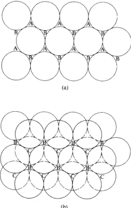
FIG. 20-11. Close packing of spheres, (a) First layer, (b) Second layer located with centers above krtype pockets of the first layer.

20-3 Some Simple Crystal Structures

A. Close Packing of Spheres

Many of the elements assume a crystal structure which corresponds to the closest possible packing of spheres. As illustrated in Fig. 20-11(a), a single layer of spheres forms a pattern having triangular pockets. There are two equivalent ways of locating the second layer, namely by placing the spheres either in the set of first layer pockets labeled A or in the set labeled B. If the A set is used, as in Fig. 20-11(b), then the Β set is excluded. The second layer again has two kinds of triangular pockets, those labeled B, which lie above the Β pockets of the first layer, and those labeled C, which lie above the centers of the first-layer spheres.

There are now two distinguishable ways of placing a third layer. If the spheres are put in the set of C-type pockets, they will lie directly above the first-layer spheres. The structure then repeats, the types of pockets in which successive layers rest being in the sequence ACACAC..., as shown in Fig. 20-12. The resulting symmetry is easier to visualize if the spheres are replaced by points at their centers, as in Fig. 20-13(a); the structure can now be seen to have hexagonal symmetry.

This arrangement is, accordingly, called hexagonal close packing, or hep.

Returning to Fig. 20-11(b), if the third-layer spheres are placed in the B-type pockets, this third layer will now have pockets of the A and C types. The next simplest repeating unit is then obtained by placing the fourth layer in the C pockets,

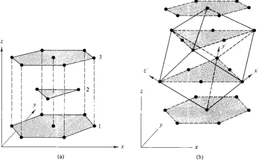
FIG. 20-12. Perspective view of (a) hexagonal and (b) cubic close packing of spheres.

(a) (b)

so as to be directly above the first layer (Fig. 20-12). The symmetry of the ABCABC arrangement is somewhat difficult to see. As shown in Fig. 20-13(b), we can trace the pattern of a face-centered cube by connecting points between the successive layers. Figure 20-14 shows the cube in a normal orientation; we now see more clearly that the successive layers of Figs. 20-12 and 20-13 correspond to (111) planes of a face-centered cubic lattice. The ABCABC arrangement is for this reason called cubic close packing, or ccp. Alternatively, of course, the structure is face-centered cubic, or fee.

It must be remembered that it is the symmetry and not the density of packing that differs between the hep and ccp structures. In both cases (but most easily seen in the hep symmetry), each sphere in a close-packed plane has six neighbors which are touching. There is a triangle of three nearest neighbors above and one below, to give 12 neighbors in all. In the hep structure the above and below triangles are

(a) (b)

FIG. 20-13. Perspective view of the positions of sphere centers in (a) hexagonal close packing, ACACAC sequence, and (b) cubic close packing, ABCABC sequences. Note in (b) the pattern that forms a face-centered cube with axes x', y', and z'.

20-3 SOME SIMPLE CRYSTAL STRUCTURES 859

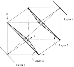
FIG. 20-14. Cubic close packing drawn so as to show the face-centered cubic lattice.

oriented in the same way, while in the ccp structure they are rotated 120° relative to each other. It may be shown, incidentally, that the close packing of spheres leaves 26 % void space.

Many metals crystallize in either the hep or the ccp structure, the choice appa­

rently being determined by relatively weak directional preferences in the metal- metal bonding. Metals having the hep structure include y-Ca, Cd, α-Co, j8-Cr, Mg, and Zn, while those having the ccp structure are Cu, Ag, Au, Al, Pb, j3-Ni, and y-Fe. The rare gases Ar, Ne, and Xe also crystallize in the ccp structure.

A definite tendency toward directed bonding appears with Zn and Cd; although the structure is approximately hep, the axial ratio c/a is 1.856 for Zn and 1.885 for Cd, as compared to 1.633 for closest packing. In other metals, this tendency leads to some other crystal structure, often body-centered cubic, or bcc. Metals showing bec structures include Ba, α-Cr, Cs, a-Fe, δ-Fe, K, Li, M o , N a , and j3-W. Notice that a given element may show more than one crystal modification, as in the case of Cr and Fe.

While hep and ccp structures both represent the closest packing of spheres, the physical proper­

ties of metals can be sharply dependent on which structure is present. Thus ccp metals tend to be much more ductile than hep ones. The reason is as follows. For crystals in general it is those planes that are the most closely packed which slip past each other most easily [note Eq. (20-5)].

There is only one such set of planes in the hep structure—namely the basal or hexagonal planes shown in Fig. 20-13(a). In the ccp structure, however, the close-packed planes are the (111) planes, and there are four of these, that is, there is a set of (111) planes, one normal to each of the four cube diagonals. In practice, one deals with metals which are polycrystalline, or have randomly oriented and mutually reinforcing crystal domains. As a consequence, the hep metals tend to resist distortion in any given direction since most of the crystallites will not be properly oriented for slip to occur. A much smaller fraction will be able to oppose slip in the case of a ccp metal.

β . Alkali Metal Halide and Other M X Structures

One of the early triumphs of x-ray diffraction was the determination of the crystal structure of sodium chloride. It consists of two interpenetrating fee lattices, as shown in Fig. 20-15, where, for clarity, the spherical ions are located by points

F I G . 2 0 - 1 5 . The NaCl structure of two inter­

penetrating face centered cubic lattices.

a

marking their centers. It must be remembered, however, that in any lattice whose positions are occupied by spheres, nearest neighbors are in contact (see Special Topics section). Thus Na+ and Cl~ ions are touching along the a axes, and the sum of the two ionic radii rN a+ + >ci- is a/2.

The NaCl type of structure is a fairly common one for MX-type salts. It is the structure of most of the other alkali halides (M = Na+, K+, and R b+, and X = F~, Cl~, Br~, and f ~, and CsF), as well as for compounds such as BaO, BaS, CaO, CaS, CdO, FeO, and other divalent metal oxides and sulfides. Ammonium ion acts like a spherical ion and N H4I also has the NaCl structure.

The figure gives the unit cell for NaCl; this is not, however, the repeating unit, which consists of four N a+ ions, at (0, 0, 0), (|, 0, | ) , (|, 0), and (0, | , | ) , and four CI- ions, at ( J , 0, 0), (0, £, 0), (0, 0, £), and (J, J , £). If this set is translated by all possible combinations of multiples of a in the x,y, and ζ directions, the entire crystal is generated. The same count of ions can be obtained from Fig. 20-15.

Na+ ions: (8 corner)! = 1 (6 face)i = 3 4 CI" ions: (12 edge)J = 3

(1 interior) 1 = 1 4

As a check in the counting of atoms, the proportion of each kind must always

F I G . 2 0 - 1 6 . The CsCl structure of two interpene­

trating simple cubic lattices.

20-3 SOME SIMPLE CRYSTAL STRUCTURES 861

BN ZnS (zincblende) ZnO FIG. 20-17. Typical MX lattices.

correspond to the stoichiometry of the formula of the compound. Notice also, as one characteristic of the NaCl structure, that each ion has six nearest neighbors, in an octahedral arrangement.

A second, and quite common, structure for M X salts is that of two inter­

penetrating simple cubic lattices, as illustrated in Fig. 20-16 for the best-known case, CsCl. The CsCl structure is also found for CsBr and Csl, as well as for other M X compounds, such as NH4C1 and N H4B r , and various intermetallic compounds, such as AgCd, AuZn, and CuZn. Each ion or atom has eight nearest neighbors, in square symmetry.

The NaCl and CsCl structures are only two of a number that M X compounds have been found to exhibit. Most such compounds, however, crystallize in one or the other of the structures shown in Fig. 20-17, each labeled according to its most prominent example. Notice that not all of the structures are cubic and that the number of nearest neighbors to a given kind of atom, or its coordination number, diminishes in the sequence:

lattice type CsCl NaCl ZnO ZnS BN coordination number 8 6 4 4 3 It should be apparent at this point that crystal structure does not correlate with the chemistry of a compound, nor with the atomic weights of the constituents per se. V. Goldschmidt, who determined many of the simple crystal structures around 1925, concluded that the structure of such crystals is determined by the stoichiometry of the compound, the ratio of atomic radii, and the polarizability of the units.

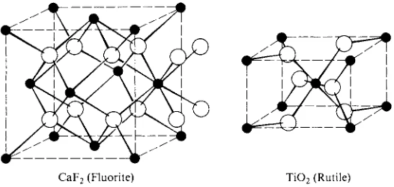
C. M X2 Structures

Two of the important structures for M X2 compounds are shown in Fig. 20-18.

For example, the form of T i 02 known as rutile crystallizes in the tetragonal system, with c = 4.58 Â and a = b = 2.98 Â. The unit cell contains two Ti atoms and four Ο atoms and is thus consistent with the formula of the compound. Each Ti has six Ο nearest neighbors and each Ο has three Ti nearest neighbors. If C denotes the coordination number in an MaX& compound, a useful rule of stoichi­

ometry is that

CMa = Cxb. (20-1)

CaF2 (Fluorite) T i 02 (Rutile) FIG. 20-18. Common M X2 structures.

D. Covaient Crystals. Diamond and Graphite

We next consider briefly two examples of covalent crystals, diamond and graph­

ite. In the case of diamond, the C—C bonds are of the covalent, sigma-bonded type, and show the tetrahedral bond angle of 109°28'. In a sense a diamond crystal is a single large molecule; the crystal structure, however, has a cubic unit cell, displayed in Fig. 20-19. As one way of visualizing the structure, notice that there is an atom at each corner, in the center of each face, and in the centers of alternate small cubes; one set of bonds is shown (the bond distance is 1.542 Â). Germanium, silicon, and gray tin have the same structure.

The diamond structure may also occur with covalent AB-type compounds, such as ZnS (zincblende) (see Fig. 20-17), Agi, CuBr, and BN. The atoms alternate in type, so each A and Β atom has four tetrahedrally disposed nearest neighbors.

Again, it is not the chemistry of the compound but primarily the relative size of the atoms and the geometry of their bonding that determine crystal structures in these cases.

Graphite serves as an example of a layer crystal. The structure is shown in Fig. 20-20 and is seen to consist of layers having a hexagonal tile pattern. The layers are aromatic in character; the C—C distance is 1.42 Â, or not much greater than the value of 1.397 Â for benzene. The distance between layers is relatively large, 3.40 Â, and the layer-layer bonds are consequently rather weak.

The high electrical conductivity of graphite can be regarded as due to the conjugation or aromaticity of the planes, which permits electrons to move through the crystal easily. The lubri­

cating property has been thought to stem from the ease of slippage of one layer over the next, but the actual situation has been found to be somewhat more complex. If graphite is thoroughly

FIG. 20-19. The diamond structure.

20-3 SOME SIMPLE CRYSTAL STRUCTURES 863

F I G . 2 0 - 2 0 . The graphite structure.

degassed, its coefficient of friction rises about sixfold, and it appears that gases adsorbed between layers are responsible for the very low friction ordinarily observed. The same may be true for a useful modern lubricant, M o S2, whose structure is analogous to that of graphite, as well as for other layer crystals, such as talc.

£. Molecular Crystals

The substances considered so far—metals, alkali metal halides and other ionic crystals, and covalent crystals—all have high melting points. This is a reflection of the strong bonds—metallic, ionic, or covalent—between the atoms of the lattice.

c

a

F I G . 2 0 - 2 1 . The benzene structure. [From E. G. Cox, D. W. J. Cruickshank, andJ. A. S. Smith, Proc. Roy. Soc. 2 4 7 , 1 (1958).]

FIG. 2 0 - 2 2 . Hexagonal (ordinary) ice. (Courtesy of Ν. H. Fletcher.)

A rather different situation exists in the case of crystals whose basis consists of stable molecules and which are therefore held together by secondary or van der Waals forces (note Table 8-8). Figure 20-21 shows the structure of crystalline benzene. This is a low-melting (6°C) white solid; it is soft and is not electrically conducting and clearly is made up of only weakly interacting benzene molecules.

The crystals of most simple molecules, such as 02, N2, CO, C 02, C H4, are of this type. Most nonionic organic substances also crystallize by virtue of van der Waals forces only, except where hydrogen bonding is involved.

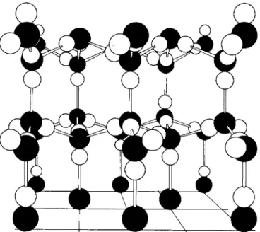
F. Hydrogen-Bonded Crystals. Ice

We conclude this section with a brief discussion of a remaining type of crystal structure, namely that in which hydrogen bonding is present. The most important example is undoubtedly that of ice, whose ordinary structure is shown in Fig. 20-22. It will be recalled from Fig. 8-8(b) that ice exhibits a number of crystal modifications, but only two, tetrahedral and hexagonal ice, are stable under atmo­

spheric pressure. It is the latter modification that is shown in Fig. 20-22. The basic structure is determined by the positions of the oxygen atoms; each is sur­

rounded tetrahedrally by four nearest neighbors at a distance of 2.67 Â. Only recently have advanced techniques using neutron diffraction (see Section 20-CN-l) established that the hydrogen atoms are located on the lines between oxygen atoms but asymmetrically placed; each oxygen is coordinated to two close hydrogen atoms and to two that are further away. The assignment of close versus far hydrogens is random, however, and in this respect the structure is disordered.

Hydrogen bonding is important in molecular crystals in which electronegative atoms, such as fluorine, oxygen, and nitrogen, can interact with an acidic proton of a neighboring molecule. This type of interaction becomes extremely important in crystals of biologically important substances, such as proteins and nucleic acids.

20-4 SOME GEOMETRIC CALCULATIONS 865

20-4 Some Geometric Calculations

The following types of calculations can be performed on any crystal but the geometric expressions rapidly become complicated as one departs from the cubic system. The general expression for the density of a crystal is, for example,

' = ^ ' (20-2)

where Πι is the number of the zth kind of atom (or molecule) of molecular weight Mi in the unit cell, and Vc is the cell volume. In the case of a cubic crystal Vc is just a3, while for a tetragonal unit cell Vc is a2c, and so on.

Two illustrations of the use of Eq. (20-2) follow. Iron (α-Fe) crystallizes in the bcc system with a = 2.861 Â; the eight corner and one interior atom in the unit cell give a net of two atoms, so

2(55.85) _= 7.92 g c m Q0 3 - 3.

6.02 χ 102 3(2.861 χ 10~8)3

Reference to Fig. 20-4 shows that each atom in a body-centered cubic lattice has eight nearest neighbors; the center atom, for example, must therefore be in contact with the eight corner ones and the body diagonal of the cube must equal two atomic diameters. The radius of each Fe atom is therefore

rFe - i V 3 (2.861 χ 10~8) == 1.24 Â.

Iron also crystallizes in the fee structure, and a reasonable assumption is that the radius of the atom does not change. In the cubic close-packed arrangement each atom has twelve nearest neighbors, and examination of either Fig. 20-4 or Fig. 20-14 shows that for a face-centered atom four of these neighbors consist of the atoms at the corners of the face. The face diagonal now contains two atomic diameters, or rFe = %V2a. On setting rFe = 1.24 Â, we obtain a = 3.50 Â for the fee structure. The unit cell has eight corner and six face atoms, or a net of four atoms, so the density of fee iron should be

4(55.85) Q „= 8.66 g c m 3 - 3.

r 6.02 χ 102 3(3.50 χ I O- 8)3

As a second illustration, the density of NaCl is 2.165 g e m- 3. There are four N a+ and four Cl~ ions per unit cell, so we have

4(22.99) + 4(35.45) 6.02 χ 102 3a3 '

whence # = 5.64Â. Reference to Fig. 20-15 shows that the closest distance between ions is that along a cube edge, so that a = 2 rN a+ + 2rC\- . The sum of the two ionic radii is then a/2 = 2.82 Â. As discussed in the Special Topics section, only sums of ionic radii may be determined from a crystal structure, but there are various schemes whereby individual ionic radii can be assigned.

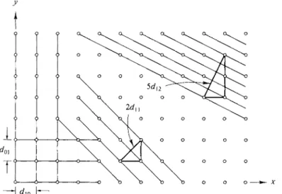
Another important type of calculation is that of the interplanar distances in a crystal. In the case of a two-dimensional, square lattice, illustrated in Fig. 20-23, it is obvious that (10) and (01) planes are spaced just a units apart, or that

^io = doi = a-> a nd likewise that dlx = \ \/2 a = 0.707a. The direction perpendi-

FIG. 20-23. Interplanar distances for a square lattice.

cular to (12) planes is evidently that of the diagonal of a rectangle of sides 1 and 2 in the χ and y directions, respectively. The particular diagonal shown is of length V5 a and spans five interplanar distances, sod12 = (1/V5 )a. The general formula is dhk = a/(h2 + k2)1!2. Extension to a three-dimensional cubic lattice gives

dhiti —

(h2 + k2 + I2)1'2 ' (20-3) or, for a lattice with a = β = γ = 90° but with α φ b φ c

1 d2

uhkl ~~ a2 + b 2+ c2 ^(20-4) Equation (20-3) gives the interplanar distance for planes of specified Miller indices, but it is sometimes convenient to class as belonging to a given type all planes which are parallel to each other, regardless of actual Miller index. Thus (100) and (200) planes may be called (100)-type planes, (111) and (222) planes may

FIG. 20-24. Interplanar distances in a bcc lattice.

20-5 DIFFRACTION BY CRYSTALS 867

be called (lll)-type planes, and so on. The distinction is illustrated further as follows. The largest interplanar distances for a simple cubic crystal are, in order,

^100 ? ^ n o » a nd ^ i i i ? a nd their ratios are given by Eq. (20-3) as simple cubic: d100 : d110 : dul = 1 : : .

v2 v3

The largest interplanar distances for a bcc lattice are, again in order, d110, d200 , and d222 (s ee Fig- 20-24):

110 200 222 ^ 2 2 2 ^{V 3}

These latter two planes may be referred to as (100)- and (11 \)-type planes, however, and the ratios reported as

bcc (type planes): d100 : d110 : dul = ^ : ~ : —^— = 1 : • 2 1 Similarly,

2

V2

Λ/2 v3

(the demonstration is left to the reader). As will be seen in the next section, x-ray diffraction studies may in some cases yield an interplanar spacing where the type but not the actual Miller index of the planes is known.

A final point of geometry is the following. In the case of simple structures it will often be true that a set of planes contains all of the atoms or ions of the crystal. Thus if a metal crystallizes in the bcc structure, the (200) planes as a set pass through or contain all of the atoms of the crystal. The same is true for the sets of (110) and (222) planes. The crystal can thus be viewed as consisting of layers of (200) planes having a surface concentration σ2 00 atoms c m-2 and separated by d200 cm. The quotient σ2 0 0/ί/2 00 must therefore equal the volume concentration of atoms in the crystal, C atoms c m- 3. The crystal can alternatively be regarded as consisting of layers of (110) planes separated by d110, so that a110/d110 = C. Thus for any set of planes which contains all the atoms of the crystal, it follows that

^ = C. (20-5) dhkl

Equation (20-5) is often quite useful. It tells us that the highest surface density of atoms will occur on that set of planes of largest interplanar spacing. These are the (110) planes in the bcc structure and the (111) planes in the fee case, for example. Such planes tend to have the lowest surface free energy and therefore tend to be prominent faces in actual crystals. They also tend to slip or to cleave the most easily, as is noted in Section 20-3A.

20-5 Diffraction by Crystals

X rays were first observed in experiments around 1890 with cathode ray tubes (see Section 22-1); by 1895 J. J. Thomson was describing the effect of this pene­

trating radiation on the electrical properties of gases. Later, in 1898, G. G. Stokes and G. J. Stoney suggested that χ rays were electromagnetic in nature and the classic first experiment establishing x-ray diffraction was done in Munich in 1912 at the suggestion of M. von Laue.

2 2 2

radiation of this energy per quantum is

corresponding to 1.44 Â. X-ray wavelengths are thus comparable to atomic radii.

Modern equipment still consists essentially of a Crookes tube, in which a beam of perhaps 20-kV electrons impinges on a target, usually copper, iron, or tungsten.

The emitted χ radiation is generally filtered (see Section 22-4 on the critical absorp­

tion of χ rays) and then collimated by means of slits so as to produce a narrow, monochromatic beam.

Before discussing three-dimensional diffraction effects it should be explained why it is that χ rays act as though they are reflected specularly from each plane of a crystal. The interaction of an x-ray quantum with an atom may be regarded as an absorption followed by resonance emission (Section 19-3), that is, by emission at the same wavelength. This process is a virtual one; it constitutes a hypothetical mechanism yielding the same result as does the wave mechanical treatment of scattering. The eifect is that each atom becomes a secondary, isotropic emitter of the χ radiation, as illustrated in Fig. 20-25 for a single line of atoms.

A more detailed analysis is as follows. We suppose there to be incident radiation at angle θ to the line of atoms ABC. The radiation first hits atom A, which then emits isotropically, and by the time the wavefront reaches atom Β the secondary radiation from atom A has a wavefront given by circle I A. When the radiation reaches atom C the wavefronts of secondary radiation for atoms A and Β are now given by circles 2A and IB. Still later the reemitted radiation has reached circles 3A, 3B, and 3C. Where similarly numbered circles cross, the emitted radiation is in phase, as for example, at point a, the crossing between circles 2A and 2B, and

(8584)(8.066) = 6.92 χ 104 kK - 6.92 χ 107 c m -1,

FIG. 20-25. Scattering of χ rays from a single line of atoms.

20-5 DIFFRACTION BY CRYSTALS 869 point b, the crossing between circles 3A and 3B. As the circles move outward with time, the line along which the radiation is in phase is that given by the line ab.

Alternatively, points b and c represent concurrent in-phase conditions and define the wavefront of the secondary radiation. Either reasoning leads to the conclusion that the direction of the secondary radiation is at the same angle θ to ABC as is the incident radiation, independent of the spacing between atoms, provided it is uniform.

This analysis is geometric and qualitative but serves to explain the rigorous result that the secondary radiation is mutually interfering except in the direction of specular reflection. We may now proceed to the three-dimensional situation.

A. The Bragg Equation

The first diffraction experiment was made with the use of "white" χ radiation, that is, radiation having a range of wavelengths, and a single crystal (of copper sulfate). Later, around 1912, W. Bragg and his son developed an approach which was, at that time, much easier to apply and to interpret. This consisted in using monochromatic χ radiation and varying the orientation of the crystal.

The situation is illustrated in Fig. 20-26. We take each ray of incident radiation to be specularly "reflected" by a given layer of atoms, shown end-on in the figure.

Reflections then occur from the successive layers, and we now ask what condition must be met for the reflected radiation to be in phase. Considering just the first two layers, the difference in path length for the respective rays is the distance abc.

From the construction, this distance is lab or 2d sin Θ. Thus 2d sin θ must be an integral number of wavelengths if the reflected radiation is to be in phase. The Bragg condition is thus

ηλ = 2d sin 0, (20-6) where η is an integer. If η = 1, the reflection is called first order, if η = 2, second

order, and so on. Note, however, that a second-order reflection for a given spacing d is at the same angle as a first-order reflection from planes of spacing d/2. Thus second-order reflections from (100) planes of a simple cubic crystal should be indistinguishable from first-order reflections from a hypothetical set of (200) planes.

It is more convenient to treat the order of a reflection in this alternative way and

FIG. 20-26. The Bragg scattering condition.

sin2 θ = (h2 + k2 + I2). (20-8)

β . Bragg Diffraction Patterns

Figure 20-27 shows schematic plots of reflected intensity / versus θ for KCI and NaCl. A single crystal is oriented so that (100)-, (110)-, or (lll)-type planes (or crystal faces) are perpendicular to the x-ray beam and the crystal is then rotated so that the angle of incidence θ is varied. As the angles for successive Bragg condi­

tions are met, an increase in intensity of scattered radiation is observed by means of a detector whose angular position is also rotated so that it always "sees"

radiation at the specular angle. The schematic arrangement is shown in Fig. 20-28.

In the case of NaCl the first-order peaks are found in a particular experiment to occur at 5°18', 7°31', and 4°36' for reflections from (100)-, (110)-, and (lll)-type planes, respectively. The interplanar distances are then in the ratio of the recip­

rocals of the sin θ values, or d100 : d110 : dlu = 1/0.0924 : 1/0.1307 : 1/0.0801 = 1:0.707 : 1.154 = 1:1/ Λ/2 : 2 / V 3 . This is just the ratio predicted in the preceding section for a fee structure. The early experimentalists knew from the symmetry of

F I G . 2 0 - 2 7 . Intensity versus θ for Bragg scattering from (100)-, (110)-, and (11 \)-type planes of (a) NaCl and (b) KCI.

20-5 DIFFRACTION BY CRYSTALS 871

FIG. 20-28. A Bragg x-ray spectrometer.

NaCl crystals that they were in the cubic system and from the ratio test could determine which type. By reversing the density calculation of the preceding section, a could be calculated, and from this the wavelength of the χ rays used.

Most other alkali halide crystals show an analogous set of intensity patterns but, as illustrated in Fig. 20-27(b), that for KCl gives sin θ values of 0.0811, 0.1145, and 0.1405 for reflections from (100)-, (110)-, and (lll)-type planes, respectively, using the same χ rays. This yields a set of ratios d100 : d110 : dni = 1: 0.707 : 0.577 = 1 : 1 /Λ/ 2 : 1 /Λ/ 3 , or that corresponding to a simple cubic structure.

Referring to Fig. 20-15, the explanation lies in the nature of the ( l l l ) - t y p e planes.

In the case of NaCl the N a+ ions are contained by one set of (111) actual planes and the C l_ ions, by a second set lying midway between. The reflections from the (111) actual planes are partially but not completely canceled by the out-of-phase reflections from the planes containing the other kind of ion. Thus in Fig. 20-27 the first peak for (lll)-type planes for NaCl is weaker than usual. In the case of KCl the two ions are isoelectronic and scatter χ rays about equally; the effect is that K+ and Cl~ ions appear to be identical in the diffraction experiment. Reflec­

tions from the Cl~ (lll)-type planes therefore cancel those from the K+ (111)- type planes. The result is that the largest interplanar distance showing a net diffraction intensity is that for (222) actual planes. Alternatively expressed, χ rays do not distinguish K+ from Cl~ and KCl appears as a simple cubic lattice of side a/2, where a is the side of the actual fee unit cell.

The example is introduced to illustrate the point that the intensity of Bragg reflections from a given (hkl) set of planes depends on the densities and nature of atoms on these and on intervening planes as well. A more formal approach is given in Section 20-ST-2.

C. Powder Patterns

The Bragg method is not only historic but is also of current usefulness. The application is mainly to a crystalline powder. The individual particles are assumed to be in random orientation, so that the monochromatic χ rays will always find some particle with the correct orientation for reflection from each (hkl) set of planes. The experiment consists in irradiating a thin tube filled with the powdered sample, using a collimated beam of monochromatic χ rays. Those crystals whose

Tube c o n t a i n i n g p o w d e r sample

x-ray beam

particular (hkl) planes are at the Bragg angle θ to the beam then give a reflection at an angle Θ to the crystal planes, or 2Θ to the incident beam. As illustrated in Fig. 20-29, one may use a circular strip of photographic film to intercept the diffracted radiation, which then shows as curved lines on the film. Alternatively, a traveling radiation counter may be used. The sin θ value for each line is calculated from the apparatus geometry.

The next task is to assign (hkl) values to the lines. This can be done if the crystal is known to be in the cubic, tetragonal, or orthorhombic class but is otherwise rather difficult. Often the "powder pattern" is used much as are infrared absorption spectra, namely as a kind of fingerprinting of the particular substance. A mixture of materials may then be analyzed semiquantitatively by calculating in what proportion pure substance powder patterns are present.

The procedure for assigning actual (hkl) values to individual lines can be illu-

TABLE 20-2. Indices of Cubic Crystals a Allowed reflection

Indices Simple

(hkl) h2 + k2 + /2 cubic bcc fee

100 1 X

_

110 2 X X

111 3 X

—

200 4 X X X

210 5 X

—

211 6 X X

220 8 X X X

300, 221 9 X

— —

310 10 X X

311 11 X

—

222 12 X X X

320 13 X

— —

321 14 X X

—

400 16 X X X

aT h e sum of the squares of three integers cannot have the values (7 + 8m)4n, where m and η are arbitrary integers.

COMMENTARY AND NOTES, SECTION 1 873 TABLE 20-3. Sample Treatment of Powder Diffraction

Data for Lead

Result of Integers Observed dividing by having these

sin2⁰ 0.073 ratios (hkl)

0.0729 1 3 (HI)

0.0977 1.33 4 (200)

0.194 2.65 8 (220)

0.267 3.65 11 (311)

0.291 4.01 12 (222)

0.389 5.33 16 (400)

strated fairly easily if the crystal is in the cubic system. From Eq. (20-8) the sin2 θ values are proportional to h2 + k2 + I2. The first step is to tabulate the film data in order of increasing sin2 Θ. Since h2 + k2 + I2 must be an integer, we then look for the smallest set of integers that are in the ratios of the sin2 θ values. Only certain integral values for h2 + k2 + I2 are possible for each type of cubic crystal.

In the case of a simple cubic crystal, the sum cannot have the values 7, 15, or 23, for example, since there are no three integers the sum of the squares of which equals one of these numbers. The sum can only have the values 2, 4, 6, 8,... for a bcc crystal and only the values 3, 4, 8, 11, 12,... for a fee one, as summarized in Table 20-2. We can then determine which set the observed series of sin2 θ values matches.

An example should be helpful at this point. We suppose that a particular sample of finely divided lead shows the following sin2 θ values with χ rays of 1.54 Â : 0.0729, 0.0972, 0.194, 0.267, 0.292, and 0.389. The procedure is shown in Table 20-3. We first divide each number by 0.0729 and observe that the result is not a set of integers. Examination indicates that multiplying each number by three will yield integers, as shown in the third column. These integers are just those allowed by Table 20-2 for a fee structure, and we then index each entry accordingly.

In an actual experiment each sin2 θ value would now be divided by the assigned h2 + k2 + I2 value to obtain a series of values of λ2/4α2, which would be averaged.

In the present example we take this average to be 0.0729/3 = 0.0243, and from the known λ of 1.54 Â calculate a to be 4.94 Â. We could proceed to check the result by calculating the density of lead.

COMMENTARY AND NOTES

20-CN-l Modern Crystal Structure Determination

The presentation in Section 20-5 emphasized the Bragg method and powder patterns as a straightforward yet actively useful approach to x-ray diffraction. It is not, however, the method used for crystal structure determination where any degree of complexity exists. The difficulty with the Bragg method is that of indexing

orientation of the crystals that give a particular reflection. These methods are described briefly below.

Once a set of reflections has been indexed and their intensities measured, the next problem is that of deducing the crystal structure. The lattice type or symmetry can often be determined from an examination of a crystal under a polarizing microscope. The symmetry of the crystal habit helps to establish the Bravais lattice involved; the behavior under polarizing light may suffice to limit the space group to at least a few possibilities. The presence or absence of certain reflections is usually sufficient to complete the assignment.

A. Rotation-Oscillation Methods

One gains enormously in ability to index diffractions by using monochromatic χ radiation and a single crystal which can be mounted so that one of its crystal axes is perpendicular to the x-ray beam. In the rotating crystal method, as the crystal turns various planes come into the Bragg angle with respect to the incident beam. The diffraction consists of spots generated in a series of horizontal layers on the film, as illustrated in Fig. 20-30. Those reflections at the same level as the crystal arise from planes parallel to the rotation axis, and those reflections above and below arise from planes whose inclination to the axis can be calculated. Thus each spot can immediately be assigned one index. The remaining indexing can still be very difficult if the crystal has many atoms in the unit cell, and a yet better procedure is available.

The next step is to displace the film synchronously with what is usually an oscillation rather than a continuous rotation of the crystal. In this way the orien­

tation of the crystal is known for each diffraction spot. The Weissenberg method, as it is called, thus allows each spot to be fully indexed. The method produces series of diffraction spots which lie on curved lines, however, and in the precession

Crystal rotated about c axis

x-ray beam hkl

hkl

F I G . 20-30. Rotating crystal method.

COMMENTARY AND NOTES, SECTION 1 875

method, the motions of the crystal and the film are so regulated that the spots lie on straight lines.

β . Electron Density Projections

A crystal appears to χ rays as a collection of scattering centers, each of intensity approximately proportional to the number of electrons possessed by a particular atom in the unit cell. The information provided by x-ray diffraction is therefore that of the distribution of electron density p(x, y9 z) in the crystal. Since this distribution is a periodic one, it is very convenient to represent it as a set of cosine and sine terms—that is, as a Fourier series.

The formal expansion of p(x, y, z) is

where V is the volume of the unit cell and Fhkt is called the structure factor (see Section 20-ST-3). This form recognizes that the electron density is periodic with repeat distances of a, b, and c. If one could evaluate each term from the diffraction data, the resulting p(x, y, z) would be the crystal structure. The problem is that the intensity measurements yield | Fhu |2 but not the sign of Fhkl itself.

A number of rather sophisticated procedures have been developed to help get around the problem. It is possible, for example, to determine the distribution of interatomic distances from the indexed intensity data alone. With this information and some educated guesses the crystallographer may be able to arrive at a trial structure. Even if approximate, such a structure will allow a calculation of the sign of each FhkU and now the experimental intensity data can be used to calculate an actual p(x, y, z). The result usually appears as electron density contour maps calculated for one or another projection. Such a result for anthracene is shown in Fig. 20-31.

Another "trick" is to incorporate very heavy atoms (such as iodine) in the molecule. The intense scattering by such atoms dominates the diffraction pattern and it may be possible to determine the positions of the heavy atoms and thus the sign of their F factor. Sometimes a natural grouping, such as a benzene ring, can be recognized in the diffraction pattern and subtracted from it.

C. Use of Radiation Other than X Rays

The fundamental equations of this chapter are not restricted to any particular kind of radiation. The main restriction is that inherent in the Bragg equation, namely that since sin θ cannot exceed unity, λ must be less than dm\2. Thus the wavelength of the radiation used must be less than half of the interplanar spacings to be determined. This means that radiation of no more than about 1 Â can be used.

In view of the de Broglie relationship (16-7), particles have a wave nature and should also exhibit diffraction effects. Thus 40,000-eV electrons would have (4 χ 104)(1.602 χ I O- 1 2) = 6.408 χ 10~8 erg kinetic energy, corresponding to a

(20-9)

momentum of 1.075 χ 1 0 "17 g cm s e c- 1. The wavelength is then 6.625 χ 10"2 7/1.075 χ I O "17 = 0.0616 Â. Electrons of this energy do indeed show diffraction effects and may be used for structure determinations. Electrons, being charged, interact more strongly with matter and are more rapidly absorbed than is χ radiation. As a consequence, very thin samples must be used. Standard electron microscopes may, for example, be put in a diffraction mode of operation so as to show the diffraction pattern for very thinly sliced samples. Because electrons can be focused by means of magnetic lenses, it is also possible to obtain a direct picture.

Figure 20-32 shows a modern high-resolution electron microscope photograph of a thin flake of N b2 20 54 . In this photograph, the view is down the b axis of the crystal; the white areas are channels between columns of N b 06 octahedra, and the dark circles correspond to columns of tetrahedrally coordinated Nb atoms.

Returning to diffraction studies, we find that it is possible to obtain molecular structures from the diffraction of a monoenergetic beam of electrons by a molecular gas. The situation here is similar to that of the powder method since each individual molecule is in random orientation, and the analysis is similar except that one now deals with distances between atoms in a molecule rather than with interplanar

COMMENTARY AND NOTES, SECTION 2 877

distances. One finds for the intensity of the scattered beam at angle θ

s i n χ*

where F is the atomic scattering factor, and xtj is given by

4 7 7 Tiy . θ

IL cm

Xij — s i n :

(20-10)

(20-11) The distances r{j are those between atoms / and j in the molecule. Equation (20-10) is known as the Wierl equation. It is possible to transform the Ι(θ) results into a radial distribution function (much as in the case of Fig. 8-1) and from this one can usually infer the molecular bond lengths and angles.

Alternatively, neutron scattering may be employed. The same calculation as the preceding applies but now with m equal to the neutron mass, about 2000 times larger than that of the electron. Neutrons of momentum 1.08 χ 1 0- 17 g cm s e c- 1, and hence wavelength 0.0616 Â, have 1/2000 the energy or about 3 χ 1 0- 11 erg m o l e c u l e- 1, corresponding to a "temperature" of about 1000 K. Neutrons of thermal or room-temperature energy have wavelengths, then, of around 1 Â and such neutrons may be provided by nuclear reactors (see Section 22-CN-2). A velocity selector (such as illustrated in Section 2-CN-2) may then be used to provide a monoenergetic beam. The technique is a relatively difficult one, and the chief advantage in using it is that, unlike the case with χ rays, the scattering of neutrons is large for light atoms. Neutron diffraction has, for example, been used to locate protons in ice and in metal hydrides, a very difficult task with χ rays.

FIG. 20-32. High-resolution electron micrograph of the N b

2

54

which modern crystallography has been developed. A number of high-molecular- weight biological materials can be obtained in crystalline form, and some extremely difficult structure analyses have been made on such crystals.

One of the great triumphs of x-ray crystallography is the determination of the structure of vitamin B12 by Dorothy Hodgkin and her co-workers. The formula of this very complex molecule is shown in Fig. 20-33 ; it consists of two principal parts, a nucleotide and a coordination complex of Co(III). The cobalt ion is chelated to four nitrogen atoms in a square planar ring and to cyanide ion and another nitrogen atom along the axis perpendicular to the ring. The entire structure, except for the cyanide, is called cobalamin. The analysis of the many thousands of individual diffraction spots to finally obtain the three-dimensional structure of vitamin B12 required the joint effort of a large international team of investigators.

A second crystallographic triumph was the determination of the structure of hemoglobin, illustrated in Fig. 20-34. This is, of course, a large protein molecule, a principal function of which is to coordinate an iron atom (shown in the figure).

The iron reversibly takes up a molecule of oxygen, thus giving hemoglobin its oxygen-carrying property. More recently, a great deal of crystallographic work has been done on the structure of nucleic acids, R N A (ribonucleic acid) and D N A (deoxyribonucleic acid). We are now dealing with molecular weights up to several million, and while x-ray diffraction has confirmed the double helical structure, complete structural analyses have not so far been possible (see Section 21-6).

FIG. 20-33. Structure of vitamin B1 2. The cyanide attached to the Co atom is introduced during the isolation and crystallization procedure.

COMMENTARY AND NOTES, SECTION 3 879

FIG. 20-34. Structure of hemoglobin. (Courtesy of J. C. Kendrew.)

20-CN-3 The Band Model for Solids. Semiconductors

We have so far considered a crystal to be made up of discrete atoms in a repeat­

ing structure. The wave mechanical picture, while basically not much different, does introduce an aspect of great importance with respect to the energy levels of electrons in a crystal. The point is that while completely isolated atoms would have energy levels as described in Chapter 16, when these are brought into proximity in a crystal, electron exchange begins to be possible. Suppose, for example, we had a crystal consisting of hydrogen atoms, or, more realistically, of hydrogen- iike atoms, such as lithium. Considering first just one pair of atoms, then, as given by Eqs. (18-13) and (18-14), the single equal energy states of each atom combine to give a bonding and antibonding pair. In terms of the present dis­

cussion the point is that the mixing of wave functions between two atoms generates a pair of new states, one above and one below the original isolated atom state.

In a crystal some number Ν of atoms mix their electrons wave mechanically,

2s

ls

Lattice spacing

FIG. 20-35. Splitting of energy levels as two atoms approach.

and the result is Ν states distributed in a band roughly centered at the original isolated atom state. The degree of this mixing increases as the atoms approach, and the situation is shown schematically in Fig. 20-35. In the case of a crystal of lithium the band due to the ls states does not span enough range of energy to overlap with that from the 2s ones. The ls band will have Ν states and just IN electrons, that is, two ls electrons from each atom, to exactly fill it.

The 2s band is only half-filled, however, since only TV outer electrons are present.

There are thus many close-lying excited states accessible to these electrons, with the consequence that they have a Boltzmann-type distribution of kinetic energies and can move easily from one point to another. Hence the electrical conductivity of lithium.

A metal such as beryllium would exactly fill its 2s band, but it turns out that the 2p overlaps with it, so that again the outer electrons are able to move freely. The wave mechanical picture of metallic conduction is thus one of bands only partially filled with electrons. The mobility of the electrons is adversely affected by the thermal vibrations of the lattice, which disrupt its regularity. As a consequence, metallic conductivity tends to decrease with increasing temperature.

The profile of a band, that is, the plot of N(E), the number of energy states, versus energy E, might look as in Fig. 20-36. Metals correspond to the situation shown in Fig. 20-36(a,b), that is, to an incompletely filled band or to overlapping bands. If, however, the highest energy band is completely filled and well separated from the next one, then electrons cannot move since there are no easily accessible excited states; the substance is then an insulator. An example is diamond, which has a completely filled band well separated from the next higher one, as in Fig. 20-36(c). Finally, it may happen that while a band is filled, the next higher one is so close that little additional energy is needed to promote electrons to it, as illustrated in Fig. 20-36(d). Such a substance will show an electrical conduc­

tivity which strongly increases with temperature, as the electron population of the

COMMENTARY AND NOTES, SECTION 4 881

upper band increases and leaves vacancies in the lower one. Such materials are called intrinsic semiconductors. Germanium has an energy gap of 0.72 eV, and gray tin one of only 0.1 eV; both behave in this manner.

It is also possible to produce electron mobility by incorporating suitable impur­

ities in the lattice of an insulator or intrinsic semiconductor. The impurity should be able to substitute for one of the regular lattice atoms so as not to distort the lattice appreciably. Suppose, for example, a boron atom is substituted for carbon in the diamond lattice or for silicon or germanium in their crystals. The boron atoms act as C+, S i+, or G e+ ions, being one electron short, and the effect is to produce holes or vacancies in the highest energy band. The energy match is not exact, and while the boron atoms act as acceptors of electrons, some promotion energy is needed. Similarly, if Ρ atoms are introduced, these act like C~, S i-, or Ge~ atoms, and with a little additional energy the extra electron can be promoted into the next higher unfilled band of the crystal. The effect of either impurity is to greatly increase the semiconductor property of the crystal. Such crystals also tend to exhibit photoconductivity since light energy can also promote electrons to allow conduction.

It might be mentioned that the bands in an insulator (which do not overlap) are not uniform through the crystal but are bounded geometrically by zones called Brillouin zones the shapes of which are determined by the crystal symmetry.

The situation can be viewed as a confinement of electrons due to their reflection by crystal planes. In conductors, the Brillouin zones overlap, so that free motion through the crystal is possible.

20-CN-4 Crystal Defects

Actual crystals do not consist of the perfect lattice array implicit in the discus­

sion so far. First, many apparently crystalline materials are actually microcrystal-