1Hungarian Academy of Sciences, Hungarian Danube Research Institute, Jávorka Sándor út14, H-2131 G¨od, Hungary
2E¨otv¨os Loránd University, Department of Systematic Zoology and Ecology, Pázmány Péter sétány 1/c, H-1117 Budapest, Hungary
3AL ¨OKI Applied Ecological Research and Forensic Institute Ltd., Kassa utca118, H-1185 Budapest, Hungary
4“Adaptation to Climate Change” Research Group of the Hungarian Academy of Sciences, Villányi út 29–43, H-1118 Budapest, Hungary; e-mail: leventehufnagel@gmail.com
Abstract:Ecological models have often been used in order to answer questions that are in the limelight of recent researches such as the possible effects of climate change. The methodology of tactical models is a very useful tool comparison to those complex models requiring relatively large set of input parameters. In this study, a theoretical strategic model (TEGM ) was adapted to the field data on the basis of a 24-year long monitoring database of phytoplankton in the Danube River at the station of G¨od, Hungary (at 1669 river kilometer – hereafter referred to as “rkm”). The Danubian Phytoplankton Growth Model (DPGM) is able to describe the seasonal dynamics of phytoplankton biomass (mg L−1) based on daily temperature, but takes the availability of light into consideration as well. In order to improve fitting, the 24-year long database was split in two parts in accordance with environmental sustainability. The period of 1979–1990 has a higher level of nutrient excess compared with that of the 1991–2002. The authors assume that, in the above-mentioned periods, phytoplankton responded to temperature in two different ways, thus two submodels were developed, DPGM-sA and DPGM- sB. Observed and simulated data correlated quite well. Findings suggest that linear temperature rise brings drastic change to phytoplankton only in case of high nutrient load and it is mostly realized through the increase of yearly total biomass.
Key words:climate change; ecological model; nutrient load; tactical modeling
Introduction
Beyond doubt, in order to recognize the effects of global changes expected in the future the methodology of eco- logical modeling seems to be a very useful tool. Ques- tions related to the hazards of global warming are in the focus of attention in recent science literature (Ladányi
& Horváth 2010). Ecological modeling with different temperature data series (e. g. data series of climate change scenarios) provide an excellent opportunity to forecast possible future states attributable to the global warming in aquatic environments as well. On the one hand, it can be used for hypothesis testing concern- ing the effects of physical changes (e.g. change in water temperatures or inflow) in different aquatic habitats on the biota. On the other hand, one can make quantita- tive predictions about the effects of climate change by the application of climate models.
A number of modeling approaches have been pro- posed in order to sketch the main trends in variation of physical, chemical and biological components of fresh- water systems under the pressure of climate change.
Some models aim to describe the variation of environ- mental parameters of certain lakes or rivers, so one can extrapolate those findings to the biota or community only on the basis of recent knowledge (e.g. Hostetler &
Small 1999; Blenckner et al. 2002; Gooseff et al. 2005;
Andersen et al. 2006). Other models are devoted to answer related questions of certain water bodies (e.g.
Matulla et al. 2007; Hartman et al. 2006; Peeters et al.
2007), which can be of great use, but also their method- ology can be adapted to other questions or habitats.
Complex ecosystem models (e.g. Elliott et al. 2005;
Mooij et al. 2007; Komatsu et al. 2006; Malmaeus &
H˚akanson 2004; Krivtsov et al. 2001), incorporating most fundamental processes of freshwater systems, are the keys to understand the effects of climate change from a broader aspect. Modeling methodology, which brings relevant pieces of information to the field of cli- mate change research, is however rather fuzzy now (Sip- kay et al. 2009b). This shortcoming is due to their com- plicated applicability and the lack of complex models.
These models require quite a lot of information as in- put parameter, which are often not available. Often one
* Corresponding author
c2012 Institute of Botany, Slovak Academy of Sciences
manages to set up a complex model, but its parameters cannot be determined due to lack of field data. Thus, instead of complex ecosystem models often are used tac- tical ones, which focus on the essence and may neglect some important pieces of information at the same time.
(In general, the “tactical model” is a model prepared in order to make predictions, to provide solution for prac- tical problems.) Still they can be a useful tool in under- standing the general functioning of the system. This is achieved through stressing the importance of the fac- tor regarded as the most crucial one and neglecting the other processes (Hufnagel & Gaál 2005; Sipkay et al.
2008a, 2008b; Sipkay et al. 2009a; Vadadi-F¨ul¨op et al.
2008, 2009).
The aim of the present study was to simulate the seasonal dynamics of phytoplankton by means of a dis- crete, deterministic model based on the data collected in the Danube River at the station of G¨od (1669 rkm), Hungary. A “strategic model”, which is considered as a theoretical simulation model, the so-called TEGM (Theoretical Ecosystem Growth Model, Drégelyi-Kiss et al. 2008, Drégelyi-Kiss & Hufnagel 2009a, Sipkay et al. 2010, Hufnagel et al 2010) was used as a starting point. Within this tactical approach, predictability was considered as primary purpose by stressing few factors expected as crucial driving forces instead of creating a rather complex ecosystem model considering all en- vironmental and biotic factors accounting for phyto- plankton production (Sipkay et al. 2009b; Hufnagel &
Gaál 2005). Treating temperature as the most signif- icant factor in seasonal dynamics modeling seems to be obvious. The model assumes that temperature is the only factor accounting for biomass variation, thus, the pattern is determined by the daily temperatures, other environmental factors – e.g. trophic links, inter- population interactions – appear within this term or are hidden. In addition, reaction curve describing tem- perature dependence is expected to be the sum of opti- mum curves because the individual optimum curves of species and groups add up to the optimum curves of the community. The availability of light needs to be taken into consideration as well according to recent knowl- edge on phytoplankton of the Danube River (Kiss 1994, 1996).
Moreover, the authors consider that decreased an- gle of incidence limits winter phytoplankton grow.
We also needed to consider the length of the avail- able field data. We can take full advantage of long-term (i.e.>6 years) surveys in virtually every field of inter- est (Kaur 2007), but they become increasingly valuable from the point of view of climate change. The inten- sive sampling frequency makes the data of the Hungar- ian Danube Research Station able to being employed in simulation models dependent upon weather conditions.
The aim of this study was to develop a tactical model, which can answer questions of potamoplankton seasonal dynamics by means of temperature data as input parameters. Within this framework, the authors propose a model of extensive applicability for global warming related issues. Within a simplified model situ-
ation, the possible effects of warming on phytoplankton biomass of the Danube River were analyzed.
Material and methods
Phytoplankton was sampled weekly from the Danube River at the station of G¨od (1,669 rkm) throughout the period of 1979–2002, within the continuous plankton recorder pro- gram of the Hungarian Danube Research Station of the Hun- garian Academy of Sciences (Kiss 1994). Samples were taken from the surface water layer and preserved with Lugol solu- tion. Phytoplankton was measured quantitatively according to the Uterm¨ohl method (Uterm¨ohl 1958).
Phytoplankton data were presented as biomass in mg L−1. Biomass was calculated by considering density and biovolume of specimens. When calculating biomass, correc- tions factors were added describing the dependence on sea- son and hydrologic regime. The investigation was long-term (longer than 6 years), which makes the data good for mod- eling.
First, the so-called “TEGM” – Theoretical Ecosystem Growth Model (Drégelyi-Kiss & Hufnagel 2009a, 2009b) – was used, which is the model of a purely theoretical algal community covering the potential temperature spectrum by the help of temperature optimum curves of 33 theoretical species. These theoretical species include 2 supergeneralists, 5 generalists, 9 transients and 17 specialists according to their degree of tolerance.
The strategic model of the theoretical algal commu- nity was adapted to the measured data resulted in the tac- tical model of DPGM (“Danubian Phytoplankton Growth Model”). Model fitting was performed using the Solver op- timizer program of MS Excel.
During model fitting it was also taken into account that throughout the 24-year long sampling period (1979–
2002) “nutrient excess” followed a trend (Behrendt et al.
2005; Horváth & Tevanné-Bartalis 1999; Varga et al. 1989).
Nutrients, however, do not limit phytoplankton growth in the Danube as it is a nutrient rich environment for algae (Kiss 1994, Kiss 1996). The nutrient supply of the river be- ing high, the potential trophic level is hypertrophic or eu- trophic (Déri, 1991; Varga et al. 1989). During the study period, large amounts of nutrients were available for algae, hereafter referred to as “nutrient excess”. The degree of nu- trient excess, however, varied markedly. All this is congruent with the results of preliminary analysis of the long term phy- toplankton monitoring database of the Danube (Verasztó et al. 2010), according to which Coenological analysis of phytoplankton data suggests that the community under- went changes in addition to the decreasing trend of biomass within the study period of 24 years. The results of NMDS (non-metric multidimensional scaling) analysis (based on Euclidean distance) indicated that the periods of 1979–1990 and 1991–2002 are distinct on the basis of log-transformed phytoplankton biomass data. In addition, each year is fol- lowed by the next one in the ordination plot till the end of the 1980s, where we suspect a great change in the phyto- plankton composition. The results of Cluster analysis also support the patterns observed on the ordination plot, more- over the authors got similar results during the multivariate analyzes based on the binarization of the data matrix (Ve- rasztó et al. 2010).
Decrease in peak phytoplankton biomass values and separation of early and late years of the study period and the successive trend of sampling years all suggest a gradually varying driving force. The degree of nutrient excess, which
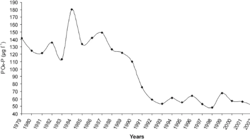
Fig. 1. Annual average of PO4-P load (µg L−1) in the Danube River at Nagytétény between 1979–2002 based on samples collected on a weekly basis.
Table 1. Summary of indicators used in the study. Along with average and total phytoplankton biomass (mg L−1) the table includes indicators for certain periods of a year presented as the order of sample within a year, i.e., sampling occasion within a year (on the average 49 samples per year were collected).
Symbol Indicator review Unit
b Annual total biomass: sum of phytoplankton biomass recorded throughout the year mg L−1 p Biomass peak: biomass peak observed within the year mg L−1 10% Occurrence of 10 %: the number of the sample within the year at which 10 % of annual
total biomass is reached
number of sample within a year 25% Occurrence of 25 %: the number of the sample within the year at which 25 % of annual
total biomass is reached
number of sample within a year 50% Occurrence of 50 %: the number of the sample within the year at which 50 % of annual
total biomass is reached
number of sample within a year Feb February:average phytoplankton biomass recorded in February mg L−1 Mar March:average phytoplankton biomass recorded in March mg L−1 Jul July:average phytoplankton biomass recorded in July mg L−1 Win Winter:average phytoplankton biomass recorded in winter (December, January, February) mg L−1 Spr Spring:average phytoplankton biomass recorded in spring (March, April, May) mg L−1 Sum Summer:average phytoplankton biomass recorded in summer (June, July, August) mg L−1
is best highlighted in PO4-P concentrations at the station of Nagytétény, seems to be the best evidence for that. Ac- cording to the data of the National Monitoring Network of the Environmental Authorities PO4-P load was consider- ably high till 1990, followed by considerably lower values from 1991 (Fig. 1).
Based on these observations, the value of nutrient ex- cess was taken into account upgrading the model fit.
The two submodels fitted to the data of 1979–1990 and 1991–2002, respectively, were run with the 24-year tempera- ture data (1979–2002) so as to being compared to each other statistically. The two submodels were validated by leaving out 1 year from each of them during the fitting. Degree of fitting was tested with correlation analysis by means of dif- ferent indices and indicators and accepted when correlation coefficient reached significant levels. In order to check fit- ting we took indices characterizing the 24-year long data as a whole, but they do not say anything about individual years. Such indices include correlations of monthly and sea- sonal averages of the 24 years. We defined indicators each of which assigns a number to individual years or certain periods of a year (Table 1), then, we analyzed the linear correlation of measured and simulated values.
These indicators needed improvement, and so we have developed 3 groups of indicators.
The first group includes indicators of yearly total biomass based on sum of phytoplankton biomass recorded throughout the year. The second group includes those of phenological ones, such as the number of the sample within the year at which 10% of yearly total biomass is reached re- ferred to as the “10%”indicator. Both “10%” and “25%”
indicators describe rapid phytoplankton development in spring, whereas “50%” indicator marks the period when 50%
of yearly total phytoplankton biomass is reached. “50%” in- dicator, at the same time, shows population development with two or more peaks within a year much better than does the occurrence of maximum biomass value within the year. The third group includes indicators of certain seasons and months.
Each period is characterized by the average of the phytoplankton biomass belonging to it. The average phy- toplankton biomass belonging to the winter (Win), spring (Spr) and summer (Sum) furthermore to the February (Feb), March (Mar) and July (Jul) periods were considered indicators. Regarding the autumn period the model did not show significant correlation.
Now, run the model with the different temperature data set (e. g. data of climate change scenarios and mea- sured – historical – data of temperatures) and those indica- tors can be of good applicability to contrast phytoplankton
biomass and phenology under various temperature regimes.
In this case study, the effect of linear temperature rise was analyzed: each value of the measured temperatures be- tween 1979 and 2002 was increased by 0.5, 1, 1.5 and 2◦C, respectively, then, the model was run with these data.
One-way ANOVA was applied to demonstrate possi- ble differences between model outcomes. In order to point out what groups do differ from the others, the post-hoc Tukey test was used, homogeneity of variance was tested with Levene’s test, when this assumption failed, Welch F- test was used. When evaluating the pairwise comparisons the Bonferroni- corrected Mann- Whitney test was also ap- plied besides the Turkey test, to consider any accidental correlations.
All statistical analyzes was performed with the Past software version 1.36 (Hammer et al. 2001).
Results
The DPGM
Linear combination of 21 theoretical populations re- sulted in the best fitting to measured phytoplankton biomass data as a whole. More than 500 species of planktonic algae have been recorded in the investi- gated reach of the Danube River (Kiss 2007; Kiss et al. 2007), so thus “theoretical populations” can be de- fined on the basis of the real species and their demand on temperature, respectively. Biomass (mg L−1) of a certain theoretical population at time “t” is the func- tion of its biomass measured a day before and the value of the temperature or light coefficient. A mini- mum function was used to determine whether temper- ature or light is the driving force behind population growth:
Ni,t = min(RT;RL)v·Ni,t−1+ 0.005
whereNi,trepresents biomass of theoretical population iat the timet,Ni,t−1represents biomass of the theoret- ical populationione day before timet,v is a factor of growth rate (species may differ in their growth rate), fi- nally, the constant of 0.005 means spore number (which was built into the model so as to prohibit extinction).
RT is function of temperature (growth rate depending on temperature, which can be described with the den- sity function of normal distribution), RLis growth rate depending on light. The latter can be described as fol- lows:
RL=a(1−
Ni/K)c
whereais maximal growth rate,Krepresents environ- mental sustainability implying for the effect of light.K forms a sine curve (Fig. 1).
K= 2.76×10−6·[4950000 sin(0.02t−1.4)+5049999]Kw where t is day of the year. We took into consideration the order of magnitude of difference between minimum and maximum biomass (Felf¨oldy 1981) and the finding that differences between summer and winter peaks can
Fig. 2. “K” – sine curve implying the effect of light presented in log scale (“Kw” works before day 50 and after day 295).
be as large as two orders of magnitude (V¨or¨os & Kiss 1985). The multiplier 2.76 × 10⁻⁶ was added to the formula so as to convert density into biomass. The value of 2.76×10⁻⁶is the result of optimization procedure.
The multiplier of Kw works only in the winter term (before the 50th and after the 295th day of the year), when algae utilize much less light due to the decreased angle of incidence (Felf¨oldy 1981). The modifier sine curve (Fig. 2) can be defined as follows:
Kw= 1.82 sin(0.02t−1.4) + 1.85
Finally, total phytoplankton biomass comes from the linear combination of individual theoretical species:
Nsum=
(ci·Ni)
wherecrepresents a species-specific constant multiplier, implying for function of ability of individual theoretical populations to utilize light and for the function of their size, respectively.
To launch the model some basic data is required, that is 0.01 mg L−1 algal biomass in 1979 January 1, then the model is run with data of temperatures considering light availability as well. In this way, us- ing 21 theoretical populations, the simulated patterns are in good accordance with measured biomass data within a year (Fig. 3). Simulation, however, does not indicate decreasing tendency of biomass within the monitoring period as was documented in the plank- ton record program. This becomes apparent when we look at the extreme values which the model cannot re- produce well, but the model underestimates biomass in the first half of the 24-year period as well. In the last 4 years, however, the model rather overestimates the biomass.
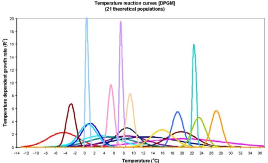
Temperature optimum curves of those 21 theoret- ical populations are presented in Fig. 4 and include 3 generalists with wide amplitude of temperature toler- ance, 3 specialists with narrow amplitude of tempera- ture tolerance and 15 transient ones.
Fig. 3. DPGM model fit: the observed and simulated values of phytoplankton biomass throughout the period of 1979–2002. Horizontal axis – number of sampling occasions conducted within the 24-year period; vertical axis – phytoplankton biomass (mg L−1).
Fig. 4. Temperature optimum curves of the 21 theoretical populations of DPGM.
The subdivision of DPGM into two submodels on the basis of two periods of different nutrient load:
DPGM-submodel A (DPGM-sA) and DPGM-submodel B (DPGM-sB)
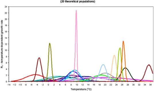
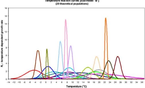
In order to eliminate shortcomings of DPGM, further environmental variables were taken into account. As- suming that high nutrient load means a specific envi- ronment for phytoplankton, two model versions were developed. One for the period of high nutrient excess in 1979–1990 (submodel “A”, DPGM-sA), and a second one for the period of lower nutrient excess in 1991–2002 (submodel “B”, DPGM-sB), both of which came about by combination of 20 theoretical populations.
The submodels were each fit on two different 11- year of temperature data, leaving out 1 year from both 12-year data series (1990 and 2002) to test and validate the model.
These two submodels differed slightly in the pa- rameters (mean, standard deviation) of temperature optimum curves (Figs 6, 7), remarkable differences were only in case of populations with narrow amplitude of temperature tolerance. Combination of DPGM-sA and DPGM-sB added up to the 24-year tactical model (Fig.
5).
DPGM-sA eliminated underestimation of biomass, and DPGM-sB ended biomass overestimation in the
Fig. 5. DPGB-sAB as a result of the combination of DPGM-sA and DPGM-sB. The last years of the two periods (1990 and 2002) are used for validation.
Fig. 6. Temperature optimum curves of the 20 theoretical species of DPGM-sA.
last four years (1999–2002). Combining the above- mentioned submodels into DPGB-sAB, we get a more realistic picture of phytoplankton biomass variation within the period of 1979–2002, and at the same time, the decreasing tendency of abundance becomes distinct.
Fit control
The decreasing trend of phytoplankton biomass within the period of 1979–2002 does not appear in the basic model version of DPGM (Fig. 8/A), however, it be- comes apparent in DPGM-sAB (Fig. 8/B).
Basic model version (DPGM) was not a good pre-
dictor of algal blooms (Fig. 8/A), DPGM-sAB, how- ever, showed much better figures (Fig. 8/B). The nor- mality of residuum is also better in case of DPGM-sAB, especially in case of low values (Figs 9/A and 9/B).
We propose DPGM-sAB as the final version of the DPGM model, which takes into consideration different levels of nutrient load within the study period.
In case of DPGM the correlation between field data and the data generated by the model is not strong enough (r= 0.57;p<0.01). In case of DPGM-sAB an improvement can be observed regarding the strength of the correlation (r= 0.62;p<0.01).
Fig. 7. Temperature optimum curves of the 20 theoretical species of DPGM-sB.
Fig. 8. Observed and simulated patterns of phytoplankton biomass on the basis of 15–day moving averages (trendlines are added):
DPGM (A) and DPGM-sAB (B).
Fig. 9. Normal probability plot for basic version of DPGM (A) and for DPGM-sAB (B).
Fig. 10. Linear correlation of simulated (DPGM-sAB) and measured data based on monthly (A) and seasonal averages (B).
Table 2. Observed and simulated means and standard deviations of indicators (listed in Table 1) on the basis of samples collected throughout 24 years, and correlation statistics (correlation coefficient, significance level), *sn = sequential number.
Observed DPGM-sAB Correlation
Indicators unit
mean st. dev. mean st. dev. r p
Annual total biomass mg L−1 606.3 214.2 592 128.9 0.6 <0.05
Biomass peak mg L−1 42.6 12.1 33 9.7 0.73 <0.05
Occurrence of 10 % sample sn* 10.7 2.4 10.3 2.7 0.59 <0.05
Occurrence of 25 % sample sn 15.2 3.1 15.6 3 0.6 <0.05
Occurrence of 50 % sample sn 22.7 3.7 23.9 2.7 0.58 <0.05
February mg L−1 5.2 5.4 6 4.8 0.7 <0.05
March mg L−1 15 10.6 12.2 7.7 0.81 <0.05
July mg L−1 17.8 11.5 21.6 9 0.66 <0.05
Winter mg L−1 31.5 35.9 37.1 21.7 0.78 <0.05
Spring mg L−1 239.5 93.8 198.5 64.4 0.67 <0.05
Summer mg L−1 219.9 111.2 251 88.8 0.61 <0.05
Because the indicators were created based on sea- sonal and monthly averages for the characterization of different intervals of the year, one can observe how the model correlates with the measured data from this point of view (Fig. 10/A). Based on these averages ten- dencies are more visible, because they are not disturbed to such an extent by the noise deriving from daily me- teorological factors and circumstances of sample collec- tion.
Observed and simulated biomass correlated signif-
icantly (r = 0.75; p <0.01) and this relationship was even more robust when seasonal averages were consid- ered (r= 0.79;p<0.01) (Fig. 10/B).
Indicators and their correlation analyzes
Summary of indicators, based on their means and stan- dard deviations within 24 years, is presented in Table 2.
Observed and simulated (with DPGM-sAB) patterns can be contrasted by use of indicators. Indicators of certain periods within a year, i.e. when phytoplankton
sA(0.5) – sB(0) *** *** *** * 1
sA(0.5) – sB(0.5) *** *** *** * 1
sA(0.5) – sB(1) *** *** *** * ** 1
sA(0.5) – sB(1.5) *** *** *** ** ***
sA(0.5) – sB(2) 1 *** *** *** ** 1 *** 1
sA(1) – sA(1.5) 1 1 1 1 1 1 1 1 1 1 1
sA(1) – sA(2) * * * 1 1 1 1 1 *
sA(1) – sB(0) *** *** *** * 1
sA(1) – sB(0.5) *** *** *** * 1
sA(1) – sB(1) *** *** *** * ** 1
sA(1) – sB(1.5) *** *** *** *** *** 1
sA(1) – sB(2) *** *** *** ** 1 *** 1
sA(1.5) – sA(2) * * * 1 1 1 1 1 *
sA(1.5) – sB(0) *** *** ** * 1
sA(1.5) – sB(0.5) *** *** *** * 1
sA(1.5) – sB(1) *** *** *** * ** 1
sA(1.5) – sB(1.5) *** *** *** ** *** 1
sA(1.5) – sB(2) *** *** *** * 1 ** 1
sA(2) – sB(0) *** *** *** *** *** * 1 ***
sA(2) – sB(0.5) *** *** *** *** *** * 1 ***
sA(2) – sB(1) *** *** *** *** *** * * 1 ***
sA(2) – sB(1.5) *** *** *** *** *** * * ** 1 ***
sA(2) – sB(2) *** *** *** *** *** * 1 * ** ***
sB(0) – sB(0.5) 1 1 1 1 1 1 1 1 1 1 1
sB(0) – sB(1) 1 1 1 1 1 1 1 1 1 1 1
sB(0) – sB(1.5) 1 1 1 1 1 1 1 1
sB(0) – sB(2) 1 1 1 1 1 1 1 1 1 1
sB(0.5) – sB(1) 1 1 1 1 1 1 1 1 1 1 1
sB(0.5) – sB(1.5) 1 1 1 1 1 1 1 1 1
sB(0.5) – sB(2) 1 1 1 1 1 1 1 1 1 1
sB(1) – sB(1.5) 1 1 1 1 1 1 1 1 1 1 1
sB(1) – sB(2) 1 1 1 1 1 1 1 1 1 1 1
sB(1.5) – sB(2) 1 1 1 1 1 1 1 1 1 1
Significant differences are marked with asterisk, high similarities (0.99<p<1) are marked with 1.*p<0.05; **p<0.01; ***p<0.001
production reaches 10%, 25%, and 50% of its yearly maximum, were defined with the sequential number of sample within the 24-year record. On the average, 49 samples were collected within a year. Yearly total biomass was calculated by the sum of biomass measured in individual samples throughout the year. Results in- dicated that 10% of yearly total biomass is reached in the second half of March, whereas 25% limit is reached between middle of April-beginning of May, and 50% in June, respectively. Table 2 presents correlation coeffi- cients and results of statistical analysis per indicator.
Effect of linear temperature rise
One-way ANOVA detected strong significant varia- tion among and within submodels at most indicators (p <0.001), except for two of them. Indicator “Mar”
(March) and “Spr” (Spring) did not show any signif-
icant variation (p > 0.05). Homogeneity of variance is obtained only in case of “50%”, “Feb”, “Mar” and
“Spr” indicators (Levene’s test, p > 0.05). Based on the findings of Welch F-test, standard deviations dis- played major differences at most indicators (p<0.001), in case of “Mar” 0.001<p<0.01. Only indicator “Spr”
(Spring) did not show any variation (p>0.05).
Tukey’s pairwise comparisons (Table 3) suggest that most indicators show larger variation among sub- models compared with those of linear temperature rise within a submodel. DPGM-sB shows high homogeneity, so, we can conclude that warming has no considerable effect here. This is also supported by the results of the Bonferroni-corrected Mann-Whitney test (Table 4).
A number of indicators implied larger variation among submodels rather than within a submodel with different input data of temperatures. Such indicators
Table 4. Results of Mann-Whitney pairwise comparison (Bonferroni, corrected) among and within submodels at different levels of temperature rise. “sA” and “sB” represent DPGM-sA and DPGM-sB, respectively, level of linear temperature rise (◦C) is indicated in parentheses.
b p 10% 25% 50% Feb Mar Jul Win Spr Sum
sA(0) – sA(0.5)
sA(0) – sA(1) 1
sA(0) – sA(1.5)
sA(0) – sA(2) *** *** ** * ***
sA(0) – sB(0) *** *** *** *** *** *** *** ***
sA(0) – sB(0.5) *** *** *** *** *** *** *** ***
sA(0) – sB(1) *** *** *** *** *** *** *** ***
sA(0) – sB(1.5) *** *** *** *** *** *** *** ***
sA(0) – sB(2) *** *** *** *** *** *** *** ***
sA(0.5) – sA(1) sA(0.5) – sA(1.5)
sA(0.5) – sA(2) *** ** * ***
sA(0.5) – sB(0) *** *** *** *** *** * *** *** 1 ***
sA(0.5) – sB(0.5) *** *** *** *** *** * ** *** ***
sA(0.5) – sB(1) *** *** *** *** *** * ** *** ***
sA(0.5) – sB(1.5) *** *** *** *** *** * ** *** ***
sA(0.5) – sB(2) *** *** *** *** *** *** *** ***
sA(1) – sA(1.5)
sA(1) – sA(2) ** * 1 *
sA(1) – sB(0) *** *** *** *** *** *** *** *** ***
sA(1) – sB(0.5) *** *** *** *** *** *** *** *** ***
sA(1) – sB(1) *** *** *** *** *** ** *** *** ***
sA(1) – sB(1.5) *** *** *** *** *** ** *** *** ***
sA(1) – sB(2) *** *** *** *** *** * *** *** ***
sA(1.5) – sA(2) ** * *
sA(1.5) – sB(0) *** * *** *** *** *** ** *** *** ***
sA(1.5) – sB(0.5) *** *** *** *** *** * *** *** ***
sA(1.5) – sB(1) *** *** *** *** *** * *** *** ***
sA(1.5) – sB(1.5) *** *** *** *** *** * *** *** ***
sA(1.5) – sB(2) *** *** *** *** *** *** *** ***
sA(2) – sB(0) *** *** *** *** *** ** *** *** ***
sA(2) – sB(0.5) *** *** *** *** *** *** ** *** *** ***
sA(2) – sB(1) *** *** *** *** *** *** ** *** *** ***
sA(2) – sB(1.5) *** *** *** *** *** *** ** *** *** ***
sA(2) – sB(2) *** *** *** *** *** *** *** *** ***
sB(0) – sB(0.5) 1 1
sB(0) – sB(1) sB(0) – sB(1.5) sB(0) – sB(2) sB(0.5) – sB(1)
sB(0.5) – sB(1.5) 1
sB(0.5) – sB(2) sB(1) – sB(1.5)
sB(1) – sB(2) 1
sB(1.5) – sB(2)
Significant differences are marked with asterisk, high similarities (0.99<p<1) are marked with 1. *p<0.05; **p<0.01; ***p<0.001
include 10%, 25%, 50%, and Win, in most levels of tem- perature rise. This phenomenon can be observed more efficiently in the results of the Bonferroni-corrected Mann-Whitney test, in which there are major differ- ences between the two submodels in case of indicators b and p.
The effect of linear temperature rise becomes ap- parent at DPGM-sA in case of high temperature rise.
This is realized through variation in biomass within submodel-A including indicators of biomass measure (b, p), and summer biomass (Sum). Here, in response to a temperature rise of 2◦C, output of DPGM-sA differs significantly from those of other data in most cases. In the springtime (Mar, Spr) there cannot be expected any changes as a consequence of climate change, in case of either of the submodels and either of the indicators.
Table 5/A-B suggests that biomass increases with rising temperatures explicitly (b; in case of DPGM-sA).
The most significant growth was experienced when the temperature was increased by 2◦C. Maximum values of monthly biomass (p) increase as well, however, standard deviations are also quite apparent. One expects similar outcomes in summer (Sum), particularly in July (Jul):
an increasing biomass with the rising of temperature, especially in case of a 2◦C temperature rise. Considering the total annual biomass (b) and the biomass quanti- ties measured during the period of maximum produc- tion (Jul, Sum), one can also notice that in the case of lower (0.5◦C) temperature rise, the biomass increases only to a smaller extent as well, however, the standard deviations increase in a larger measure: this means that there can be expected a major variation between years.
Sum 31.9 42.6 47.8 48.8 93.6 15.6 15.6 15.6 15.8 15.7
B DPGM-sA DPGM-sB
0 0.5 1 1.5 2 0 0.5 1 1.5 2
b 3137.5 7246.2 5710.4 4214.4 8054.9 463.0 487.2 625.5 736.6 613.8
p 2117.4 3484.6 4392.1 3956.6 5839.0 134.5 230.6 245.4 312.3 349.3
10% 13.1 21.8 23.4 27.6 41.0 7.4 9.7 11.8 13.3 11.2
25% 22.2 18.1 17.8 26.3 32.2 13.0 15.1 16.3 19.8 15.5
50% 18.6 16.7 14.1 12.9 17.2 13.5 16.8 18.5 21.8 16.5
Feb 2.1 2.2 2.3 2.2 2.9 2.9 3.4 4.6 9.1 8.2
Mar 25.8 5.1 4.0 4.2 3.4 5.6 9.6 7.7 8.0 4.2
Jul 12.2 241.8 167.9 126.1 261.7 3.5 4.4 4.3 5.0 4.3
Win 0.9 0.9 0.9 0.9 1.0 1.0 1.2 1.5 3.1 2.8
Spr 9.4 4.0 3.8 3.8 7.4 3.4 4.5 6.7 7.3 5.4
Sum 30.0 78.9 60.9 46.2 90.9 1.9 2.2 2.8 3.7 3.6
A dramatic (2◦C) temperature rise already results in a definite, large-scale biomass growth.
Rising temperatures cause a positive shift, i.e. shift towards posterior peaks, in development of algal popu- lations at which 10% of yearly total biomass is reached.
This trend emerges at “25%” again albeit less definitely, however, in case of “50%” there is no remarkable shift.
Discussion
The case study of DPGM model pointed out that vari- ation of phytoplankton biomass within and over years can be simulated through consideration of daily temper- ature as well as light availability. Generally, the model estimates biomass variation within years quite well, however, underestimation of phytoplankton biomass in early years and overestimation in the last four years – the extent of which lags behind those of the underes- timations in the early years – suggest drastic change in environmental variables beyond temperature over the study period. Although mean water temperature in the Danube River experienced some variation over the study period, no remarkable increase was demon- strated (Tóth 2007), whereas discharge peaks reported over 4–6-year cycles increased to a certain degree (Ve- rasztó et al. 2010). The trend in phytoplankton biomass variation over the study period, however, cannot be at- tributed to those observations.
Generally, nutrients have been considered when seasonal dynamics of phytoplankton is discussed even if global warming-related effects are in the primary fo-
cus of research (e. g. Mooij et al 2007; Malmaeus &
H˚akanson 2004; Hassen et al. 1998; Komatsu et al.
2006). We did not consider nutrients within the DPGM model because inorganic nutrients have not been found as limiting factors in the Danube River – similarly to large rivers – as they do in lakes. In reality, availability of light has been found to limit algal growth rather than nutrients, the oversupply of which has been reported in the Danube River (Kiss 1994, 1996). The marked in- crease of algal biomass in the 70’s can be attributed to the altering light conditions of the river because nu- trient supply of the 50’s and 60’s had the capacity to create a trophic status similar to those of recent years (Kiss 1994). Only light conditions and their major al- tering force, the amount of suspended matter, have ex- perienced remarkable variation since the middle of 60’s due to the increasing constructions of dams. Reservoirs have decreased velocities and, therefore, some portion of suspended sediments became settled. As a result of those, the amount of suspended matter decreased by the end of the 70’s and light conditions improved im- plicitly, which contributed to a significant increase in algal individual numbers (Kiss 1994; Kiss & Genkal 1996). From the 90’s, light conditions have not exhib- ited profound variation, in addition, nutrient oversup- ply decreased (Horváth & Tevanné-Bartalis 1999; Varga et al. 1989), which might account for decreased algal biomass. However, the degree of nutrient excess may de- termine the potential maximum biomass of algae, thus after all, we expect long-term change in nutrient load to affect phytoplankton biomass in the Danube River.
Consequently, we propose that, among unidentified en- vironmental variables, degree of nutrient load is the ma- jor cause behind extreme peaks and decreasing trend of phytoplankton biomass. Theoretically, increasing re- lease of inhibitors of algal growth, or other human pol- lutants may account for decreased algal biomass as was documented in some case studies (Barinova et al. 2008) however, long-term record of water chemical variables in the Danube River does not indicate such profound variation (Tóth 2007). Another rational assumption in- cludes variation in discharge, which can have profound effect on phytoplankton biomass development (Kiss &
Schmidt 1998), although discharge variation during the study period does not imply such trend as was ob- served in algal biomass (Verasztó et al. 2010), thus, discharge variation cannot serve as a true predictor of algal biomass.
On the basis of long-term water chemical data, variation in nutrient load (expressed in PO4-P con- centration) can answer the question discussed above.
Results of temporal coenological patterns constructed from phytoplankton database supported this scenario (Verasztó et al. 2010), where change in phosphorus load goes hand in hand with phytoplankton clusters in or- dination plot. Assuming that high level of nutrient ex- cess serves a different kind of environment for algae than does low level of nutrient oversupply, purely tem- perature variation improves simulation of algal biomass without building a nutrient variable into the model. Re- sults suggest that different levels of nutrient oversupply (characterized with PO4-P concentration) create differ- ent environments to phytoplankton, and – according to those levels of oversupply – algae display different dy- namics in answer to global warming.
The apparent “breakpoint” of the study period in 1990 coincides with the economic and environmental consequences of regime shift in Hungary, one of the most important historical episode of the country. At that time, the collapse of socialist industry brought into a significant decrease of local pollutants released into the river. At a guess, in the Danube catchment, nutrient load decreased by 40–50% due to the over- all economic recession and rapid development of sew- erage/wastewater treatment following the regime shift (Schreiber et al. 2005; ICPDR 2005; Csathó et al. 2007).
Not surprising, extreme phytoplankton peaks of short development were observed within that period suppos- ing rapid nutrient load. DPGM model forecasts biomass peaks after the regime shift through considering purely temperatures. Only in case of two extreme peaks were the multiplier added so as to taking nutrient load into account as well. Those events both occurred in 1992 and were not the highest biomass values recorded after 1990.
Simulated biomass (DPGM-sAB) showed signifi- cant correlation with measured biomass regarding three indicator groups of different types. In the field of cli- mate change research, defining indicators is of absolute necessity (Diós et al 2009). The indicators presented above are of good applicability even when we run the
model with the data of climate change scenarios.
By distinguishing two different periods of nutri- ent load, the validated DPGM-sAB is able to simulate phytoplankton biomass variation on the basis of daily temperatures as input, negligible failure occurs though.
With this in mind, the model can be capable of fore- casting possible future states of algal assemblages in the Danube River by use of temperature data of cli- mate change scenarios. Input parameters include only daily air temperatures, there is no need for further data of daily frequency. Modeling studies face the problems of lack of data and access to them, respectively (Porter et al. 2005), which are really true for climate change- related modeling (Sipkay et al. 2009b). On the one hand, data that have been gathered elsewhere are often difficult to obtain, on the other hand, long-term data of different water bodies have often been collected with different methodologies. What is more, complex models require a number of data that have not been measured yet. In most cases, this is the reason behind lack of ap- plication of model systems, describing the general func- tioning of the system, in a number of aquatic habitats in the limelight. Thus, the presented tactical model, de- scribing the seasonal dynamics of phytoplankton of the Danube River on the basis of daily temperatures, is rel- atively simply and fruitful to be adapted for climate change research.
Linear temperature rise has remarkable effects on phytoplankton biomass only in case of high level of nu- trient load, particularly in the summer term of high algal production. When nutrient overload reaches low levels, temperature rise does not create significant vari- ation in phytoplankton dynamics as was demonstrated through the examples of indicators. With this end in view, it can be concluded that degree of nutrient load is of major importance when global warming is consid- ered. In addition, global warming brings more drastic change to ecosystems of high nutrient load. All these draw attention to the increasing hazard of nutrient load in rivers.
Indicators implied major variation between DPGM- sA and DPGM-sB. In case of DPGM-sA (assuming higher level of nutrient load) higher biomass are de- tected, and the timing of the initial phytoplankton growth are later than in case of DPGM-sB.
DPGM-sA responds more strongly to climate change, as a consequence of which the algae commu- nity of this model starts developing later, however, it reaches an immensely high biomass by summertime. In relation to the alteration of timing it would be reason- able to expect that the development of phytoplankton begins earlier as a consequence of climate change, never- theless we experience the opposite. Based on indicators characterizing the spring period, one shall not expect any alteration in this season. Although the growth of biomass during summertime can be dramatic. Should this scenario be met, after an intensive rise similar to the recent one, in the springtime, a much more inten- sive increase can be expected to begin in the summer period characterized by very high temperatures, ap-
mums to occur earlier within the year, particularly in the winter half-year (Thackeray et al. 2008).
Global warming may have fundamental effects on the trophic status and primary production of inland waters (Lofgren 2002). Bacterial metabolism, rate of nutrient cycling and biomass increase of phytoplankton abundance all increase with rising temperatures (Klap- per 1991), albeit some studies have found algal biomass to decrease with rising temperatures (Lewandowska
& Sommer 2010; Sommer & Lengfellner 2008). As a general rule, climate change connected with human- derived pollution enhances eutrophication (Klapper 1991; Adrian et al. 1995). While changes in species com- position may be complex and unpredictable, an overall increase in system productivity is likely to be a common response to climate warming. Climate change will inter- act with other threats to lotic ecosystems, enhancing some regional water shortages, favoring species inva- sions, and acting as an additional stressor on the biota (Allan & Castillo 2007). In the assessment of ecologi- cal changes attributed to global warming, we have to consider trophic state and morphology of inland waters (Anneville et al. 2010). A number of authors adopt- ing modeling methodologies have forecasted increase of phytoplankton abundance under increasing tempera- tures mostly through rising trophity (Mooij et al. 2007;
Elliot et al. 2005; Komatsu et al. 2006). These findings correspond with our results of linear temperature rise, but only in those particular cases of high nutrient load.
Present study suggests that, in case of low level nutrient load, rise in temperature does not have such a remark- able effect on phytoplankton biomass as does tempera- ture rise along with high nutrient availability. Assuming higher level of nutrient load the phytoplankton biomass rising is drastic due to the warming, without changes in phosphorus load. Consequently if the nutrient load is also rising, the changes in Danubian phytoplankton biomass will be dramatic.
Acknowledgements
Our research was supported by the research proposal OTKA TS 049875 (Hungarian Scientific Research Fund); the VA- HAVA project; the KLIMA-KKT project (National Office for Research and Technology, Ányos Jedlik Programme); the Adaptation to Climate Change Research Group (Hungarian Academy of Sciences, Office for Subsidized Research Units);
Function of Running Waters. Second edition. Springer, The Netherlands
Andersen H.E., Kronvang B., Larsen S.E., Hoffmann C.C., Jensen T.S. & Rasmussen E.K. 2006. Climate-change impacts on hy- drology and nutrients in a Danish lowland river basin. Science Total Environ.365:223–237.
Anneville O., Molinero J.C., Souissi S. & Gerdeaux D. 2010. Sea- sonal and interannual variability of cladoceran communities in two peri-alpin lakes: uncoupled response to the 2003 heat wave. J. Plankton Res.32(6):913–925.
Barinova S., Medvedeva L. & Nevo E. 2008. Regional influ- ences on algal biodiversity in two polluted rivers (Rudnaya River, Russia, and Quishon River, Israel) by bioindication and canonical correspondence analysis. Applied Ecol. Envi- ron. Res.6(4):29–59.
Behrendt H., Van Gils J., Schreiber H. & Zessner M. 2005. Point and diffuse nutrient emissions and loads in the transboundary Danube River Basin. – II. Long-term changes. Large Rivers 16/1–2. Arch. Hydrobiol. Suppl.158(1–2):221–247.
Blenckner T., Omstedt A. & Rummukainen M. 2002. A Swedish case study of contemporary and possible future consequences of climate change on lake function. Aquatic Sci.64(2):171–
184.
Csathó P., Sisák I., Radimszky L., Lushaj S., Spiegel H., Nikolova M.T., Nikolov N. Čermák P., Klir J., Astover A., Karklins A., Lazauskas S., Kopi´nski J., Hera C., Dumitru E., Manojlovic, M., Bogdanovi´c D., Torma S., Leskošek M. & Khristenko A.
2007. Agriculture as a source of phosphorus causing eutroph- ication in Centra and Eastern Europe. British Society of Soil Science Suppl.23:36–56.
Déri A. 1991. The role of nitrification the oxygen depletion of the River Danube. Verh. Internat.Verein.Limnol.24:1965–1968.
Diós N., Szenteleki K., Ferenczy A., Petrányi G. & Hufnagel, L.
2009. A climate profile indicator based comparative analysis of climate change scenarios with regard to maize (Zea mays L) culures. Appl. Ecol. Environ. Res.7(3):199–214.
Drégelyi-Kiss Á., Drégelyi-Kiss G. & Hufnagel L. 2008. Ecosys- tems as climate controllers – biotic feedbacks (a review).
Appl. Ecol. Environ. Res.6(2):111–135.
Drégelyi-Kiss Á & Hufnagel L. 2009a. Simulations of Theoretical Ecosystem Growth Model (TEGM) during various climate conditions. Appl. Ecol. Environ. Res.7(1):71–78.
Drégelyi-Kiss Á. & Hufnagel L. 2009b. Effects of temperature- climate patterns on the production of some competitive species on grounds of modeling. Environ. Model. Assessm.
15(5):369–380.
Elliott J.A., Thackeray S.J., Huntingford C. & Jones R.G. 2005.
Combining a regional climate model with a phytoplankton community model to predict future changes in phytoplankton in lakes. Freshwater Biol.50:1404–1411.
Felf¨oldy L. 1981. A vizek k¨ornyezettana.Általános hidrobiológia.
Mez˝ogazdasági Kiadó, Budapest.
Flanagan K.M., McCauley E., Wrona F. & Prowse T. 2003. Cli- mate change: the potential for latitudinal effects on algal biomass in aquatic ecosystems. Can. J. Fish Aquat. Sci.60:
635–639.