Stability Analysis and Control of Hybrid Systems
PhD thesis
Written by: Szabolcs Rozgonyi Supervisor: Prof. Katalin Hangos
University of Pannonia
Doctoral School of Information Science and Technology
2011
Stability Analysis and Control of Hybrid Systems
Értekezés doktori (PhD) fokozat elnyerése érdekében
Írta:
Rozgonyi Szabolcs
Készült a Pannon Egyetem Informatikai Tudományok Doktori Iskolája keretében Témavezet®: Dr. Hangos Katalin
Elfogadásra javaslom (igen / nem)
(aláírás) A jelölt a doktori szigorlaton ...%-ot ért el
Veszprém, ...
a Szigorlati Bizottság elnöke Az értekezést bírálóként elfogadásra javaslom:
Bíráló neve: ... (igen / nem)
(aláírás)
Bíráló neve: ... (igen / nem)
(aláírás)
A jelölt az értekezés nyilvános vitájában ...%-ot ért el
Veszprém, ...
a Bíráló Bizottság elnöke
A doktori (PhD) oklevél min®sítése ...
...
Az EDT elnöke
Tartalmi kivonat
Napjainkban mind az elméleti területek kutatóitól, mind a gyakorlati alkalmazásokkal foglalkozó szakemberek részér®l egyre nagyobb gyelmet kap a hibrid rendszerek kontroll-elmélete, illetve ezen rendszerek stabilitásvizsgálata.
Jelen disszertációban egy módszert adunk nemlineáris rendszerek (beleértve a tartományonként deniált hibrid rendszerek) vonzási tartományának (domain of attraction, DOA) becslésére. A módszer Vanelli és Vidyasagar maximális Ljapunov-függvényeken alapuló algoritmusának javított változatán alapul.
A bemutatott algoritmust demonstráljuk egy iparilag releváns esettanulmányon, nevezetesen a Paksi Atomer®m¶ két részrendszerének stabilitásvizsgálatán keresztül. A rendszerek egyensúlyi pontjának vonzási tartományát vizsgáljuk az els® esetben a neutron-uxus, a második esetben pedig a szekunder kör g®zfejleszt®jének visszacsatolási tényez®jének függvényében.
A disszertáció további eredménye, hogy a Vanelli-Vidyasagar algoritmust kiterjeszti hibrid rend- szerek egy bizonyos osztályára a tartományonként deniált nemlineáris rendszerekre, melyet pél- dával is illusztrál. A reaktor primer körének hibrid modellje vonzási tartománya tisztán analitikus eszközökkel kerül meghatározásra, továbbá az egyensúlyi ponthoz történ® konvergencia sebességét is vizsgáljuk a visszacsatolási tényez®k különböz® értékeire.
Végül a disszertációban egy input-diszkrét hibrid rendszerhez, a reaktor nyomáskiegyenlít® tar- tályához tervezünk egy szabályozót több-paraméteres programozási technikával (MPT). Vizsgáljuk a kontrollertervezés több paraméterének hatását az eredményül kapott szabályozó bonyolultságára, illetve hatékonyságára.
Abstract
Stability analysis and control of physical systems that exhibit discrete-continuous hybrid behaviour are gaining increasing attention recently from both theoretical and practical perspectives.
A method is presented in this dissertation to nd an estimation for the domain of attraction (DOA) of non-linear systems including piecewise-dened hybrid systems. The method is based on a corrected version of the Vanelli-Vidyasagar-algorithm that uses maximal Lyapunov-functions.
The presented algorithm has been used for an industrially relevant case-study, for the stability analysis of two subsystems of the nuclear reactor in Paks Nuclear Power Plant. In the case of the rst subsystem the dependence of stability of the controlled neutron-ux on a feedback gain has been investigated. In the case of the second one the eect of the feedback gain on the DOA of the secondary circuit steam generator was analysed.
Furthermore, the Vanelli-Vidyasagar algorithm has also been extended in this dissertation to a class of hybrid systems, which has been demonstrated on an example, too. Moreover, the analytical construction of the DOA of the hybrid model of the primary circuit in the same power plant is also discussed. The analysis is done analytically, and the eect of feedback gains on the dynamics has also been investigated.
Finally a controller has been designed for an input-discrete hybrid system (the pressurizer tank of the reactor) using multi-parametric programming techniques. The eect of certain parameters of the controller design process is also investigated on the quality and on the complexity of the resulting controller.
Zusammenfassung
Die Stabilitätsanalyse und die Kontrolle von physikalischen Systemen mit diskret-kontinuierlichem Hybrid-Verhalten gewinnen zunehmend an Interesse, sowohl unter theoretischen als auch prakti- schen Aspekten.
In dieser Dissertation wird eine Methode zur Abschätzung des Anziehungsbereiches (Domain of Attraction / DOA) von nicht-linearen Systemen einschliesslich stückweise denierter Hybrid- systeme vorgestellt. Der Ansatz basiert auf einer korrigierten Version des Vanelli-Vidyasagar- Algorithmus unter Benutzung maximaler Lyapunow Funktionen.
Der vorgestellte Algorithmus ndet Anwendung in einer industriell relevanten Fallstudie: die Stabilitätsanalyse zweier Subsysteme des Kernreaktors der Paks Nuklearstromanlage. Im Falle des ersten Subsystems wird die Abhängigkeit der Stabilität eines kontrollierten Neutronenusses durch eine Rückkopplungsregelung untersucht. Für das zweite Subsystem wird der Eekt der Rückkopplungsregelung auf die DOA des Sekundärkreislaufs des Dampfgenerators analysiert.
Darüberhinaus wird der Vanelli-Vidyasagar-Algorithmus in dieser Dissertation auf eine Klasse von Hybridsystemen erweitert und anhand eines Beispiels erläutert. Ausserdem wird die analy- tische Konstruktion der DOA des Hybridmodels des Primärkreislaufs des genannten Kraftwerks diskutiert. Die Durchführung der Analyse erfolgt analytisch, wobei die Eekte der Rückkopplungs- regelung auf die Dynamik ebenfalls betrachtet werden.
Abschliessend folgt die Darstellung eines Reglers für ein Input-diskretes Hybridsystem (der Drucktank des Reaktors) mittels der Multi-Parametric Programmiertechnik. Der Einuss verschie- dener Parameter im Regler-Design-Prozess auf die Qualität und die Komplexität des resultierenden Reglers ist Gegenstand weiterer Untersuchungen.
Acknowledgement
I would like to express my gratitude to Dr. Katalin Hangos, my supervisor, for her invaluable help.
She gave me lots of advice and guidance in my research, helped me in my studies, and gave me inspiration when I was about to lose my enthusiasm.
I would also like to thank Gábor Szederkényi for his help over the years of my studies.
My gratitude could not even be expressed to my mother, Ágnes Balogh, who raised me up, selessly supported me over my childhood and as a young adult. Without her I would not be the same person as I am today. This work is dedicated to her.
I also want to thank my wife, Orsolya Serf®z® Rozgonyiné, for her love. The patience and support cannot be overestimated she provided to me which was necessary to nish this work.
I am also thankful for my previous employer Continental Teves Hungary Ltd. for providing the possibility to work on my PhD and also for Tellus Research Foundation for their support.
Furthermore my research work has been partially supported by the Hungarian Scientic Research Fund through grant no. K67625.
Contents
1 Introduction 11
1.1 Background and motivation . . . 11
1.2 Problem statement and aims . . . 12
1.3 The structure of the thesis . . . 12
1.4 Notations . . . 13
2 Basic notions and literature review 14 2.1 Basic notions on nonlinear autonomous systems and their stability . . . 14
2.1.1 Maximal Lyapunov functions . . . 16
2.2 Basic notions on hybrid systems and their stability . . . 18
2.2.1 Domain of attraction of piecewise hybrid nonlinear systems . . . 18
2.3 Controller design by multi-parametric programming . . . 19
2.3.1 Multi-parametric programs and their properties . . . 20
2.4 Nonlinear dynamic model of pressurized water reactor systems . . . 22
2.4.1 Stability analysis of nuclear system models . . . 23
2.4.2 Modelling assumptions . . . 23
2.4.3 Conservation balances . . . 24
2.4.4 Algebraic constitutive equations . . . 26
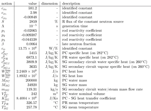
2.4.5 Constants . . . 27
3 Estimation of DOA of nonlinear autonomous systems 28 3.1 Improved estimation method of DOA for nonlinear autonomous systems . . . 28
3.1.1 The Vanelli-Vidyasagar algorithm . . . 28
3.1.2 Steps of the algorithm . . . 32
3.1.3 An uni-variable example . . . 33
3.2 Estimation of the DOA of a controlled pressurized water reactor . . . 34
3.2.1 The eect of feedback of the neutron ux (N) on the DOA . . . 34
3.2.2 Feedback of the secondary circuit liquid temperature of the steam generator (TSG) . . . 39
3.3 Summary . . . 41
4 Estimation of DOA of hybrid nonlinear systems 45 4.1 Extending Vanelli-Vidyasagar algorithm to piecewise hybrid systems . . . 45
4.1.1 The considered hybrid systems and their properties . . . 45
4.1.2 Finding the widest possible sub-level set . . . 46
4.1.3 DOA of a hybrid van der Pol system . . . 46
4.2 Determination of the DOA for the hybrid reactor model . . . 48
4.2.1 The investigated low dimensional primary circuit model . . . 48
Conservation balances . . . 49
Algebraic constitutive equations . . . 49
4.2.2 DOA of the hybrid reactor model . . . 50
Hybrid mode 1 . . . 50
Hybrid mode 2 . . . 52
4.2.3 Constructing the overall DOA in a second order hybrid case . . . 53
4.2.4 Analysis of the dynamics . . . 53
4.3 Summary . . . 53
5 Application of multi-parametric programming to controller design for discrete input hybrid nonlinear systems 56 5.1 Hybrid model of the vaporizer . . . 56
5.1.1 System description . . . 56
5.1.2 Conservation balances . . . 57
5.1.3 State-space model . . . 58
5.1.4 Hybrid states . . . 59
5.2 Controller design . . . 59
5.2.1 Controller performance evaluation . . . 60
5.3 Summary . . . 62
6 Conclusions 66 6.1 New results . . . 66
6.2 Future work . . . 67
6.3 Own publications . . . 68
A Appendix 74 A.1 The Mathematica package . . . 74
List of Figures
2.1 Controlled hybrid system . . . 20
2.2 MPC online optimization . . . 21
2.3 Process ow-sheet with the operating units of the simplied model . . . 25
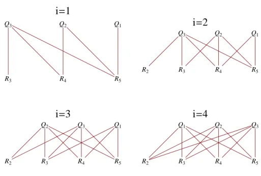
3.1 Pairs of Qiand Ri which should be multiplied in Eq. (3.22) form= 5 . . . 32
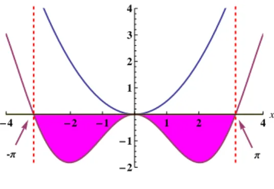
3.2 Stable segments (in red) of system (3.25) . . . 33
3.3 Solutions of system (3.25) . . . 33
3.4 The DOA of system (3.25) . . . 34
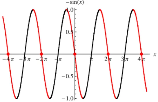
3.5 Structure of the neutron-ux dNdt =fN(N, v) . . . 35
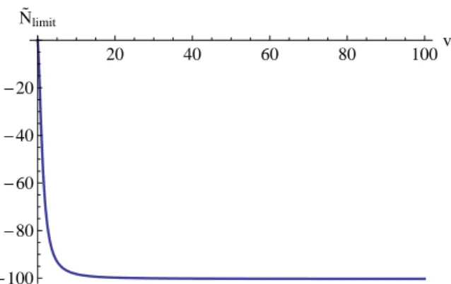
3.6 Dependence of limit N˜limit(v)onv . . . 36
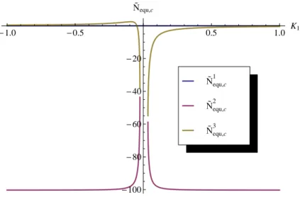
3.7 Dependence of controlled (and centred) neutron-ux equilibrium on feedback gainK1 37 3.8 Area of conditionPm−2 i=1 Qi(x)>−1 for dierent values ofK1's . . . 38
3.9 DOA of the closed loop subsystem of the neutron ux . . . 39
3.10 Dependence of eigenvaluesJ on gain factorK2 . . . 41
3.11 DOA of the controlled reactor in operation mode of T for several gainsK2. . . . 42
3.12 DOA of the controlled system for the caseK2= 0.1 . . . 43
3.13 DOA of the controlled system for the caseK2= 0.5 . . . 43
4.1 Trajectories of system (4.2) where the dash-dotted curve is the border between dynamicsX1 andX2 . . . 48
4.2 Estimated DOA for the hybrid van der Pol system . . . 49
4.3 Trajectories of the hybrid system, where the dark region shows mode 1, the light region corresponds to mode 2 . . . 51
4.4 Structure of the hybrid system. Dark green area shows the domain of hybrid mode 1, light green area shows the DOI. . . 52
4.5 Map of convergence speeds for dierent values ofKP R (WR= 3.5×10⁷) . . . 54
5.1 Simplied ow-sheet of the vaporizer . . . 57
5.2 Number of polytopes (Z) of the controller in function of sampling time (τ) and length of horizon (N) . . . 62
5.3 Operation of the controller forτ= 60,N = 4for dierent norms . . . 63
5.4 Operation of the controller forτ= 20,N = 5 . . . 63
5.5 Operation of the controller forτ= 30,N = 5 . . . 63
5.6 Operation of the controller forτ= 60,N = 3 . . . 64
5.7 Operation of the controller forτ= 60,N = 4 . . . 64
5.8 Partitions of the investigated controllers . . . 64
5.9 Trajectories of the controlled system . . . 65
List of Tables
2.1 Constants in the model equations . . . 27 3.1 Values ofPs for several gainsK1 . . . 38 5.1 Model parameters . . . 58
Chapter 1
Introduction
Everything that has been discovered in a given domain is almost nothing compared with what is left to be discovered!
Ramón y Cajal
1.1 Background and motivation
Modelling of physical systems is of vital importance both in areas of theoretical research and in industrial applications. System models are usually developed either to understand (analyse) or control (synthesise). The ones used in industry are often based on, or originated from rst engineering principles, see [1].
Models of physical systems can be described using various tools including linear or nonlinear approaches. The number of nonlinear representations is countless and currently it is practically hopeless to nd universal analytical techniques which are applicable to any nonlinear system with arbitrary input signal. Among the existing tools, however, one of the most important type of description is the representation by ordinary dierential equations.
Many applications demand, in addition, the ability of expressing a sort of discrete switching behaviour: while in nature nonlinearity is the rule rather than the exception, the same is true for being hybrid system among industrial applications. Hybrid systems are dynamic systems that exhibit both continuous and discrete dynamic behaviour, i.e., systems that can both ow (described by dierential equations) and jump (described by dierence equations or control graphs).
There are two fundamentally dierent ways of describing a hybrid system that possesses both continuous and discrete variables. The rst one utilizes the concepts of theory of discrete event systems (see [2], [3]) and embeds the continuous elements into a discrete system model. The other one is called switched systems approach, when some non-smooth variables are embedded into the continuous part (see [3]) in which the dynamics can be described by piecewise functions which are continuous, but not necessarily dierentiable on the border between dierent dynamics. There also exists an extended approach called systems with impulse eect (see [4, 5]) where the possibility is added to the states to jump when certain conditions are satised, often when some boundaries are crossed by the trajectory. These boundaries are general subsets of the state-space, often being described by zeros of several functions.
Dierent denitions of hybrid systems are analysed for example in [6] or [7].
Appearance of hybrid systems ranges from nuclear reactors [8], to automotive applications [9, 10] or even in robot walking [11]. This need of handling nonlinear hybrid systems motivated by their usefulness in practice triggered the present dissertation.
One important task is to control hybrid systems. A classical approach for this is to solve the corresponding generalized quasi-variational inequalities (generalized forms of hybrid Bellman- equations) by adding costs accordingly to the jumps and changes of states [12]. There has been notable progress in this area, but the methods to solve them still suer from the curse of dimen- sionality.
Another important problem is to check the stability of hybrid systems. There are procedures
known both for discrete and continuous systems to decide whether or not a given hybrid system is stable. It is possible to produce Lyapunov functions by concatenating quadratic Lyapunov-like functions [13, 14] or for example using sum of squares [15]. However it is not easily to nd the domain of attraction (DOA) of hybrid systems even with the above mentioned Lyapunov functions.
In complicated cases often the only method to nd the DOA is to examine point-wise a certain neighbourhood of the equilibrium point in question. In this dissertation it is planned to give a method to nd the DOA of a class of piecewise continuous systems.
1.2 Problem statement and aims
In this dissertation an algorithm has been planned to nd the domain of attraction for nonlinear hybrid systems which is demonstrated also in several industrially relevant case studies. Another aim of this dissertation is to analyse and control special hybrid systems exploiting their special properties which make it easier to handle the necessary mathematical apparatus.
One aim isby exploiting certain properties of the systems to be investigatedto design a controller or nd the DOA for important systems. The considered nonlinear hybrid system classes are hybrid system of switching type and nonlinear systems with discrete inputs. These properties allow one to handle them analytically, without using heuristics.
In this dissertation important and interesting systems, certain subsystems of the Paks Nuclear Power Plant has been chosen as case studies of analysis and synthesis. In building and analysing of systems showing hybrid behaviour the controller synthesis and stability analysis often emerge which is a challenging area of system science with many computationally hard problems. Often it is not enough to know if a system (either it is controlled or not) is locally stable but also important to dene its domain of locally attraction. Therefore, the main focus of the work has been to develop computationally feasible methods for DOA construction and demonstrate them on industrially relevant case studies.
1.3 The structure of the thesis
This work is structured as follows. Present chapter claries the notations used throughout the work.
After this introductory chapter, Chapter 2 presents the basic concepts and ideas on nonlinear systems together with their fundamental properties, and introduces the related notions and tools to be used. Key notions, properties and techniques are linked with a literature review. A nonlinear dynamic model of the primary circuit of a pressurized water reactor system is also discussed there.
Chapter 3 deals with the proposed method to nd the domain of attraction of nonlinear systems by presenting the corrected form of the Vanelli-Vidyasagar algorithm. The second part of this chapter nds an estimation of the DOA of a controlled pressurized water reactor using the proposed algorithm and investigates the eect of feedback of the neutron ux (N) on the DOA, and also nds proper feedback gain to control the secondary circuit liquid temperature of the steam generator (TSG) which ensure that the reactor operates in its safe domain.
Chapter 4 is dedicated to examine the DOA of two hybrid systems using two dierent ap- proaches. In the rst case the method from Chapter 3 is extended to switching hybrid case to nd the DOA. The second approach is a clear analytical way to nd the DOA by utilizing certain properties of the system being investigated.
Chapter 5 is dedicated to a controller for a hybrid model of the vaporizer in Paks NPP. In the rst part of the chapter the model is developed, after which a hybrid controller is designed to keep the pressure in the tank on constant level by manipulating the discrete input of the system.
Thereafter the eect of several control parameters on the controller performance is examined. In the end we summarize the main conclusion on how to set the control parameters properly for a given task.
At the end of each chapter containing new results, a summary is presented.
Finally, Chapter 6 summarizes all results, and the three thesis points are also presented together with a list of my own papers. Possible future plans are also mentioned in this chapter.
Source codes and the references are listed in the Appendix.
1.4 Notations
The notations and abbreviations used throughout the work are summarized in this section.
Notation - Meaning
A - matrix or set
A0 - transpose of matrixA
|A| - determinant of matrixA Ai,j - (i, j)-th entry of matrixA A0 - matrixAis positive semi-denite A0 - matrixAis positive denite
I - identity matrix
ci - i-th element of vectorc c0 - transpose of vectorc u(t), or u - input of a given system y(t), or y - output of a given system
˙
x=dxdt - time derivative of x
∂f(x)
∂xi - i-th partial derivative off(x)
∇x - gradient vector ofx P(A) - power set of setA I (A) - interior of setA A¯ - closure of setA
∂A - boundary of setA
kxkl - l-norm ofx, where lcan be 1, 2 or∞ R+0 - non-negative real numbers
N - non-negative integers The abbreviations used in the sequel are the followings.
Abbreviation Meaning
PWA - piecewise ane
DT - discrete time
CT - continuous time
DOA - domain of attraction
ODE - ordinary dierential equation MPC - model predictive control
MPT - multi-parametric programming technique CITOC - constrained innite time optimal control CFTOC - constrained nite time optimal control RHC - receding horizon policy
Chapter 2
Basic notions and literature review
In this chapter we review the most important concepts and results from the theses' point of view which are later used or referred to. The review focus on the stability analysis of nonlinear systems, its extension to piecewise-dened nonlinear hybrid systems, and on controller design of certain discrete hybrid systems.
2.1 Basic notions on nonlinear autonomous systems and their stability
The systematic discussion of theory of dynamical systems began with the work of Henry Poincaré in the last decade of the 19th century. The Poincaré-Bendixson theory on the topological properties of autonomous ordinary dierential equations (ODEs) is adequately discussed in all details in the literature. Poincaré was contemporary with A. Ms. Lyapunov who gave the rst precise denition and developed the theory of stability of a motion or solution for a system ofn rst order ODEs.
Furthermore he worked out a method (Lyapunov's second or direct method) to examine the stability properties in local setting of a given solution of a DE. Contrary to this approach Poincaré was able to formulate by introducing the concept of trajectory these kinds of questions in topological language. A. A. Markóv and H. Whitney independently studied the theory of trajectory families in a suitable space X and dened as being generated by a one-parameter transformation group (acting on X). From 1950's big eort was taken to generalize the concept of dynamical system as a topological transformation group. More or less independently from this tendency the direct method of Lyapunov was brought in by V. I. Zubov who studied again the ows in metric spaces.
Despite of the early analytical approaches, the stability analysis of nonlinear ODEs has remained an open and extensively investigated problem until recently. The remaining of this subsection gives a brief overview of these works together with the necessary mathematical notations and notions with a focus on problems related to the topic of this thesis.
One of the rst results concerning the estimation of stability domains is described by Zubov (see [16]) who is using a constructed Lyapunov function of which pre-image (contained by an open sphere) over an interval gives an approximation for the domain of attraction (DOA). This construction, unfortunately, requires the solution of the given system (see [16, 17]). The same problem of applicability is true for another method given by Knobloch and Kappel in [18].
A linear matrix inequality (LMI) technique of polynomial Lyapunov functions for a class of non- polynomial systems is presented in [19] where the non-polynomial part of the Taylor expansion of the Lyapunov function is dropped. A multidimensional gridding approach based upon the use of Chebyshev points is presented in [20]. In [21] an LMI based method is described for estimating the so-called robust DOA for uncertain polynomial systems where the multiplicative uncertainties belong to a polytope. In [22], the DOA of polynomial system is estimated using the union of a continuous family of Lyapunov function estimates.
The computation of the minimal distance between a point and a surface in nite dimensional spaces is a fundamental problem in DOA estimation. In [23] a general framework is presented in which certain classes of minimum distance problems are solved via LMI computations. These
methods, however, are mostly applicable for smooth nonlinear ordinary dierential equation (ODE) systems.
In the following we will consider the ordinary autonomous dierential system in the form of
˙
x=f(x), (2.1)
where f : Rn → Rn is continuous. Moreover we assume that for each x∈ Rn a unique solution φ(t, x)exists which is dened such thatφ(0, x) =x. Then the uniqueness of solutions implies (see [24]) thatφ(t1, φ(t2, x)) =φ(t1+t2, x) fort1, t2 ∈Rand considered as a function from R×Rn into Rn, whereφ is continuous in its arguments (see [24]). Note that the conditions on solutions φ(t, x)are true, for example, if functionf is global of Lipschitz-type, i.e., there is a positiveksuch thatkf(x)−f(y)k ≤kkx−yk(see [25]).
Notation 1. Through the thesis(X, ρ)denotes locally compact metric space with metricρ. Denition 2. LetM and N be two non-empty subsets of the metric spaceX. The distance of setsM andN is dened byρ(M, N) = inf{ρ(x, y) :x∈M, y∈N}.
Let ξ ∈ R+. The set S(x, ξ) = {y ∈ X : ρ(x, y) < ξ} is the ξ-neighbourhood of point x, S[x, ξ] ={y∈X:ρ(x, y)≤ξ} is its closedξ-neighbourhood.
The set S(M, ξ) ={y ∈X :ρ(y, M)< ξ} is the ξ-neighbourhood of set M, S[M, ξ] = {y ∈ X : ρ(y, M) ≤ ξ} is its closed ξ-neighbourhood and H(x, ξ) = {y ∈ X : ρ(x, y) = ξ} is the sphere-surface with radiusξ centred atx.
The setM is neighbourhood of set N if for all point inNthere is an open neighbourhood which is subset ofM.
Neighbourhoods of the origin are denoted by dropping the rst parameter, for instanceS(ξ) = S(0, ξ).
Denition 3. A set M ⊂X is called invariant (or positively invariant) whenever φ(t, x)∈M for allt∈R(ort∈R+) and φ(0, x) =x, i.e., the setM is positively invariant if for every initial condition inM the trajectoryφ(t, x)is contained inM.
For any givenx∈Xthe setΛ+(x)is called positive (omega) limit set forxandJ+(x)is called the rst positive prolongational limit set ofx, whereΛ+(x) ={y∈X | ∃ {tn} ⊂R:tn→ ∞ ∧x(tn)→y} andJ+(x) ={y∈X | ∃ {xn} ⊂X,∃ {tn} ⊂R+:xn→x, tn→ ∞ ∧xn(tn)→y}, accordingly.
Denition 4. With a given compact set∅ 6=M ⊂Xwe associate the setsAω(M) ={x∈X|Λ+(x)∩M 6=∅ }, A(M) ={x∈X |Λ+(x)6=∅ ∧Λ+(x)⊂M}andAu(M) ={x∈X |J+(x)6=∅ ∧J+(x)⊂M}
which are called the domain of weak attraction, domain of attraction (DOA) and domain of uniform attraction ofM, respectively.
Based on this composition the DOA of the origin can be dened by
A={x0:x(t, x0)→0 ast→ ∞ }, (2.2) wherex(t, x0)denotes the solution of the system in Eq. (2.1) corresponding to the initial condition x(0) =x0.
Denition 5. A given setM is said to be a local attractor ifA(M)is some neighbourhood ofM. Denition 6. A given set M is said to be (i) stable if every neighbourhoodU of M contains a positively invariant neighbourhoodV(U)ofM and (ii) asymptotically stable if it is stable and is an attractor. The union ofV (U)'s for all neighbourhoods U is called the domain of stability of M.
Proposition 7. If M is a weak attractor, attractor or uniform attractor then the corresponding domain of weak attraction, attraction or uniform attraction N is open (an open neighbourhood of M).
Proof. According to the denitions N is neighbourhood of M. So ∂N is invariant and disjoint fromM and is indeed closed.
Because ∀x∈∂N: Λ+(x)⊂∂N, it is seen that∀x∈N: Λ+(x)∩M 6=∅. Since∂N∩M =∅ we conclude thatN∩∂N=∅. ThusN is open.
Without loss of generality it can be assumed that f(0) = 0. Otherwise the system can be centralized rst by shifting the model by its working point of interest (note that there may exist several equilibria). In the following we will consider the nonlinear autonomous system (2.1) sup- posing that the origin is its asymptotically stable equilibrium point. Based on this composition we can dene the DOA of the origin as a set with only one element.
Note that if the origin is an asymptotically stable equilibrium point its DOA cannot be closed unless it is the empty set or the whole space [25].
Denition 8. The solution x(t;t0, x0) is said to be Lyapunov-stable at t = t0 if for any >0 there exist someδ >0 so that if y(t)is another solution such that ky(t0)−x(t0)k < δ then for allt≥t0 it isky(t)−x(t)k< .
If the solution is Lyapunov-stable then it depends continuously on x0. Being stable at t0
concludes stability at any othert00, too. According to a known theorem in [26] if the function f does not depend ont or periodic intthen the stability of the origin implies uniform stability and asymptotic stability implies uniform asymptotic stability.
For denitions of dierent types of attraction and stability concepts see for example [27].
Theorem 9. [Lyapunov] Let the origin be an equilibrium point of system (2.1) andV be a positive deniteC1 function on a neighbourhoodU of the equilibrium point.
• IfV˙(x)≤0 for allx∈U\ {0}, then the origin is stable,
• IfV˙(x)<0 for allx∈U\ {0}, then the origin is asymptotically stable,
• IfV˙(x)>0 for allx∈U\ {0}, then the origin is unstable.
Denition 10. A positive denite function V on an open neighbourhoodU of the origin is said to be a Lyapunov-function forx˙ =f(x)ifV˙ (x) = (∇V(x))0f(x) =kf(x)k · k∇f(x)kcos (θ)≤0 for all x ∈ U \ {0}, where θ is the angle between f(x) and ∇V (x). When V˙(x) < 0 for all x∈U\ {0}, the functionV is called strict Lyapunov-function.
Note that Lyapunov functions usually are not unique for a given system.
Theorem 11. [La Salle's principle to establish asymptotic stability, [28]] Let V : Rn → R be a continuous function such thatV(x)>0 if x6= 0 andV˙(x)≤0 on Ωl ={x∈Rn :V(x)≤l} for somel >0. Let R={x∈Rn : ˙V(x) = 0}. IfR contains no whole trajectory other thanx(t) = 0 then the origin is asymptotically stable..
Let the origin of system (2.1) be asymptotically stable equilibrium point. Satisfying this con- dition ensures (among other properties) that the DOA is subset of the domain of stability of the origin [29].
A substantial part of the dierent methods described in the literature is based on the classical results of Lefschetz and La Salle using a suitably chosen Lyapunov function, see for example [19], [30], [17], [31] and [26].
The subject of section 3.1.1 is to use the idea of Vanelli and Vidyasagar [31] to develop a practically useful algorithm to estimate the DOA of autonomous nonlinear systems by improving the original method.
2.1.1 Maximal Lyapunov functions
It is well known that even if a Lyapunov function exists to an autonomous ODE, then it is not unique. A maximal Lyapunov function is a special Lyapunov function on set A which indicates the DOA for a given locally asymptotically stable equilibrium point.
Denition 12. A function VM :Rn →R+0 is called maximal Lyapunov function for the system (2.1) if
• VM(0) = 0,VM(x)>0,x∈A\ {0}
• VM(x)<∞if and only ifx∈A
• V˙M is negative denite overAand
• VM(x)→ ∞asx→∂Aand/orkxk → ∞, withAbeing the DOA of the origin for system (2.1).
The following theorem forms the basis of the further development.
Theorem 13. Suppose we can nd a set B ⊆ Rn containing the origin in its interior and a continuous functionV :B →R+0 and a positive denite functionψ:Rn→R+0 such that
• V (0) = 0 andV(x)>0 for allx∈B\ {0},
• the function V˙ (x0) = limt→0+ V(φ(t,x0))−V(x0)
t is well dened at all x∈B and satises the relation V˙ (x) =−ψ(x),∀x∈B and
• V (x)→ ∞asx→∂B and/or kxk → ∞. ThenB=A.
Proof. See [31].
Denition 14. We say that a functionκ: R+0 → R+0 is of class K (due to Hahn in [32]) ifκ is continuous,κ(0) = 0andκis strictly increasing.
Theorem 15. Supposef is continuously dierentiable in some neighbourhood of the origin. Then there exists a continuous functionV :A →R+0 and γ:R+0 →R+0 which belongs to classK such that
• V (0) = 0, V (x)>0,∀x∈A\ {0},
• V˙ (x) = (∇V (x))0f(x) =−γ(|x|),∀x∈A,
• V (x)→ ∞asx→∂A.
Moreover, iff is Lipschitz-continuous onAthenV can be selected to be continuously dierentiable onA and
• V (x)→ ∞askxk → ∞. Proof. See [31].
Theorem 16. Supposef is Lipschitz-continuous onA. Then in order for an open setBcontaining the origin to be the DOA of system (2.1), it is necessary and sucient that there exists a continuous function V :B→R+0 and a positive denite functionψ such that conditions of Theorem 13 hold true.
Proof. See [31].
Theorems 15 and 16 show that the conditions onV imposed in Theorem 13 are reasonable.
Suppose V is a continuous function on some ball S(δ) for some δ > 0 such that V (0) = 0 and V˙ is negative denite. Then it could be proven that V is positive denite. This fact shows that it is possible to nd a functionV and a positive denite functionψsuch that V(0) = 0 and
∂V (x)0f(x) =−ψ(x)thenV is guaranteed to be positive denite.
Corollary 17. Suppose we can nd a setB ⊆Rn containing the origin in its interior, a continu- ously dierentiable functionV :B →R+0 and a positive denite function φsuch that
1. V (0) = 0, V (x)>0∀x∈B\ {0}
2. ∇V(x)0f(x) =−φ(x)∀x∈B
3. V (x)→ ∞asx→∂B and/or kxk → ∞. ThenB=A.
2.2 Basic notions on hybrid systems and their stability
Traditionally, mathematical models of systems are associated with dierential (or dierence in discrete time (DT)) equations, which, typically are derived from physical laws governing the dy- namics of the system (see [1]). This approach requires theory and tools for systems which can be described by smooth linear or nonlinear transition functions. Recently, hybrid systems have been acquiring more attention from both researchers and industry practitioners. The cause of interest is seen for hybrid systems in the recent years is not only because of theoretical challenges but for its applicability in dierent practical areas such as automotive industry ([9, 10]).
A hybrid system is a dynamical system that is described using a mixture of continuous/discrete dynamics and logic based switching. The classical view of such systems is that they evolve according to mode dependent continuous/discrete dynamics, and experience transitions between modes that are triggered by events.
From the numerous interpretations of hybrid systems (see [33, 34, 35, 36]), in this dissertation we shall consider their piecewise representation. Let functionf in the autonomous system (2.1) be piecewise-dened over nite number of dierent domains Xi ⊆dom(fi)with no point belonging to more than one dynamics, more precisely f(x) = fi(x), x ∈ Xi, i ∈ m¯ = {1,2, . . . , m} and
∪i∈m¯Xi=X withXi∩Xj=∅, i6=j∈m¯.
The border of a subset of the domains of dynamics (Xi, i∈m¯) is given byBI =∪
Xi∩Xj, i6=j∈I , with{i1, i2, . . . , il}=I∈P( ¯m)being the indices of the domains. The border of all dynamics is then denoted byB=BP( ¯m).
Furthermore let the DOA for the subsystem x˙ = fi(x) be Ai(=Ai({0})). Note that Ai is not narrowed ontoXi (on which the given sub-dynamics is active), i.e.,Ai\Xi is not necessarily empty.
2.2.1 Domain of attraction of piecewise hybrid nonlinear systems
Computing the DOA for hybrid systems containing continuous and discrete components is far less advanced than that of continuous systems (see [37]). Here again, Lyapunov function based methods are usually applied. One possible approach that is followed, e.g., in [38] is to construct the overall Lyapunov function of the system from known non-strict Lyapunov functions for the dynamics and nite sums of persistence of excitation parameters.
There are some not too rigorous conditions that the functionf of a hybrid system model should meet in order to enable a relatively easy DOA analysis. Roughly speaking, it should be smooth enough to have one and only one trajectory going through any point inX, i.e., the model is well posed and fi(0) = 0should be asymptotically stable equilibrium point for all fi. The conditions are listed in subsection 4.1.1.
It is easy to see that if for all I ∈ P( ¯m) and for all {i1, i2} ⊆ I : Ai1 ∩ BI = Ai2 ∩ BI
thenA=∪i∈m¯Ai. Otherwise neither the union ∪i∈m¯Ai nor the intersection∩i∈m¯Aiis necessarily invariant for eachfi, thus an appropriate subset of∪i∈m¯Ai has to be chosen as estimation ofA. Precise description of the mathematical background of choosing this subset is detailed later in section 4.1.2.
Several approaches have already been introduced in the literature for the stability analysis of hybrid systems. For a certain class of hybrid systems consisting of nonlinear subsystems a linear matrix inequality (LMI) method has been proposed [39] which extends the classical Lyapunov theory for these hybrid systems.
The emerging need of controlling hybrid systems in the industry yields results such as in [40]
where set of sucient conditions has been formulated for the stability of a switching control scheme by imposing a hierarchy among the controllers which is then in a suitable form for controller design.
Branicky introduced multiple Lyapunov functions in [14] which are used to analyse Lyapunov stability and then extended Bendixson's theorem for Lipschitz continuous vector elds, allowing limit cycle analysis of some class of "continuous switched systems.
For switched systems with impulse eects it is often not easy to construct multiple Lyapunov functions. In [4] concepts of minimum holding time and redundancy have been used to establish sucient conditions for stability, asymptotic stability and exponential stability in Lyapunov sense.
For hybrid systems, condition of exponential stability can be formulated as LMIs by using piecewise quadratic forms of the Lyapunov function candidates, too [13].
In Section 3.1.1 a practically useful algorithm is developed to estimate the DOA of autonomous nonlinear systems by improving the original method by Vanelli and Vidyasagar in [31]. The correc- tions include clearing up the formal calculations in pages 74-76 of the original article. Furthermore the algorithm in Section 3.1.1 is extended to piecewise hybrid systems in Section 4.1.
Hybrid models in DT are proved to be much more dicult to analyse. It has been shown in [41]
that it is NP-hard (non-deterministic polynomial-time hard) to verify the stability of autonomous piecewise-ane (PWA) systems in DT. Global properties such as global convergence and asymp- totic stability of DT PWA systems have been shown to be undecidable in [42].
2.3 Controller design by multi-parametric programming
In this section we give an overview on the concepts needed for controller design for a class of hybrid systems.
Denition 18. A convex setQ ⊆Rn given as an intersection of a nite number of closed half- spaces
Q={x∈Rn |Zx≤W} (2.3)
is called polyhedron, whereZ∈Rn×n andW ∈R¯n. A bounded polyhedronP ⊂Rnis called polytope.
Note 19. One of the fundamental properties of polytopes is that they can be described by their vertices:
P = (
x∈Rn|x=
vp
X
i=1
αiVP(i),0≤αi≤1,
vp
X
i=1
αi = 1 )
, (2.4)
whereVP(i)denotes thei-th vertex of P, andvp is the total number of vertices ofP.
For controller design purpose we consider a special class of hybrid systems. They are hybrid in means that they may obey dierent dynamic over dierent regions of their state-space and in addition their input is not only discrete but the number of their possible values is nite.
First let us dene the discrete-time (DT) piecewise ane systems (PWA) by partitioning their input-state space into polyhedra and associating them an ane state-update and output function, that is
x(k+ 1) = fP W A(x(k), u(k)) =Aix(k) +Biu(k) +fi y(k) = Cix(k) +Diu(k) +gi if
x(k) u(k)
∈ Pi, (2.5) where u(k), x(k) and y(k) represent the input, the state and output of the system at discrete time instant k∈ Nrespectively. Note that it is true that u(k)∈ U ⊆Rv and x(k)∈X ⊆ Rn. MatricesAi,Bi,Ci,Diand vectorsfiandgi contain real entries and are of appropriate dimension valid for polytopePi, where i∈ {1, . . . , m}. The set P =∪iPi denes the polyhedral partition of the state-input space.
Note that the matricesAi, Bi and vector fi can be dened dierently on dierent regionsPi, i.e., they obey piecewise ane dynamics. Further assume that the set of states (X ⊂ Rn) form compact polyhedral set containing the origin in its interior.
The construction above concludes that a system evolves according to dierent dynamics de- pending on the specic point in the state-input space. As it was shown in [43] PWA systems are equivalent to interconnections of linear systems and nite automata.
DT PWA systems can be used to model a large number of processes, such as DT linear sys- tems with static piecewise linearities or switching systems where the dynamic is given as nite number of DT linear models (together with a set of logic rules for the switching strategy among them). Moreover, PWA systems can be used to approximate nonlinear DT dynamics via multiple linearisations at dierent operating points.
Finding satisfying solution for controlling dierent process systems with hybrid and/or complex nonlinear behaviour has become more and more important recently [44]. Despite the fact that this
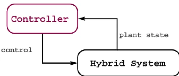
Hybrid System Controller
control u
plant state
Figure 2.1: Controlled hybrid system
issue plays important role in industry and it is challenging from the research point of view, one can hardly nd elaborated industrial applications in the literature [45].
Controller design for hybrid systems has become one of the hot topics in nowadays control theory, and there are tools based on advanced optimization methods [46] for designing controllers for dierent classes of hybrid systems. These tools are, however, not necessarily easy to use. A signal ow diagram of a controlled hybrid system can be seen in Fig. 2.1.
The traditional way of controlling hybrid process systems is to use model-predictive controllers.
Model predictive control (MPC) is a control paradigm of which underlying ideas originate from the 60's and later from the 70's as they became more widely used in petrochemical industry. There were quite a few variants of MPC which were not much dierent from algorithmic point of view, instead they used dierent process models. According to using state-space models dominated input-output models in the 90's the theory of MPC matured substantially.
MPC is an optimization based control law where, similar to most control methods, a perform- ance measureJ is minimized with respect to a certain prediction horizon. The measureJ is almost always based on quadratic forms or linear norms because using them simplies mathematical ana- lysis and leads to optimization problems that can be solved more eciently.
Nowadays a new approach has been emerged to control hybrid systems of special type based on multi-parametric programming optimization methods, which are collected in the Matlab MPT- toolbox (Multi-parametric Programming Toolbox).
2.3.1 Multi-parametric programs and their properties
The general form of multi-parametric programs is the following. Consider a nonlinear mathematical program which is dependent on a parameter vectorxand on certain constraints
Ex(k) +Lu(k)≤M (2.6)
fork∈Nand denote by constrained PWA system the restriction of system (2.5) that is subject to the constraints above:
x(k+ 1) = fP W A(x(k), u(k)) =Aix(k) +Biu(k) +fi y(k) = Cix(k) +Diu(k) +gi if
x(k) u(k)
∈P˜i, (2.7) where ∪iP˜i is the new polyhedral partition of the sets of states and inputs which is obtained by intersecting setsPi from Eq. (2.5) and the polyhedron dened by the constraints above:
In the framework of the dissertation the goal is to nd the optimal control input that minimizes a performance measure subject to the system dynamics and constrains on states or inputs by dening the performance weightL.
In the case of constrained innite time optimal control (CITOC) problem the performance measure is expressed as
J∞∗ (x(k)) = min
u∈U
∞
X
i=0
L(xk+i, uk+i) (2.8)
subject to the system model and constraints.
In the general case it is not possible to nd a closed form expression for the solution. Instead in the practice a horizon T is dened and J is approximated by using this nite horizon, like in
optimization problem obtain UT*
UT*HxL=:u0* , u1*…, uT*-1>
Hybrid System
plant state x output y apply u0*
Figure 2.2: MPC online optimization the case of constrained nite time optimal control (CFTOC) problem:
JT∗(x(k)) = min
u∈U LT(xk+T) +
T−1
X
i=0
L(xk+i, uk+i)
!
(2.9) subject to the system model and constraints. The solution of the CFTOC-problem is a nite input sequenceUT(x(k)).
Often this approach combined by applying the so-called receding horizon policy (RHC) which consists of the following steps (see in Fig. 2.2):
1. Measure the statex(k)at sampling instancek.
2. Solve the CFTOC-problem and get the input sequenceUT(x(k)). 3. Apply its rst element to the system as input.
4. Repeat from step 1.
The cost of a sequence of steps starting from a given initial state x(0) can be measured by computingJN∗ (x(0))as an LP or QP respectively for the cost objectives.
According to Eq. (2.9) designing a controller for this system is equivalent to solving a series of constrained nite-time optimal control (CFTOC) problem in closed-loop case:
JN∗ (x(0)) = min
u(0),...,u(N−1) kQfx(N)kl+
N−1
X
i=0
(kRu(i)kl+kQx(i)kl)
!
(2.10) subject to the constraints
x(k)∈X, ∀k∈ {1,2, . . . , N} (2.11)
x(N)∈Xf (2.12)
u(k)∈U, ∀k∈ {0,1, . . . , N−1} (2.13) Q=Q00, Qf =Q0f 0, R=R00 if l= 2 (2.14) rank(Q) =n, rank(R) =v if l∈ {1,∞}, (2.15) where Eq. (2.14) should be considered ifl = 2(quadratic cost), forl = 1(Manhattan-norm) and l=∞ (supremum norm) Eq. (2.15) holds. Eq. (2.12) is a user dened set-constraint on the nal stateXf which may be chosen such that stability of the closed-loop system is guaranteed (see [47]).
The matricesQ,Qf andRare weights on the states and inputs of appropriate dimension.
Denition 20. A setXfN ⊆Rn is called N-step feasible set if it contains those and only those initial states for which the CFTOC-problem (2.10) is feasible, i.e.,
XfN =
x(0)∈Rn| ∃(u(0), . . . , u(N−1))∈RN v, x(k)∈X, u(k−1)∈U, ∀k∈ {1, . . . , N} (2.16)
By substitutingx(k) =Akx(0) +Pk−1
j=0AjBu(k−1−j)to Eq. (2.10), it can be rewritten as JN∗ (x(0)) =x(0)0Y x(0) + minUN UN0 HUN +x(0)0F UN
s.t. GUN ≤W +Ex(0), (2.17)
where the column vectorUN = u00, . . . , u0N−10 and matricesH,F,Y,G,W andE are obtained from Eqs. (2.5) and (2.10) (which calculations are detailed in [48]).
Theorem 21. Consider the CFTOC problem. Then, the set of feasible states XfN is convex, the optimizer function is continuous and piecewise ane, i.e.,
UN∗ :XfN →RN v, UN∗ (x(0)) =Frx(0) +Gr ifx(0)∈ Rr, (2.18) where
Rr={x∈Rn|Hrx≤Kr}, r= 1,2, . . . , Z
and the optimal cost JN∗ : XfN → R is continuous, convex and piecewise quadratic if l = 2 or piecewise linear if l= 1orl=∞.
Proof. See [48].
According to this theorem the feasible state space XfN is partitioned intoZ number of poly- topic regions, i.e., XfN = { Rr}Zr=1. With suciently large horizons or appropriate terminal set constraints the closed-loop system is guaranteed to be stabilizing for receding horizon control.
The following theorem ([47]) provides the main stability result that ensures the closed loop stability of RHC.
Theorem 22. Suppose that
1. The sets X andU contain the origin and Xf is closed, 2. Xf is control invariant, i.e.,Xf ⊆X,
3. ∀x∈Xf : minu∈U, Ax+Bu∈XfkP(Ax+Bu)kl− kP xkl+kQxkl+kRukl≤0 4. kP xkl≤β(|x|), whereβ is a function of classK.
Then the state of the closed-loop system converges to the origin and also the origin of the closed-loop system is asymptotically stable with the DOA beingXf.
Proof. See [46].
To design a controller using MPT one has to have the model description equations in DT- domain so one has to discretize the model if it is necessary. Choosing the appropriate sampling time will be discussed later in subsection 5.2.1.
Apparently all multi-parametric programming methods are suering from the problem of di- mensionality. As the prediction horizonN increases, the number of partitionsR in Theorem 21 grows exponentially.
2.4 Nonlinear dynamic model of pressurized water reactor systems
Nuclear power plants represent one of the most important and environmentally friendly way of obtaining energy, and they are widely used worldwide. Because of economical and safety reasons, these plants apply advanced technology and use sophisticated data monitoring and control meth- ods, but possess highly nonlinear complex dynamics. Nuclear power plants are among the most elaborated hybrid systems, i.e., systems with both continuous and discrete variables, ever designed so it is of vital importance to be able to determine the stability region around their operating point to make sure that they operate within a stable region.
This dissertation presents dierent versions of stability analyses, the DOA analysis of various forms of the primary circuit system which is in current use in the Paks Nuclear Power Plant (Paks NPP) located in Hungary. The Paks NPP was founded in 1976 and started its operation in 1981.
The plant operates four VVER-440/213 type reactor units with a total nominal (electrical) power of 1860 MWs that are of pressurized water reactor (PWR) type. About 40 percent of the electrical energy generated in Hungary is produced here. Considering the load factors, the Paks units belong to the leading ones in the world and have been among the top twenty-ve units for years.
A low dimensional nonlinear dynamic model with the most important controllers for the primary circuit in a VVER-type nuclear power plant has been developed based on rst engineering principles (discussed in [1]) that is able to capture the most important dynamics of the system in its normal operating modes (see [49]).
The model developed in [49] serves as a basis for the dierent versions that are used in this thesis. First a third-order model is derived for the controlled system; thereafter this model is simplied in order to make it appropriate for the further stability analyses.
2.4.1 Stability analysis of nuclear system models
Dynamic modelling and stability analysis of nuclear reactors are in the focus of research nowadays.
In [50] a simple mathematical model has been developed to describe the dynamics of the nuclear- coupled thermal-hydraulics in a boiling water reactor (BWR) core incorporating the essential features of neutron kinetics and thermal-hydraulics. The stability boundary was determined and plotted in the inlet-subcooling-number/external-reactivity operating parameter plane. The ana- lysis of eigenvalues of the Jacobian matrix was shown to be consistent with direct stability analysis showing that a Hopf-bifurcation occurs at the stability boundaries. In [51] the spectrum of Lya- punov exponents (calculated by using of the Jacobian matrix [52]) was considered as a dynamical diagnosis tool for instability of a nuclear reactor model. It was found that in supercritical state a Lyapunov exponent is positive which implies that the reactor governed by neutron diusion phenomena (according to [53]) is chaotic. In [54] a theoretical model describing the coupling of neutronics, thermohydraulics and uidization in a uidized bed nuclear reactor and its stability analysis is presented by linearising and perturbing by simulations the system around its equilibrium points. In [55] asymptotic stability regions of nonlinear reactor models are estimated using iterative expansion both a specic Lyapunov-function and any positive denite function. The shown meth- ods do not require solving the model equations instead they solve an algebraic equation which the stability domain satises. Stability investigations may involve mechanical-uid-dynamical features like ow excursions or density wave oscillations (see [56]).
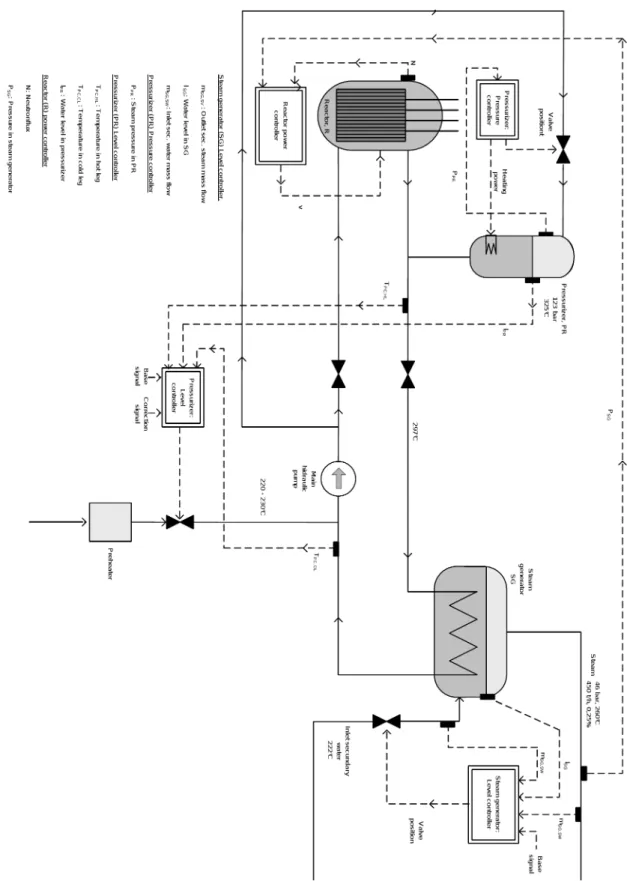
2.4.2 Modelling assumptions
Figure 2.3 shows the dierent operating units of the primary circuit and their connections which are taken into account in the simplied model. The controllers are denoted by double rectangles, their input and output signals are shown by dashed lines and the sensors that provide on-line measurements are also indicated in the gure by small full rectangles.
The steady-state values of the system variables in the normal 100 % power operating point are also indicated in Figure 2.3.
From the viewpoint of their dynamics and the type of their dependence on other operating units, the units of the simplied dynamic model are classied into three groups:
• The reactor which has a fast dynamics compared to the other operating units while its dynamics depends directly only on the temperature of the water in the primary circuit that is neglected.
• The water in the primary circuit and the steam generator which are the units that transport the energy generated by the reactor to the secondary circuit.
• The pressurizer that supplies a constant regulated pressure for the primary circuit.
For convenience, unique identiers are used for the operating units in the subscript of their related variables and parameters, as well as in all related modelling items, such as assumptions, that are listed below:
R reactor
PC primary circuit PR pressurizer SG steam generator
The overall modelling assumptions specify the considered operating units and their general prop- erties which are:
• The set of operating units considered in the simple dynamic model includes the water in the tubes of the primary circuit (PC) and the pressurizer (PR).
• The dynamic model of the operating units is derived from simplied energy balances con- structed for a single balance volume that corresponds to the individual unit.
• The only considered controller in the simplied model is the pressure controller. All the other controllers (including the level controller in the pressurizer, and the controller of the turbines, main circulating pumps and other compressors and valves in the system) are assumed to be ideal, that is, they keep their reference values ideally, without any dynamics or delays.
• The mass in the primary circuit (MP C) is constant.
• The reactor is a system with concentrated parameters.
• The so-called one-group diusion-theoretical approach was considered.
• Only the late neutron emitting nuclei group was taken into account.
In order to obtain a low dimensional dynamic model, the simplest possible set of operating units is considered in their simplest functional form. Part of the primary circuit with clear functionality is considered as an operating unit. An operating unit may contain several physical units (pipes, containers, valves, etc.) but it is then regarded as a primary balance volume over which conservation balances can be constructed.
2.4.3 Conservation balances
The model-equations presented in this section are derived from the ones developed in [49] with simplications that made possible the further analyses and they keep the hybrid behaviour, i.e., the temperature of the water in the pressurizer depends on the ow direction to/from the pressurizer.
The core of the model equations contains dierential or dynamical equations that originate from conservation balances.
The rst dynamics describes the temperature of the water in the primary circuitTP C: dTP C
dt = WR(v)−6KSGT (TP C−TSG)−WP Closs
MP CcpP C , (2.19)
whereWR(v)is the power of the reactor given by Eq. (2.23) later,KSGT is the PC-SG heat transfer coecient,WP Closs is the SG heat loss, MP C is the PC water mass,cpP C is the PC specic heat of water (on 282◦C),TSG∗ is the nominal SG temperature andvis the position of the rod in expressed incm's.
The second one describes the dynamics of the temperature of the water in the pressurizerTP R: dTP R
dt = WP Rheat−WP Rloss−cpP RmP R(v)TP R+h(v)
MP RcpP R , (2.20)
Figure 2.3: Process ow-sheet with the operating units of the simplied model
where WP Rheat is the heating power of the pressurizer,WP Rloss is the PR heat loss, cpP R is the water specic heat (on 282◦C) in the pressurizer andh(v)describes the hybrid behaviour depending on the in/out mass ow from the primary circuitmP R(v)(see Eq. (2.29) later).
The third one describes the dynamics of the temperature of the water in the steam generator TSG:
dTSG
dt = KSGT (TP C−TSG)−cpSG,vmSGTSG−WSGloss
MSGcpSG,l , (2.21)
whereMSG is the mass of water in the steam generator,cpSG,lis the specic heat of the water and cpSG,vis the specic heat of the vapour in the secondary circuit,mSGis the constant mass ow rate of the water and steam in the secondary circuit andWSGlossis the heat loss of the steam generator.
The last dynamic equation of the reactor follows from the conservation balances for the neutron- uxN:
dN
dt =S+βN
Λ p1v2+p2v+p3
, (2.22)
whereS is the ux of the constant neutron source,β is the late neutron ratio,Λis the generation time,p1,2,3are the rod reactivity-coecients andv is the rod's position.
2.4.4 Algebraic constitutive equations
The dynamic conservation energy equations of the controlled primary circuit model form the state equations that are complemented with substitutable algebraic equations.
The reactor powerWR is proportional to the neutron uxN
WR(v) =cψN(v) (2.23)
wherecψ is a given constant.
Supposing that the dynamics of the neutron ux is much faster than any other of the examined phenomena we can use the assumption dNdt = 0which yields
N(v) = SΛ
β(p1v2+p2v+p3). (2.24) The PR liquid mass MP R is computed by assuming that the density of the liquid is a known quadratic function of the temperature, i.e.,
ρP C=cϕ0+cϕ1T˜P C+cϕ2T˜P C2 (2.25) and can be described as
MP R=MP C−VP C0 ρP C, (2.26)
whereMP C is the mass of the PC water,VP C0 is a nominal volume of the primary circuit,T˜P C is the PC temperature measured in Celsius, andcϕ0,cϕ1 andcϕ2 are constants.
The PR heating powerWP Rheatis controlled by a proportional (P) controller as a function of the deviation of the temperatureTP R (that is proportional to the pressure) in the pressurizer from its reference valueTP R∗
WP Rheat=WP Rloss−KP R(TP R−TP R∗ ), (2.27) whereKP R is a feedback gain of the pressure controller.
The in/out mass ow mP R(WR) from the primary circuit is computed as the time-derivative ofMP R in Eq. (2.26)
mP R(v) =−VP C0 (cϕ1+ 2TP Ccϕ2)dTP C
dt (2.28)
The hybrid behaviour The hybrid behaviour is generated by the fact that the temperature of the in/out mass ow (Eq. (2.20)) to/from the pressurizer mP R(v) is dierent depending on the ow direction as follows:
h(v) =
(cpP CmP R(v)TP Chotleg mP R(v)>0
cpP RmP R(v)TP R mP R(v)≤0 (2.29)