The final publication is available at
https://link.springer.com/article/10.1007%2Fs10936-018-9558-7 Csilla Rákosi
MTA-DE-SZTE Research Group for Theoretical Linguistics Dealing with the conflicting results of psycholinguistic experiments:
How to resolve them with the help of statistical meta-analysis
Abstract
This paper proposes the use of the tools of statistical meta-analysis as a method of conflict resolution with respect to experiments in cognitive linguistics. With the help of statistical meta- analysis, the effect size of similar experiments can be compared, a well-founded and robust synthesis of the experimental data can be achieved, and possible causes of any divergence(s) in the outcomes can be revealed. This application of statistical meta-analysis offers a novel method of how diverging evidence can be dealt with. The workability of this idea is exemplified by a case study dealing with a series of experiments conducted as non-exact replications of Thibodeau & Boroditsky (2011).
Keywords: experiments on metaphor processing; replication of experiments; statistical meta- analysis; inconsistency resolution; diverging evidence
1. Introduction
Experiments often produce diverging evidence in cognitive linguistics, because (non-exact) replications conducted by adherents of rival theories typically lead to conflicting results. There is, however, no generally accepted methodology of conflict resolution which could be applied in such cases. Rákosi (2017a,b) presented a novel metatheoretical framework that might make it possible to grasp the relationship between original experiments and their non-exact replications, and evaluate the effectiveness of the problem solving process. The central concept of this framework is the notion of ‘experimental complex’. Experimental complexes consist of chains of closely related experiments which are modified (refined, improved) versions of an original experiment. The proposed metatheoretical model shows that the relationship among these experiments is determined by the operation of recurrent re-evaluation: newer, more refined and revised versions replace earlier ones. From this finding a possible method of conflict resolution arises. Namely, one should aim at detecting starting points which might lead to the elaboration of a novel version of the original experiment which can be, at least temporarily, regarded as acceptable (valid and reliable) by continuing the re-evaluation process.
Nevertheless, there is another possible route which can be taken in order to summarise the outcome of a series of experiments and find guidelines for the elaboration of new, more sophisticated experiments: statistical meta-analysis. Instead of reconstructing the re-evaluation process and elaborating proposals for a more refined version of the experiment at issue on the basis of the outcome of the reconstruction, meta-analysis attempts to accumulate all available pieces of information so that the shortcomings of individual experiments can be counterbalanced, and more robust results can be obtained. As Geoff Cumming puts it,
“Meta-analytic thinking is estimation thinking that considers any result in the context of past and potential future results on the same question. It focuses on the cumulation of evidence over studies.” (Cumming, 2012: 9)
Statistical meta-analysis is the application of statistical thinking and of statistical tools at a meta-level. The objects of this meta-level analysis are the results of a series of experiments as data points. Its aim is to estimate the strength of the relationship between two (or more) variables, that is, it works with effect sizes, first at the level of the individual experiments and then at the level of their synthesis. There are several types of effect size (Pearson’s correlation coefficient, Cohen’s d, odds ratio, raw difference of means, risk ratio, Cramér’s V, etc.), which can be converted into each other.
According to Borenstein et al. (2009: 297ff.), this method is preferable to the customary approach of hypothesis testing. First, the p-value only tells us whether it is highly improbable that there is no effect, while focusing on the effect sizes is considerably more instructive because it also provides information about the magnitude of the effect. That is, a higher effect size indicates a stronger relationship between the variables. To put it differently, test statistics tells us only whether there is an effect of one variable on another which could be not merely due to chance – irrespective of the circumstance that this effect is considerable or negligible.1 In contrast, effect size values give us accurate information about the strength of the relationship between two variables. Moreover, if we calculate confidence intervals for them, then they also reveal whether the result is statistically significant. In this way, we may obtain information about
– the magnitude of the effect (distance from the null-value);
1 If the sample size is large enough, even a very small effect can be significant.
– the direction of the effect (positive vs. negative, showing an effect in the predicted or the opposite direction);
– the precision of the effect estimate (width of the confidence interval).
Second, the use of test statistics often leads to dichotomous thinking (cf. Cumming 2012: 8f.) and vote counting: x significant vs. y non-significant results – but it is not clear what they mean together. The application of effect sizes, however, makes it possible to compare and synthesize the outcome of a set of similar experiments. Thus, for example,
– there may be a considerable overlap among their confidence intervals (or one of them may completely contain the other one), indicating a harmony among the results of the different experiments;
– the confidence intervals may be totally distinct, pointing to a case of heterogeneity;
– between these two extremes, there may be a small overlap among the confidence intervals, suggesting the compatibility of the results;
– even if one of the confidence intervals includes the null value (indicating a non-significant result) while the other confidence interval is above the null value, the two experiments’
results may be compatible or even in harmony.
Therefore, statistical meta-analysis seems to be a possible tool of conflict resolution related to non-exact replications. It allows us to calculate a summary effect size by taking into consideration the effect size of the individual experiments, their precision (confidence intervals) and size (number of participants). To put it differently, statistical meta-analysis combines the effect sizes of similar experiments in such a way that larger and more precise experiments are assigned greater weight.
Against this background, this paper raises the following problem:
(P) How can conflicting results of psycholinguistic experiments be resolved with the help of statistical meta-analysis?
This paper does not intend to solve this question in general but rather to show the workability of this idea with the help of an instructive case study. Between 2011 and 2015, Thibodeau &
Boroditsky, and Steen and his colleagues conducted a series of experiments intended to test the hypothesis that “exposure to even a single metaphor can induce substantial differences in opinion about how to solve social problems” (Thibodeau & Boroditsky, 2011: 1). The two series of replications by the two camps repeatedly came to opposite conclusions. While Thibodeau and Boroditsky concluded, for example, that
“We find that exposure to even a single metaphor can induce substantial differences in opinion about how to solve social problems: differences that are larger, for example, than pre-existing differences in opinion between Democrats and Republicans.” (Thibodeau &
Boroditsky 2011: 1), the other camp stated that
“We do not find a metaphorical framing effect.” (Steen et al. 2014: 1)
“Overall, our data show limited support for the hypothesis that extended metaphors influence people’s opinions.” (Reijnierse et al. 2015: 258)
Nonetheless, there are some important caveats. Statistical meta-analyses and systematic reviews have a very strict standard protocol called the ‘PRISMA 2009 checklist’. We will follow its stipulations only loosely, for four reasons. First, this paper is not a systematic review
but applies the tools of statistical meta-analysis in a novel way.2 This means, above all, that it does not intend to cover all experiments dealing with the same or a similar research question as published so far but intends to investigate whether and how meta-analytic tools can be applied to conflict resolution with the help of an instructive case study.3 That is, the focus of the paper is not on the object-scientific question of whether metaphors influence thinking but the meta-scientific question of how to deal with inconsistencies between closely related experiments. From this point of view, the extension of the number of the experiments included is not decisive. Second, since meta-analysis is applied to a limited number of experiments, there are unavoidably some deviations from the customary practice. Third, statistical meta- analysis does not belong to mainstream methods applied in cognitive linguistics. Therefore, the paper does not divide into a classic “methods – data – results – conclusions” structure but a brief explanation of the basic concepts of meta-analysis, and their application to the experiments of the case study is presented step-by-step. Fourth, the researchers conducting the experiments made their data sets public. Hence, there is room for deeper analyses as well as re-analyses.
The structure of the paper is as follows. Section 2 explains the procedure of selecting the experiments included in the meta-analysis. Section 3 describes the methods applied in the choice of the effect size index and the data collection process and shows how effect sizes can be calculated at the level of the individual experiments if we focus on the participants’ top choices. Section 4 deals with the combination of the experiments’ effect sizes, that is, the calculation of the summary effect size, the methods used to check their consistency, as well as methods for revealing possible publication bias, and then presents the results. Section 5 presents alternative analyses: an analysis which takes into consideration the whole range of the measures and an analysis comparing the effect of the metaphorical frames on the measures separately. Section 6 summarises the main findings, draws conclusions and discusses the limitations of the results.
2. The selection of experiments included in the meta-analysis
The first step of the meta-analysis is the selection of the experiments. The decisive point is that in order to be combinable all experiments have to test the same research hypothesis, or their research hypotheses have to share a common core. The reason for this lies in the circumstance that meta-analysis produces a statistical synthesis of the effect sizes of the individual experiments. This means that all experiments should provide information about the relationship between two variables, so that the strength of this relationship is determinable in each case.
The experimental complex evolving from Thibodeau & Boroditsky (2011) comprises a
2 “[…]‘research synthesis’ and ‘systematic review’ are terms used for a review that focuses on integrating research evidence from a number of studies. Such reviews usually employ the quantitative techniques of meta-analysis to carry out the integration.” (Cumming 2012: 255; emphasis added)
“A key element in most systematic reviews is the statistical synthesis of the data, or the meta-analysis. Unlike the narrative review, where reviewers implicitly assign some level of importance to each study, in meta-analysis the weights assigned to each study are based on mathematical criteria that are specified in advance. While the reviewers and readers may still differ on the substantive meaning of the results (as they might for a primary study), the statistical analysis provides a transparent, objective, and replicable framework for this discussion.”
(Borenstein et al., 2009: xxiii; emphasis added)
3 Since the selection of relevant studies always and unavoidably leaves room for subjective factors, nothing precludes a restricted use of the tools of meta-analysis to a smaller but well-defined set of experiments:
“For systematic reviews, a clear set of rules is used for studies, and then to determine which studies will be included in or excluded from the analysis. Since there is an element of subjectivity in setting these criteria, as well as in the conclusions drawn from the meta-analysis, we cannot say that the systematic review is entirely objective. However, because all of the decisions are specified clearly, the mechanisms are transparent.”
(Borenstein et al., 2009: xxiii; emphasis added)
series of experiments investigating the effect of metaphorical framing on readers’ preference for frame-consistent/inconsistent political measures. The following short description of the experiments should be sufficient to show that the majority of them are similar enough and that it is possible to apply the tools of meta-analysis to their results.
Thibodeau & Boroditsky (2011), Experiment 1: Participants were presented with one version of the following passage:
“Crime is a {wild beast preying on/virus infecting} the city of Addison. The crime rate in the once peaceful city has steadily increased over the past three years. In fact, these days it seems that crime is {lurking in/plaguing} every neighborhood. In 2004, 46,177 crimes were reported compared to more than 55,000 reported in 2007. The rise in violent crime is particularly alarming. In 2004, there were 330 murders in the city, in 2007, there were over 500.”
Then, they had to answer the open question of what, in their opinion, Addison needs to do to reduce crime. The answers were coded into two categories on the basis of the results of a previous norming study: 1) diagnose/treat/inoculate (that is, they suggested introducing social reforms or revealing the causes of the problems) and 2) capture/enforce/punish (that is, they proposed the use of the police force or the strengthening of the criminal justice system).
Thibodeau & Boroditsky (2011), Experiment 2: In this experiment, the passage to be read, besides a metaphor belonging to one of the two metaphorical frames, also included further ambiguous metaphorical expressions which could be interpreted in both metaphorical frames.
The task was to suggest a measure for solving the crime problem, and explain the role of the police officers in order to disambiguate the answers.
Thibodeau & Boroditsky (2011), Experiment 4: The only change in comparison to Experiment 2 pertains to the type and focus of the task: instead of the application of an open question about the most important/urgent measure, participants had to choose one issue for further investigation from a 4-member list:
1. Increase street patrols that look for criminals. (coded as ‘street patrols’) 2. Increase prison sentences for convicted offenders. (‘prison’)
3. Reform education practices and create after school programs. (‘education’) 4. Expand economic welfare programs and create jobs. (‘economy’)
Thibodeau & Boroditsky (2013), Experiment 2: The wording of the task was modified substantially against Experiment 4 of Thibodeau & Boroditsky (2011) in order to touch upon participants’ attitudes towards crime reducing measures directly. Namely, it consisted of selecting the most effective crime-reducing measure from a range of 4.
Thibodeau & Boroditsky (2013), Experiment 3: The only change made to Experiment 2 was the extension of the selection of measures with the ‘neighbourhood watches’ option (“Develop neighborhood watch programs and do more community outreach.”).
Thibodeau & Boroditsky (2013), Experiment 4: There was only a slight difference between this experiment and its predecessor: the technique the participants used to evaluate the 5 measures was modified. That is, their task was to rank 5 crime-reducing measures according to their effectiveness. Nonetheless, only the top choice was used for the creation of the experimental data by the authors.
Steen et al. (2014), Experiment 1: The authors extended the stimulus material with a no- metaphor version, in order to provide a neutral point of reference, and a version without further metaphorical expressions (a ‘without support’ version). Here, too, participants had to rank the 5 crime-reducing measures according to their effectiveness before and after reading the passage about crime.
Steen et al. (2014), Experiment 2: Only the language was changed from Experiment 1 (English instead of Dutch).
Steen et al. (2014), Experiments 3-4: The idea of a pre-reading evaluation of the measures was rejected. Thus, the task for the participants consisted of ranking the five crime-reducing measures according to their effectiveness only after reading the passage about crime. The only difference between Experiments 3 and 4 was the number of participants: the latter used a higher number of participants so as to have the power to detect small effects, as well.
Thibodeau & Boroditsky (2015), Experiment 1: The only change to Experiment 3 in Thibodeau & Boroditsky (2013) was the application of three control experiments in order to improve the stimulus material’s validity.
Thibodeau & Boroditsky (2015), Experiment 2: The novelty of this member of the experimental complex is that it reduces the impact of the binary coding of the five measures in such a way that only the two most prototypical choices were offered for participants to decide between.
Reijnierse et al. (2015), Experiment 1: This experiment made use of 1 story in 2 versions (no-metaphor/‘virus’ frame). The metaphorical content was varied so that the passage to be read by participants contained 0, 1, 2, 3, or 4 metaphorical expressions. The task consisted of evaluating 4+4 crime-reducing measures according to their effectiveness on a 7-point Likert- scale. Then, the average of the enforcement-oriented vs. reform-oriented values were compared.
Reijnierse et al. (2015), Experiment 2: Identical to Experiment 1, except that there was a
‘beast’ frame instead of a ‘virus’ frame.
Christmann & Göhring (2016): This was an attempt at an exact replication of Thibodeau &
Boroditsky (2011), Experiment 1 in German.
In contrast, the following three experiments had to be excluded from the meta-analysis:
Thibodeau & Boroditsky (2011), Experiment 3: The stimulus material did not contain metaphors. Instead, participants had to provide synonyms for the words ‘virus’ or ‘beast’, suggest a measure for crime reduction, and explain the role of police officers. Since there were no metaphors in the passage to be read, this experiment will be excluded from the meta- analysis.
Thibodeau & Boroditsky (2011), Experiment 5: Thibodeau & Boroditsky (2011), Experiment 5: In contrast to Experiment 4, the metaphor belonging to one of the two metaphorical frames was presented at the end of the passage. Presentation of the target metaphor at the end of the passage leads to a situation which is substantially different from the previous experiments.
Thibodeau & Boroditsky (2013), Experiment 1 was a control experiment.
3. The choice and calculation of the effect size of the experiments 3.1. The data structure of the experiments
The brief characterization of the experiments in the previous section and a closer look at the data handling techniques of the authors reveal a highly important issue: namely, both the tasks which the participants had to perform and the methods for creating experimental data from the raw (perceptual) data were different in the experiments at issue.
Thibodeau & Boroditsky (2011), Experiments 1, 2 and 4
Experiment 1 utilized an open question task. Participants’ answers were first coded separately by the authors into the two categories ‘social reform’ vs. ‘enforcement’, and then rendered as either purely social-type (1-0), purely enforcement-type (0-1) or mixed (0.5-0.5). In Experiment 2, this procedure was also applied to the question about the role of the police, and the two answers were averaged. In Experiment 4, participants had to choose one measure.
Thibodeau and Boroditsky coded the answers as either social reform-oriented or enforcement- oriented.
Thibodeau & Boroditsky (2013), Experiments 2-4
The data sets pertaining to Experiments 3 and 4 have been made accessible by the authors at https://osf.io/r8mac/. These data sets do not include information about the whole ranking of the measures but only participants’ first choices. In the evaluation of the data, the authors also included participants’ second choices, and examined their orientedness and coherence with the metaphorical frame.
Steen et al. (2014), Experiments 1-4
The data sets can be downloaded from https://osf.io/ujv2f/ as SPSS data files. Both the post- reading and pre-reading responses of participants were captured, and there was also a ‘with metaphorical support’ versus ‘without support’ version. The first two choices were taken into consideration by the researchers. The answers were coded with the help of the following 3- point scale: +2 (two enforcement-oriented choices in the first two places) / +1 (one enforcement-oriented and one social reform oriented choice / 0 (two social reform-oriented choices). The results of participants with a shorter reading time than 5s or longer than 60s, and those under 18 years of age were excluded. Residency different from the Netherlands/US and native language different from Dutch/English were not allowed, either.
Thibodeau & Boroditsky (2015)
The range of the experimental data and the methods of their treatment were almost identical with those used in the case of Experiments 2-4 in Thibodeau & Boroditsky (2013).
Reijnierse et al. (2015), Experiments 1-2
The data have been made public on the following Open Science Framework site:
https://osf.io/63ym9/. The authors processed the data in such a way that they examined the effect of the number of metaphorical expressions on the perceived efficiency ratings of the two types of measures with the help of a one-way independent ANOVA, separately with both frames.
Christmann & Göhring (2016): Similarly to Experiment 1 of Thibodeau & Boroditsky (2011), an open question task was applied. The coding system has been, however, modified.
Since the number of answers which could not be assigned to the category ‘social reform’ or
‘enforcement’ was relatively high, the authors excluded them from their analyses. Table 1 on
page 4 contains the response frequencies. The authors, however, made all the answer sheets available at the Open Science Framework site https://osf.io/m7a5u/. I used this data source, and revised the authors’ decisions on some occasions.
3.2. The choice of the effect size indicator
In order to reduce the impact of the diversity of methods applied by the researchers, the data handling techniques have to be standardized. The most straightforward possibility is to analyse the impact of the frames (beast vs. virus) on the orientedness (social reform vs. enforcement) of the top choices. The question is, of course, how this can be achieved.
The simplest way to calculate the effect of the metaphorical frames on the choice of the measures consists of comparing the odds of choosing a social type response against choosing an enforcement type response in the first place in the virus condition and the odds of choosing a social type response against choosing an enforcement type response in the first place in the beast condition – i.e. computing the odds ratio:4
OR =
odds of choosing a social type response against choosing an enforcement type response in the
first place in the virus condition =
odds of choosing a social type response against choosing an enforcement type response in the first place in the beast condition
=
number of participants choosing a social type response in the first place in the virus condition / number of participants choosing an enforcement-type response in the first place in the virus condition
number of participants choosing a social type response in the first place in the beast condition / number of participants choosing an enforcement-type response in the first place in the beast condition
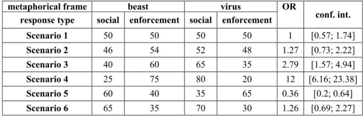
In order to illustrate how different OR values can be interpreted, let us experiment with some possible scenarios:
metaphorical frame beast virus OR
conf. int.
response type social enforcement social enforcement
Scenario 1 50 50 50 50 1 [0.57; 1.74]
Scenario 2 46 54 52 48 1.27 [0.73; 2.22]
Scenario 3 40 60 65 35 2.79 [1.57; 4.94]
Scenario 4 25 75 80 20 12 [6.16; 23.38]
Scenario 5 60 40 35 65 0.36 [0.2; 0.64]
Scenario 6 65 35 70 30 1.26 [0.69; 2.27]
Table 1: OR value calculations
In Scenario 1, we see a perfect tie between social reform- and enforcement-oriented first choices. This yields an odds ratio of 1. That is, if OR is 1, then we can conclude that the metaphorical frame does not affect the choice of the responses. In Scenario 2, with both frames, the frame-consistent answers were slightly preferred by participants. This yields an OR somewhat greater than 1. In Scenario 3, the frame-consistent choices approach a two-thirds majority – and the OR approaches a value of 3. If more than 75% of participants give a frame-
4 There are several effect size indicators which can be calculated with dichotomous variables. Among these, the odds ratio is the most versatile (but not intuitively interpretable).
consistent answer, then the OR rises to 12. Scenario 5 shows what happens if participants chose frame-inconsistent responses: the OR is between 0 and 1. Finally, in Scenario 6, in both frames it is the social reform-type choices that are in the majority. Since the proportion of the frame- consistent answers is slightly higher in the virus frame than that of the frame-inconsistent responses in the beast frame, we obtain an OR slightly higher than 1.
It is vital to take into consideration the precision of these estimates, too. To this end, we can calculate the 95% confidence intervals of the OR values. This shows a range which – in 95% of cases – encompasses the odds of choosing a social type response against an enforcement type response in the virus condition compared to the beast condition. For example, the confidence interval in Scenario 5 is narrow. This indicates that the precision of the estimate is high. In this case, the confidence interval does not overlap the value 1. Therefore, we can conclude that participants who obtained the crime-as-virus metaphorical framing preferred social reform-type answers significantly less frequently than those who read the crime-as-beast framing.5 In contrast, in Scenarios 3 and 4, participants gave frame-consistent answers significantly more often, since the whole confidence interval is above the value 1 – although the precision of these estimates is lower, as the width of the confidence interval shows.
Scenarios 1, 2 and 6, however, did not produce significant results, because their confidence intervals include the value 1.
As a next step, we need data from which the odds ratio can be calculated for each experiment. In some cases, this was an easy task, in other cases, further data had to be collected from the authors and/or some work was needed to extract the relevant information from the data sets available.
3.3. Methods of data collection
With the help of the CMA software, effect sizes can be computed from about 100 options, i.e., more than 100 summary data types, but there are also several online effect size calculators such as this one: https://www.psychometrica.de/effect_size.html. Since the data sheets made available by the researchers on a special Open Science Framework site or via email make it possible to collect information about the events and sample size in each group, it is better (i.e., will result in more precise effect size values) to make use of these data (and apply the formula presented in the previous section) than, for example, the Chi-squared and the total sample size, as published in the research papers. This decision is motivated by the finding that if there are several possibilities, then the method which is closer to the raw data should be preferred.
Reliance on the summary data presented in the experimental reports is not a compulsory step of meta-analysis but often a necessity, because we do not usually have access to the data sets.
This means that from this set of experiments, data with the following structure should be extracted:
– the number of participants choosing a social reform type measure in the beast condition;
– the number of participants choosing an enforcement type measure in the beast condition;
– the number of participants choosing a social reform type measure in the virus condition;
– the number of participants choosing an enforcement type measure in the virus condition.
In most cases, these data could not be found in the research report but could be produced from the information in the data sheets. For details of this process, as well as the response frequencies in the individual experiments, see the following Open Science Framework page:
5 “There is a necessary correspondence between the p-value and the confidence interval, such that the p-value will fall under 0.05 if and only if the 95% confidence interval does not include the null value [with the odds ratio, this is 1]. Therefore, by scanning the confidence intervals we can easily identify the statistically significant studies.”
(Borenstein et al., 2009: 5)
https://osf.io/8xjbs/?view_only=b1013469554e409684b258c81666f105.
3.4. The effect size of the individual experiments
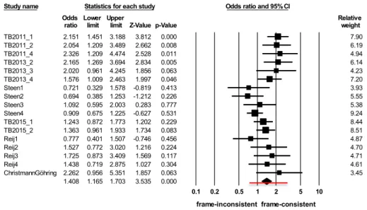
Figure 1 shows the individual effect sizes, their confidence intervals, Z-values, p-values, and weights.
Figure 1: Effect sizes of the experiments and the summary effect size in the first analysis (top choices of participants)
The odds ratios of the individual experiments ranged from 0.694 (Steen et al., 2004, Experiment 2) to 2.326 (Thibodeau & Boroditsky 2011, Experiment 4). An odds ratio greater than 1 means that participants preferred frame-consistent answers, while an odds ratio below 1 means the opposite. In 13 of the 17 cases, the odds ratio was higher than 1. There seem to be subgroups regarding the effect size values. Experiments in Thibodeau & Boroditsky (2011, 2013), except for Experiment 4 of their 2013 series of experiments, as well as the replication by Christmann & Göhring indicate an effect size slightly greater than 2. Thibodeau and Boroditsky’s 2015 paper shows effect sizes somewhat above 1. Experiments 1 and 2 in Steen et al. (2014) and the 1-metaphor condition in Reijnierse (2015) produced effect sizes clearly below 1. Experiments 3-4 in Steen (2014) are very close to 1, while the remaining experiments conducted by these authors indicate an effect size around the 1.5-mark. This means, in sum, that the experiments show a weak or no effect of the metaphorical frame.
There were only 5 experiments for which the confidence interval did not include the value 1. These all are completely above the 1-mark line, and represent a significant result for the research hypothesis. In contrast, there was no experiment which would provide a significant result against Thibodeau & Boroditsky’s research hypothesis. The lowest point of the confidence intervals was 0.329, while the highest was 5.351.
Experiment 4 of Steen et al. (2014) provides the most precise estimation of the effect size with a quite narrow confidence interval of [0.675, 1.225], while the replication by Christmann
& Göhring (2016) is the least precise: its confidence interval of [0.956, 5.351] is noticeably wide.
From these results it would be premature to conclude that the majority decides and the experiments together yield a statistically insignificant, weak support for Thibodeau and Boroditsky’s research hypothesis. The aim of meta-analysis is, as we have already said in Section 1, not to count votes but to calculate an estimate of the effect size on the basis of all the information inherent in the data from the experiments synthesized. There are several
Study name Statistics for each study Odds ratio and 95% CI
Odds Lower Upper Relative Relative
ratio limit limit Z-Value p-Value weight weight
TB2011_1 2.151 1.451 3.188 3.812 0.000 7.90
TB2011_2 2.054 1.209 3.489 2.662 0.008 6.19
TB2011_4 2.326 1.209 4.474 2.528 0.011 4.94
TB2013_2 2.165 1.269 3.694 2.834 0.005 6.14
TB2013_3 2.020 0.961 4.245 1.856 0.063 4.23
TB2013_4 1.576 1.009 2.463 1.997 0.046 7.20
Steen1 0.721 0.329 1.578 -0.819 0.413 3.93
Steen2 0.694 0.385 1.253 -1.212 0.226 5.55
Steen3 1.092 0.595 2.003 0.283 0.777 5.38
Steen4 0.909 0.675 1.225 -0.627 0.531 9.24
TB2015_1 1.243 0.872 1.773 1.202 0.229 8.44
TB2015_2 1.363 0.961 1.933 1.734 0.083 8.51
Reij1 0.777 0.401 1.507 -0.746 0.456 4.87
Reij2 1.527 0.772 3.020 1.216 0.224 4.70
Reij3 1.725 0.873 3.409 1.569 0.117 4.71
Reij4 1.438 0.719 2.875 1.027 0.304 4.61
ChristmannGöhring 2.262 0.956 5.351 1.857 0.063 3.45
1.408 1.165 1.703 3.535 0.000
0.1 0.2 0.5 1 2 5 10
frame-inconsistent frame-consistent Meta Analysis
methods for achieving this aim. The next section presents them and shows how the chosen method can be applied in this case.
4. Synthesis of the effect sizes
4.1. Methods for calculating the summary effect size
Having established the effect sizes of the experiments, the next step consists of estimating the summary effect size. This step was carried out with the help of the CMA software. There are basically two methods to combine the effect sizes of individual experiments: the fixed-effect model and the random-effect model. Following Borenstein et al.’s (2009: Part 3) characterisation, the two methods can be described as follows.
The fixed-effect model should be applied if the experiments to be combined made use of the same design, their participants share all relevant characteristics which might influence their performance, they were performed at (almost) the same time by the same researchers in the same laboratory, etc. If all circumstances are practically identical in each case, then we can suppose that the experiments have the same true (underlying) effect size, and any difference between the values in the individual studies is due solely to sampling error. Thus, fixed-effect models offer an estimation of the common (underlying, true) effect size. Random-effect models, in contrast, can be applied if, despite their important similarities, there are also substantial differences among the experiments. In fact, in the great majority of cases, we have to assume that the experiments differ from each other regarding their underlying (true) effect size. Our task is to estimate the mean of the distribution of the true effect sizes, which has to take into consideration, besides the within-study (sampling) error, the between-study variation, as well.
Since with a fixed-effect model, all experiments provide information about the same true effect size, greater importance should be attached to larger studies when calculating the summary effect size. This means that experiments with a larger sample size will be assigned a greater weight (which is the inverse of their within-study variance). As for random-effect models, every experiment contributes to the summary effect size from a different point of view.
Thus, smaller studies should receive a somewhat greater importance than in the fixed-effect case, and, conversely, the impact of larger studies should be moderated in comparison to the fixed-effect models. This can be achieved in such a way that the weights assigned to the experiments involve the between-studies variance, too.
4.2. Calculation of the summary effect size
In our case, the application of the random-effect model seems to be unequivocal, since the experiments were conducted at different times by different researchers, the task of participants was modified several times, and the data on which the calculation of the effect sizes is based does not take into consideration any possible relevant factors such as political affiliation, age, education, etc. This means that the mean effect size is calculated as a weighted mean of the experiments’ effect sizes in such a way that the weights are the inverse of the sum of the between-studies variance and the within-studies variance. In this way, two components are taken into consideration. The first component consists of the differences between the individual effect sizes, since we cannot suppose that all experiments share a common effect size. The second component is the size of the experiments, since larger experiments will be assigned a greater weight than smaller ones. The last row of Figure 1 shows the summary effect size with its 95% confidence interval.
The summary effect size of 1.408 is significant, Z = 3.535, p = 0.004. Its confidence interval [1.165, 1.703] does not include the value 1, and overlaps with the majority of the confidence intervals of the individual experiments. This confidence interval is quite narrow,
indicating a rather precise estimation of the summary effect. To put it differently, the mean effect size probably (in 95% of the cases) falls between 1.165 and 1.703. From these data we can conclude that the experiments together provide evidence for Thibodeau and Boroditsky’s research hypothesis, although the summary effect size is quite low.
4.3. The consistency of the effect sizes
Following this, the consistency of the (true) effect sizes needs to be investigated.6 The Q statistic describes the total amount of the observed between-study variance. This total dispersion has to be compared with the expected value of this variance, that is, with its value calculated when supposing that the true effect sizes were identical in all experiments. This latter value is simply the degree of freedom (df). The difference between the total variance and its expected value gives the excess dispersion of the effect sizes, i.e. the real heterogeneity of the effect sizes. In relation to this, the first important information is whether Q is significantly different from its expected value. The second relevant issue is an estimate of the between-study standard variation of the true effects, denoted as T2, computed from the excess dispersion in the true effect sizes – or more intuitively, T is the estimate of the standard deviation in the true effects. The third useful indicator is the ratio of the excess dispersion (Q – df) and the observed between-study variance (Q). This is the I2 statistic. The higher its value, the more real variance there is within the observed variance, and the less dispersion due to random error. If the I2 value is high, then it indicates that the real variance of the effect sizes is remarkable. In such cases, it is advisable to conduct subgroup analyses or meta-regression in order to find out whether there are subgroups among the studies indicating some methodological or other differences, or subgroups among participants which behave differently.
In this case, the Q-value, i.e. the total amount of the between-experiments variance observed, is 34.486. Its expected value is df(Q) = 16. These two values differ significantly from each other; p = 0.005. This means that the total variation is significantly greater than the sum of the within-study variations, indicating that these experiments do not share a common true effect size. The second relevant indicator is the estimate for the between-study standard variation of the true effects, denoted as T2. This is 0.078 in log units with a standard error of 0.055. This yields that the standard deviation of the true effects, i.e. T, is 1.322. Finally, the I2 value is 53.605, which means that about 54% of the observed variance in effect sizes cannot be attributed to random error but reflects differences in the true effect sizes of the experiments.
This indicates a moderate amount of variation in the true effect sizes. Therefore, we should try to find subgroups among the studies which constitute more homogenous classes, or perform meta-regression in order to identify possible covariates.
4.4. Subgroup analysis
4.4.1. Subgroup analysis – by authors
Our analyses in the previous subsection yielded the result that there is a moderate amount of variation in the true effect sizes. If we want to reveal the cause of this heterogeneity, one possibility is subgroup analysis. Since the great majority of Thibodeau & Boroditsky’s experiments produced effect sizes above the 1-mark line, while the opposite is true of Steen et al.’s experiments, it seems to be well-motivated first to classify the experiments into two groups on the basis of their authors. There are several methods of subgroup analysis. In this case, a mixed-effects model with a pooled estimate of t2 seemed to be the most appropriate method.
This means that a random-effects model was used within subgroups and a fixed-effect model
6 See Borenstein et al. (2009: Part 4) and Borenstein et al. (2016) on this topic.
was applied to combine the two subgroups.
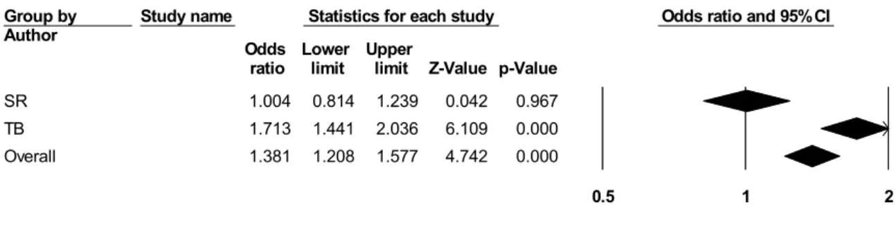
Figure 2 presents the outcome of the subgroup analysis based on participants’ first choices.
Figure 2. Subgroup analysis by authors
There is a marked contrast between the two groups, since, as Figure 2 shows, there is no overlap between the confidence intervals of the two groups. With the experiments by Steen et al., the summary effect size verges on 1, and the confidence interval of [0.814, 1.239] includes 1. This means that these experiments do not provide support for the research hypothesis that metaphors influence reasoning about crime. This group is quite homogenous in the sense that only about 14% of the observed variance reflects differences in the true effect sizes of the experiments (I2
= 14.221). In contrast, the experiments conducted by Thibodeau and Boroditsky have a summary odds ratio significantly higher than 1, and exhibit a very high degree of consistency (about 9% of the observed variance is real variance in true effect sizes, I2 = 8.949).
Accordingly, this group of experiments seems to provide support for the hypothesis that metaphors influence thinking about crime.
A Q-test based on analysis of variance reinforces our impression that the two groups are different. Namely, the difference between the groups is statistically significant: Qbetw = 14.833, df = 1, p = 0.0001. A fully random analysis (in which both the experiments within the groups, as well as the two groups themselves are combined with the help of a random-effects model) produces similar results, except that the confidence intervals are, of course, wider. Therefore, we may conclude that the variation of the true effect sizes pertaining to the first choice of participants might, to a large extent, be due to the different methods applied by the two groups of researchers.
4.4.2. Sub-group analysis – by political affiliation
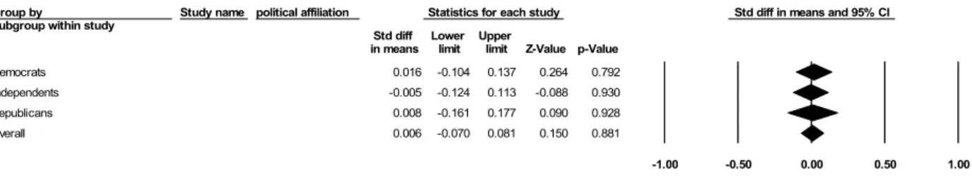
The variation in the effect sizes might be also due to factors which do not pertain to the peculiarities of the experiments as in the previous case, but to idiosyncrasies of subgroups within the participants in the experiments. Since political affiliation was one of the variables which were found to influence participants’ preferences for crime reduction measures in some experiments by the researchers who conducted them, it seems reasonable to check its impact with meta-analysis tools, too.7 Here again, a mixed-effects model seemed to be appropriate.
Figure 3 summarizes the results.
7 Christmann & Göhring (2016) does not include information about participants’ political affiliations, thus this experiment is excluded from this analysis.
Group by
Author Study name Statistics for each study Odds ratio and 95% CI
Odds Lower Upper
ratio limit limit Z-Value p-Value
SR 1.004 0.814 1.239 0.042 0.967
TB 1.713 1.441 2.036 6.109 0.000
Overall 1.381 1.208 1.577 4.742 0.000
0.5 1 2
frame-inconsistent frame-consistent
Meta Analysis
Figure3. Subgroup analysis with political affiliation as a variable
As Figure 3 shows, there is a considerable overlap among the three confidence intervals. And in fact, the comparison of the three groups yields that the between-studies Q-value is 3.690 with 2 as a degree of freedom and a corresponding p-value of 0.158. This means that there are no substantial differences among the three groups. Furthermore, the within-group variance in effects is significantly greater than the degree of freedom in the case of the Democrats, indicating a great amount of dispersion in the true effect sizes in this subgroup of participants.
As the corresponding I2-statistics indicate, about 44% of the observed variance in effect sizes cannot be attributed to random error but reflects differences in the true effect sizes of the experiments in this subgroup. In contrast to the Democrats and the Republicans, in the case of the Independents, a mean effect size significantly above 1 was obtained. Therefore, the metaphorical frame seemed to influence only this group of participants.8 To sum up, a subgroup-analysis based on the political affiliation of participants does not seem to be a good fit for the data.
4.5. Cumulative meta-analysis
Although the subgroup analysis by authors presented in Subsection 4.4.1 indicated that both groups of experiments produced highly consistent results, Figure 4 and 5 reveal an interesting feature of these experiments. Namely, with the experiments conducted by Thibodeau &
Boroditsky, the effect sizes gradually decrease. A cumulative meta-analysis reinforces this finding: if we calculate the summary effect size of these experiments stepwise in such a way that we always add an experiment and re-calculate the summary effect size, then we can see that it grows smaller over time.9 See Figure 4.
8 We have to add that the results of the Democrats were marginally significant.
9 Christmann & Göhring’s (2016) exact replication attempt is omitted from this analysis.
Group by
Subgroup within study Study name Political affiliation Statistics for each study Odds ratio and 95% CI Odds Lower Upper
ratio limit limit Z-Value p-Value
Democrats 1.337 0.986 1.813 1.870 0.061
Independents 1.418 1.046 1.922 2.250 0.024
Republicans 0.872 0.574 1.325 -0.641 0.521
Overall 1.252 1.034 1.516 2.298 0.022
0.5 1 2
Favours A Favours B
Meta Analysis
Study name Cumulative statistics Cumulative odds
ratio (95% CI) Lower Upper
Point limit limit Z-Value p-Value TB2011_1 2.151 1.451 3.188 3.812 0.000 TB2011_2 2.116 1.542 2.902 4.647 0.000 TB2011_4 2.154 1.620 2.863 5.284 0.000 TB2013_2 2.156 1.677 2.772 5.997 0.000 TB2013_3 2.142 1.688 2.717 6.275 0.000 TB2013_4 2.001 1.622 2.469 6.477 0.000 TB2015_1 1.783 1.471 2.161 5.891 0.000 TB2015_2 1.697 1.420 2.028 5.809 0.000 1.697 1.420 2.028 5.809 0.000
0.1 0.2 0.5 1 2 5 10
frame-inconsistent frame-consistent Meta Analysis
Figure 4. Cumulative meta-analysis – Thibodeau & Boroditsky
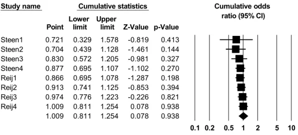
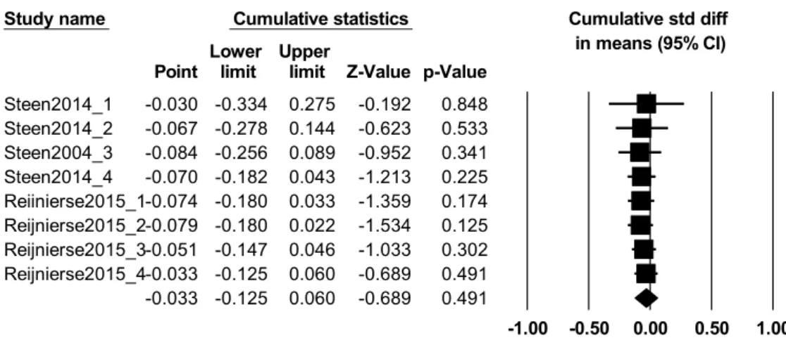
In contrast, as Figure 5 indicates, the cumulative summary effect size of the experiments conducted by Steen and his colleagues increased almost continuously:
Figure 5. Cumulative meta-analysis – Steen and his colleagues
Nonetheless, it is important to remark that the experiments Reij1-4 did not follow each other in a chronological order nor are they improved versions of each other. Rather, they originate from the same experiments (as the 1-4 metaphor conditions) – that is, they should be regarded as one data point.
To sum up, this might mean that there is a slight tendency to convergence between the results of the two rival camps. If we try to identify the cause if these trends, it is not the temporal relationships among the experiments which seems to be decisive but rather changes in the methodology applied by the researchers. This hypothesis is supported by the finding that the exact replication of Thibodeau & Boroditsky’s first experiment by Christmann and Göhring in 2016 yielded a higher effect size value than the original experiment.
4.6. The prediction interval
The 95% confidence interval of the summary effect size characterizes the precision of its estimate but does not provide information about the amount of the dispersion of the effect sizes.
Therefore, if we ask the question of whether a new experiment will have a true effect size falling between certain limits in 95% of the cases, then we have to calculate the prediction interval. This is always wider than the confidence interval. In this case, the prediction interval is [0.749, 2.648], as indicated by the red line in Figure 1. This means that the true effect size for any similar study will fall into this range in 95% of the cases, provided that the true effect sizes are normally distributed (while the true mean effect size will fall into the confidence interval of [1.165, 1.703] in 95% of the cases). That is, on the basis of the information included in these experiments, one cannot predict whether a similar experiment would indicate any effect of the metaphorical frame – a weak effect or no effect are similarly possible.
4.7. Publication bias
Study name Cumulative statistics Cumulative odds
ratio (95% CI) Lower Upper
Point limit limit Z-Value p-Value Steen1 0.721 0.329 1.578 -0.819 0.413 Steen2 0.704 0.439 1.128 -1.461 0.144 Steen3 0.830 0.572 1.205 -0.981 0.327 Steen4 0.877 0.695 1.107 -1.102 0.270 Reij1 0.866 0.695 1.078 -1.287 0.198 Reij2 0.913 0.741 1.125 -0.853 0.394 Reij3 0.974 0.776 1.223 -0.226 0.821 Reij4 1.009 0.811 1.254 0.078 0.938 1.009 0.811 1.254 0.078 0.938
0.1 0.2 0.5 1 2 5 10
frame-inconsistent frame-consistent Meta Analysis
Meta-analysis also includes tools for the estimation of possible publication bias. Publication bias usually results from the circumstance that experiments showing a significant result are more likely to be published than those indicating an insignificant result. Since experiments with a small number of participants produce significant results only if the effect size is large, they might remain unpublished more easily due to their low power. One method to check whether smaller studies with a negative outcome have been neglected is to examine the disposition of studies around the mean effect size. Large, medium-sized and smaller studies alike should be located symmetrically on the two sides of the mean effect size. Duval and Tweedie’s Trim and Fill method allows us to check this. In this method, the list of experiments is supplemented by fictional smaller experiments so that the symmetry is restored, and the summary effect size is re-calculated and compared to its original value.10
Duval and Tweedie’s trim and fill model indicates no missing study. This means that there is no evidence for publication bias resulting from missing small experiments.
5. Alternative analyses
The diversity of the data handling techniques applied by the researchers might motivate alternative analyses. The analysis presented in Sections 3 and 4 took into consideration only the top choices of participants. Nonetheless, there are other possibilities. In this section, we will discuss two of them.
5.1. The rankings/ratings analysis
The rankings/ratings analysis takes the rankings/ratings of the social reform-oriented vs. the enforcement-oriented measures into consideration. That is, while for the first (top choices) analysis, we needed data about the orientedness (social reform vs. enforcement) of the top choices in the beast and in the virus frames, respectively, for the second analysis data are needed about the whole range of the measures in the beast and in the virus frames, respectively.
5.1.1. The choice of the effect size indicator
The experiments can be divided into three groups in terms of the information they contain about participants’ evaluations of the measures. The data sheets belonging to Thibodeau &
Boroditsky (2013, 2015) and Steen et al. (2014) contain data about the ranking of the measures;
those by Reijnierse et al. (2015) include data about the rating of the measures; Christmann &
Göhring (2016) applied an open question task, thus their answer sheets make it possible to count the number of the social reform vs. enforcement-oriented answers given by each participant. In order to calculate the effect of the metaphorical frames on the evaluation of the measures, we can compare
– the means of the rankings of the social reform type/enforcement-oriented measures in the virus vs. beast condition;
– the means of the ratings of the social reform-type/enforcement-oriented measures in the virus vs. beast condition;
– the means of the number of the social reform-type/enforcement-oriented measures in the virus vs. beast condition.
10 See Borenstein (2009: Section 30) on this.
This data type motivates the use of the effect size indicator standardized mean difference, i.e.
Cohen’s d. Cohen’s d is calculated in such a way that the difference of the sample means in the two conditions is divided by the within-group standard deviation pooled across conditions. In contrast to the odds ratio, the null-value (neutral value) is 0. That is to say, d = 0 indicates that there is no difference between the rankings/ratings/number of items in the two conditions (metaphorical frames). According to Cohen’s recommendation, a d value of 0.2 indicates a small effect; 0.5 indicates a medium effect; 0.8 means a large effect. A negative value shows that there is an effect in the opposite direction – i.e. participants rank/evaluate frame- inconsistent measures higher.
5.1.2. Methods of data collection
Similarly to the first analysis presented in Sections 3-4, data had to be extracted and computed from the information in the data sheets. For details of this process, as well as the means and standard deviations of the individual experiments, see the Open Science Framework page https://osf.io/gwaj6/?view_only=b1013469554e409684b258c81666f105.
5.1.3. The effect size of the individual experiments
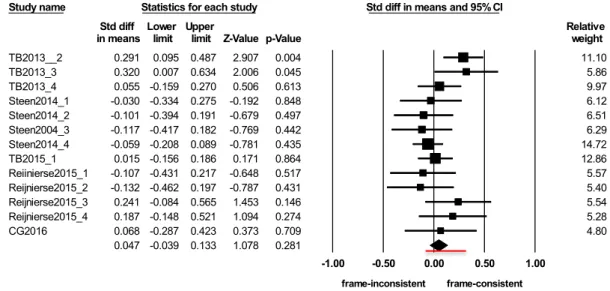
Figure 6 shows the individual effect sizes, their confidence intervals, Z-values, p-values, and weights.
Figure 6. Effect sizes of the experiments and the summary effect size in the complex analysis
The standardized mean difference of the individual experiments ranged from -0.132 (Reijnierse et al., 2015, 2-metaphor condition) to 0.32 (Thibodeau & Boroditsky 2013, Experiment 3). In contrast to the first analysis (top choices), only 7 experiments out of 13 indicated an effect of the metaphorical frames, i.e., provided a positive SMD. This could suggest the opposite conclusion to the previous case. A decision on the basis of these pieces of information, however, would be unfounded, too. We have also to take into consideration that in the second analysis, there were only 2 experiments for which the confidence interval did not include the value 0. Thus, the majority of the experiments did not provide a significant result, and the confidence intervals ranged from -0.462 to 0.634, which yields a rather wide spectrum.
Study name Statistics for each study Std diff in means and 95% CI
Std diff Lower Upper Relative Relative
in means limit limit Z-Value p-Value weight weight
TB2013__2 0.291 0.095 0.487 2.907 0.004 11.10
TB2013_3 0.320 0.007 0.634 2.006 0.045 5.86
TB2013_4 0.055 -0.159 0.270 0.506 0.613 9.97
Steen2014_1 -0.030 -0.334 0.275 -0.192 0.848 6.12
Steen2014_2 -0.101 -0.394 0.191 -0.679 0.497 6.51
Steen2004_3 -0.117 -0.417 0.182 -0.769 0.442 6.29
Steen2014_4 -0.059 -0.208 0.089 -0.781 0.435 14.72
TB2015_1 0.015 -0.156 0.186 0.171 0.864 12.86
Reiinierse2015_1 -0.107 -0.431 0.217 -0.648 0.517 5.57
Reijnierse2015_2 -0.132 -0.462 0.197 -0.787 0.431 5.40
Reijnierse2015_3 0.241 -0.084 0.565 1.453 0.146 5.54
Reijnierse2015_4 0.187 -0.148 0.521 1.094 0.274 5.28
CG2016 0.068 -0.287 0.423 0.373 0.709 4.80
0.047 -0.039 0.133 1.078 0.281
-1.00 -0.50 0.00 0.50 1.00
frame-inconsistent frame-consistent
Meta Analysis
5.1.4. Synthesis of the results
Similarly to the first (top choices) analysis, the application of the random effect model is appropriate in this case, too. As the last row of Figure 6 shows, the summary effect size of 0.047 is not significant; Z = 1.078, p = 0.281. Its confidence interval [-0.039, 0.133] includes the value 0, and overlaps with the majority of the confidence intervals of the individual experiments. This confidence interval is very narrow, indicating a very precise estimation of the summary effect. From these results we can conclude that the experiments together do not provide evidence for Thibodeau and Boroditsky’s research hypothesis in this case.
As for the consistency of the effect sizes, the Q-value, i.e. the total amount of the observed between-experiments variance is 17.409. Its expected value is df(Q) = 12. These two values are not significantly different from each other, p = 0.135. This means that the total variation is not significantly greater than the sum of the within-study variations, suggesting that these experiments might share a common true effect size. The second relevant indicator is the estimate for the standard variation of the true effects, denoted as T2. This is 0.007 in log units with a standard error of 0.01. This means that the standard deviation of the true effects, i.e. T, is 1.09. Finally, the I2 value is 31.068, which means that about 31% of the observed variance in effect sizes cannot be attributed to random error but reflects differences in the true effect sizes of the experiments. This indicates a rather small amount of variation in the true effect sizes in this case.
The prediction interval is [-0.163, 0.256]. This means that the true effect size for any similar study will fall into this range in 95% of the cases, provided that the true effect sizes are normally distributed. That is, we may expect a result indicating no or a weak effect.
The first reaction to the discrepancy between the two analyses might be that the reason for the first analysis (top choices) yielding a higher summary effect size could be the fact that it includes 8 experiments by Thibodeau & Boroditsky, while the second analysis (ratings/rankings) only includes 4. Undeniably, this is a factor that has a major influence on the summary effect size. To wit, if we omit Experiments 1, 2, and 4 of Thibodeau & Boroditsky (2011) and Experiment 2 of Thibodeau & Boroditsky (2015) from the first analysis, a random effects model yields 1.260 as the summary effect size with a confidence interval of [1.019, 1.557]. But there is a second factor, too, which seems to be more interesting. Namely, if we compare the effect sizes of the individual experiments by transforming the odds ratios into standardized mean difference, we get the following picture. See Table 5.11
experiment top choices ratings/rankings
TB2013/2 0.426 0.291
TB2013/3 0.388 0.320
TB2013/4 0.251 0.055
Steen2014/1 -0.181 -0.030
Steen2014/2 -0.201 -0.101
Steen2014/3 0.048 -0.117
Steen2014/4 -0.053 -0.059
TB2015/1 0.120 0.015
Reijnierse/1 -0.139 -0.107
Reijnierse/2 0.233 -0.132
Reijnierse/3 0.301 0.241
Reijnierse/4 0.200 0.187
CG2016 0.450 0.068
Summary effect size 0.127 0.047
11 In the case of the experiments in Reijnierse et al. (2015), the value of the complex analysis is computed as the average of the effect size of the social reform-type answers and the enforcement-type answers.