A Graph Solver for the Automated Generation of Consistent Domain-Specific Models

(1)

Consistent Domain-Specific Models

Oszkár Semeráth

^1,2

, András Szabolcs Nagy

^1,2

and Dániel Varró

^3,1,2

1MTA-BME Lendület Cyber-Physical Systems Research Group, Hungary

2Budapest University of Technology and Economics, Department of Measurement and Information Systems, Hungary

3McGill University, Canada

semerath@mit.bme.hu,nagya@mit.bme.hu,varro@mit.bme.hu

ABSTRACT

Many testing and benchmarking scenarios in software and systems engineering depend on the systematic generation of graph models.

For instance, tool qualification necessitated by safety standards would require a large set of consistent (well-formed or malformed) instance models specific to a domain. However, automatically generating consistent graph models which comply with a metamodel and satisfy all well-formedness constraints of industrial domains is a significant challenge. Existing solutions which map graph models into first-order logic specification to use back-end logic solvers (like Alloy or Z3) have severe scalability issues. In the paper, we propose a graph solver framework for the automated generation of consistent domain-specific instance models which operates directly over graphs by combining advanced techniques such as refinement of partial models, shape analysis, incremental graph query evaluation, and rule-based design space exploration to provide a more efficient guidance. Our initial performance evaluation carried out in four domains demonstrates that our approach is able to generate models which are 1-2 orders of magnitude larger (with 500 to 6000 objects!) compared to mapping-based approaches natively using Alloy.

ACM Reference Format:

Oszkár Semeráth^1,2, András Szabolcs Nagy^1,2and Dániel Varró^3,1,2. 2018. A Graph Solver for the Automated Generation of Consistent Domain-Specific Models. InProceedings of ICSE ’18: 40th International Conference on Software Engineering , Gothenburg, Sweden, May 27-June 3, 2018 (ICSE ’18),12 pages.

https://doi.org/10.1145/3180155.3180186

ACKNOWLEDGMENTS

This paper is partially supported by MTA-BME Lendület Cyber- Physical Systems Research Group, the NSERC RGPIN-04573-16 project and the UNKP-17-3-III New National Excellence Program of the Ministry of Human Capacities. We are grateful for Alexandra Sólyom and Gábor Szárnyas for preliminary experiments in using design space exploration for model generation and all contributors to past model generators of query and transformation benchmarks.

Permission to make digital or hard copies of part or all of this work for personal or classroom use is granted without fee provided that copies are not made or distributed for profit or commercial advantage and that copies bear this notice and the full citation on the first page. Copyrights for third-party components of this work must be honored.

For all other uses, contact the owner/author(s).

ICSE ’18, May 27-June 3, 2018, Gothenburg, Sweden

ACM ISBN 978-1-4503-5638-1/18/05.

https://doi.org/10.1145/3180155.3180186

1 INTRODUCTION

Motivation.The automated generation of graph models has re- cently become a key approach in various application areas of software and systems engineering. Representing objects and pointers as graphs in object-oriented programs, automatically generated models may serve as complex test stubs [1, 2]. Auto-generated graphs help the testing and benchmarking of graph databases [3] since obtaining real graphs from business use cases is often difficult to due to protection of intellectual property rights. Automated synthesis of prototypical test contexts [4] aims to systematically derive previously unanticipated contexts in the form of graph models for the assurance of smart cyber-physical systems (CPS).

Similarly, in many design and verification tools used for engineering complex CPSs, system models are also represented internally as graphs, and model generators may be used for validating, testing or benchmarking such design tools [5–8]. As a main practical motivation for this scenario, while tool qualification of design and verification tools are necessitated by safety standards (like DO- 178C [9], or ISO 26262 [10]), tool qualification is extremely costly due to the lack of effective best practices for validating the tools themselves. Considering tool qualification as a long-term objective, our approach will be illustrated in the context of an industrial domain-specific modeling tool (Yakindu Statecharts), but it could be adapted to many other practical scenarios above.

In [11], four desirable properties are stated as key challenges for graph model generators used in such scenarios. A set of auto- generated graphs should ideally be (1)consistent, i.e. each graph should satisfy all well-formedness (WF) constraints, (2)diverse, i.e. each pairs of graphs should be structurally distant from each other, (3)scalable, i.e. the size of models are exponentially growing, and (4)realistic, i.e. auto-generated graphs cannot be distinguished from real models created by engineers by using advanced graph metrics [3, 12, 13]. For instance, characteristics (1,2) are essential in a functional testing scenario, while properties (3,4) are crucial for benchmarking and stress testing.

However, real models created by engineers are dominantly consistent (see [11] for a statistical analysis) according to the correct- by-construction principle (e.g. commits are disallowed when test cases fail or constraints are violated). Similarly, auto-generated graphs violating a single WF constraint but satisfying all the others are frequently necessitated for testing purposes. Moreover, random generation of graphs is unable to guarantee consistency, i.e. many WF constraints will be violated. This way, thesynthesis of consistent graphs is a prerequisite of both realistic and diverse graph models.

Problem Statement.This paper aims to automatically generate well-formed graph models of a specification defined by (1) a

(2)

metamodel (graph schema), (2) a set of well-formedness (WF) constraints expressed in first-order graph logic with transitive closure and optionally (3) an initial model fragment. Existing approaches like [14–20] map the instance generation problem of consistent graph models into logic solvers such as Alloy [21, 22], SMT-solvers [23], SAT-solvers or constraint solvers when the efficiency of graph model generation depends on the scalability and performance of back-end logic solvers, which primarily excel infinding inconsistencies in complex specifications. However, the generation models as a side-effect of the proof construction is much less efficient.

In fact, these solvers guarantee neither scalability [24] nor diversity [25] when they need to generate well-formed graph instances of a specification – regardless of how smart the mapping is from a high- level graph model to the underlying logic solver. From a practical perspective, while the specification of complex industrial modeling tools may contain hundreds of classes (in their metamodel) and WF constraints, no existing model generation technique could derive a consistent graph that contains at least one object from each class.

Contribution.We propose a novel automatic generation technique to derive consistent domain-specific graph models for specifications by exploiting and innovatively combining a multitude of advanced graph-based and core SAT-solving techniques.

(1) We formulate model generation as arefinement of partial models[26, 27] where initial abstract model fragments are gradually refined and concretized during exploration.

(2) We providepartial model refinement rulesasdecisionandunit propagationsteps by following core SAT-solving techniques.

(3) We use incremental graph query evaluation of the VIATRA engine [28] to efficientlyevaluate violations of constraints over partial modelsduring model generation [27].

(4) We integrateshape analysis as state encoding[29–31] for graphs to efficiently detect if two partial models should be treated as equivalent during exploration.

(5) We exploit rule-based design space exploration [32] todrive the generation process directly over graph shapesusing an objective function approximating the distance from a solution.

(6) Weevaluate the scalability of our approachusing 6 tests sets of four domains (including industrial DSLs) and compare its performance with the well-known Alloy Analyzer [21].

Added Value.To our best knowledge, our framework is one of the first attempts to automatically generate consistent models by operating natively over (typed and attributed) graphs. Moreover, according to our scalability experiments, it is capable ofgenerating consistent graph models of 1-2 orders of magnitude larger(with 500- 6000 nodes) compared to models derived by Alloy and the generated model suite is also more diverse [24]. As such, our graph solver can serve as a back-end where Alloy was used previously for model generation purposes in testing and benchmarking scenarios.

2 MODELING PRELIMINARIES

Our model generation technique will be illustrated by automatically generating test inputs for Yakindu Statecharts Tools [33], which is an industrial integrated modeling framework for developing reactive, event-driven systems. First, we give a brief introduction to the formal definition of partial models using a three-valued logic, which will drive the automated generation of consistent models.

2.1 Metamodels

A domain-specific (modeling) language (DSL) is typically defined by ametamodeland a set ofwell-formedness constraints. A metamodel defines the main concepts and relations in a domain, and specifies the basic graph structure of the models, and WF constraints further restrict valid models of the language by defining additional design rules. In this paper, the Eclipse Modeling Framework (EMF) [34] is used for domain modeling, which is a de facto industrial standard.

Pseudostate

Vertex Region

Transition

Statechart

Entry Synchronization State

RegularState CompositeElement [0..*] vertices

[0..*] regions [1..1] target

[0..*] incomingTransitions

[0..1] source [0..*] outgoingTransitions

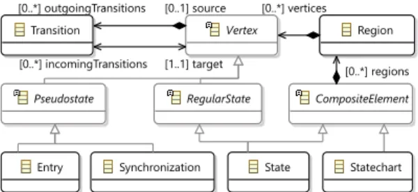
Figure 1: Metamodel of Yakindu statecharts

Example 2.1. A metamodel extracted from Yakindu is illustrated in Figure 1. AStatechartconsists ofRegions, which in turn contain Vertexes andTransitions. An abstract stateVertexis further refined intoRegularStates (likeState) andPseudoStates likeEntryand Synchronizationstates. The source and target states of a transition are identified by thesourceandtargetreferences.

To reason about the consistency of DSLs, a formal algebraic specification is frequently created [19, 27, 35–38]. We briefly revisit the notation of [27] to provide a precise background for our model generation approach (but for space consideration, we omit the detailed handling of attributes, which could be introduced accordingly).

Formally, a metamodel defines a vocabularyΣ={C1, . . . ,Cn, exist,R₁, . . . ,R_m,∼}with unary predicate symbolsC_i(1≤i≤n) defined for eachEClass, and binary predicate symbolsR_j (1≤j≤ m) for eachEReference. To represent abstract (partial) models, a unaryexistpredicate is introduced to denote the existence of an object in a given model, while∼denotes an equivalence relation over objects.

2.2 Partial Models

Partial models (PM) were introduced in [35, 38] to represent uncertain (possible) elements in instance models where one partial model represents a range of possible instance models. In this paper, 3-valued logic [39] is used to explicitly represent unspecified or unknown properties of models with a third¹/2truth value (be- sides 1 and 0 which stand fortrueandfalse) in accordance with [11, 27, 31]. Apartial modelis represented as a 3-valued logic struc- tureP=⟨Obj_P,I_P⟩ofΣ, whereObj_Pis the finite set of individuals in the model (i.e. the objects), andI_P provides a 3-valued interpretation for all constants inIdand predicate symbols inΣ.

Type Predicates.I_Pis a 3-valued interpretation of each class sym- bolC_iinΣ:I_P(C_i):Obj_P → {1,0,¹/2}: 1, 0 and¹/2means that it is true, false or unspecified if an object is an instance of a classCi. Reference Predicates.I_P gives a 3-valued interpretation to each reference symbolR_jinΣ:I_P(R_j):Obj_P×Obj_P→ {1,0,¹/2}, where

(3)

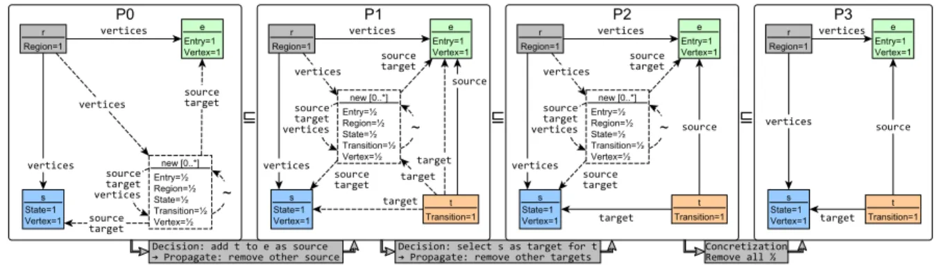
Figure 2: Sample partial models with uncertain elements and their refinement

1, 0 and¹/2means that it is true, false or unspecified if there is a referenceR_jbetween two objects.

Existence Predicate.I_P gives a 3-valued interpretation for the existence predicateI_P(exist) : Obj_P → {1,0,¹/2}, where 1 values represent an object that must be,¹/2value represents objects that may be included in a model.

Equivalence Predicate.I_Pgives a 3-valued interpretation to the

∼relation between the objectsI_P(∼):Obj_P×Obj_P → {1,0,¹/2}. An uncertain¹/2value relation between two objects means that those object may be equal and can potentially be merged. On the other hand, uncertain equivalence of a single object (with itself) implies that it may represent multiple separate objects.

Example 2.2. Four partial models are illustrated in Figure 2. As a notation guide, (1) the truth value of atype predicateis denoted by labels on nodes, where missing labels are treated as 0 values, while (2)reference predicatevalues 1 and¹/2are represented by edges with solid and dashed lines (respectively), while missing edges between two objects represent 0 values for a predicate, (3)existence predicatevalues 1 and¹/2are represented by nodes with solid and dashed borders, respectively, while objects with 0 existence values are simply not depicted. Finally, (4) uncertain¹/2equivalences are marked by dashed line with an∼symbol. Otherwise, each node represents a single, unique object (i.e. for all objecto:[[o∼o]]=1 and for all different objectso1ando2:[[o1∼o2]]=0).

InP0(on the left side of Figure 2), objectris of typeRegionbut not of typeState:[[Region(r)]]^P⁰=1 and[[State(r)]]^P⁰=0. In case of objectnew, all type predicate are¹/2, which means that the object may represent any type of objects. InP0there is a certainvertices reference betweenrandsandr ande, and a possible reference betweenrandnewor as a self-loop ofnew. Nodesr,eandsrepresent objects that must exist, andnewrepresent possible objects which may exist or they might be removed later from the model. Node newmay also represent multiple objects (note the self-loop edge∼), which can later be refined into multiple distinct model elements.

2.3 Refinement and Concretization of PMs

During model generation, the level of uncertainty will gradually be reduced byrefinementsderiving partial models that represent more concrete instance models. In a refinement step, properties with¹/2

values can be refined to either 0 or 1 which imposes an information ordering relationX ⊑Ywhere eitherX =¹/2andYis refined to 1 or

0, or values ofXandY remain equal:X ⊑Y:=(X =¹/2) ∨ (X =Y). A refinement is defined as a functionref :Obj_P →2^Obj^Q which maps each object of a partial modelP to a set of objects in the refined partial modelQ. A refinement respects the information ordering of type, reference, equivalence and existence predicates for eachp1,p2∈Obj_Pandq1∈ref(p1),q2∈ref(p2):

• for each classC_i:[[C_i(p₁)]]^P ⊑ [[C_i(q₁)]]^Q.

• for each referenceR_j:[[R_j(p1,p2)]]^P ⊑ [[R_j(q1,q2)]]^Q

• [[p1∼p2]]^P ⊑ [[q1∼q2]]^Q

• [[exist(p1)]]^P ⊑ [[exist(q1)]]^Q, and if[[exist(p)]]^P =1 then ref(p)is not empty

Refinement from partial modelPtoQis denoted byP⊑Q.

If a 3-valued partial modelPonly contains 1 and 0 values, and there are no∼relations between different objects (i.e. all equivalent nodes are merged), thenPrepresents a traditionalinstance model.

Aconcretizationdefines a trivial refinement to a 2-valued fully defined concrete model by rewriting all¹/2type, reference and exist predicates values to 0, and rewriting all¹/2equivalence predicate to 0 between different objects, and to 1 on the same object.

Example 2.3. Figure 2 illustrates two refinement steps fromP0

toP2. InP1objectnewis split into two different objects:newand tofP1, where[[new∼new]]^P⁰=¹/2is refined to[[new∼t]]^P¹=0, [[t∼t]]^P¹=1 and[[new∼new]]^P¹=¹/2. Additionally,[[exist(new)]]^P⁰

=¹/2is refined to[[exist(t)]]^P¹=1, and[[Transition(new)]]^P⁰ =¹/2

is refined to[[Transition(t)]]^P¹=1, thus creating a newTransition objectt, while all other¹/2type predicates are refined to 0. Finally, sourcepredicates are refined to 1 witheas target, and to 0 with all other objects as target.

In stepP1toP2, possibletargetpredicates are refined to 1 with sas target object, and to 0 witheandnewas target objects. Note that refinement stepP1⊑P2will illustrate the decision rule while P₂⊑P₃will illustrate the unit propagation rule later in section 3.1.

P3is a concretization ofP2, which is also a refinementP2⊑P3.

2.4 Defining constraints over PMs

In many industrial modeling tools, domain-specific WF constraints are captured either by standard OCL constraints [40] or by graph patterns (GP) [28, 41]. A graph pattern captures complex structural conditions over an instance model. In order to have a unified and

(4)

[[C(v)]]^P_Z:=I_P(C)(Z(v)) [[R(v₁,v₂)]]^P_Z:=I_P(R)(Z(v₁),Z(v₂))

[[exist(v)]]^P_Z:=I_P(exist)(Z(v)) [[v1∼v2]]^P_Z:=I_P(∼)(Z(v1),Z(v2)) [[φ₁∧φ₂]]^P_Z:=min([[φ₁]]^P_Z,[[φ₂]]_Z^P) [[φ1∨φ2]]^P_Z:=max([[φ1]]^P_Z,[[φ2]]_Z^P)

[[¬φ]]^P_Z:=1− [[φ]]^P_Z

[[∃v:φ]]^P_Z:=max{[[exist(x) ∧φ]]^P_Z,v↦→x:x∈Obj_P} [[∀v:φ]]^P_Z:=min{[[¬exist(x) ∨φ]]^P_Z,v_↦→_x:x ∈Obj_P} [[φ⁺(v1,v2)]]^P_Z:=[[φ(v1,v2) ∨ (∃m:φ(v1,m) ∧φ⁺(m,v2))]]^P_Z

Figure 3: Semantics of graph logic expressions

semantically precise handling of evaluating graph patterns constraints for regular and partial models, we use a first-order graph logic formalism with transitive closure that covers the key features of several concrete graph pattern languages. This semantics was introduced in [27] being influenced by [31].

Syntax.A graph pattern is a first order logic predicate with transitive closureφ(v1, . . . ,v_n) over (object) variables. A graph predicateφcan be inductively constructed by using object variable symbols (v1,v2, . . .), atomic predicates (C(v),R(v1,v2),v1∼v2), standard logic connectives (¬,∨,∧), logic quantifiers (∃and∀), and transitive closure over binary predicates denoted asφ⁺(v1,v2).

Semantics.A predicateφ(v₁, . . . ,v_n)can be evaluated on partial modelPalong a variable bindingZ, which is a mappingZ :

{v1, . . . ,v_n} → Obj_P from variables to objects inM. The truth

value ofφcan be evaluated over a partial modelPandZ(denoted by[[φ(v1, . . . ,vn)]]^P_Z) in accordance with the semantic rules defined in Figure 3. Note thatminandmax takes the numeric minimum and maximum values of 0,¹/2and 1, and the rules follow 3-valued interpretation of standard logic formulae as defined in [27, 31]. A variable bindingZwhere the predicateφis evaluated to 1 overPis called apattern match, formally[[φ]]^P_Z =1.

Graph predicates are frequently used for defining complex structural WF constraints and validation rules [28]. In such a case,a predicate match denotes a constraint violation, thus the correspond- ing graph formula needs to capture the erroneous cases, and a match detect a violation of a WF constraint. Therefore, a set of WF predicates{φ^WF₁ , . . . ,φ^WF_n }defines a theorem of valid modelsT, whereT ={¬φ^WF₁ , . . . ,¬φ^WF_n }. WF predicates ofT are derived from two sources: the metamodel defines the basic structure, and additional validation constraints of a domain can be defined by using OCL [40] or graph patterns [28].

There are structural constraints imposed by the underlying graph representation. In case of EMF metamodels, such constraints include (1)Type Hierarchy (TH)which expresses that a more specific (child) class has every structural feature of the more general (parent) class, (2)Type Compliance (TC)that requires that for any relation R(o,t), its source and target objectsoandtneed to have compliant types, (3)Abstract (ABS): If a class is defined as abstract, it is not allowed to have direct instances, (4)Multiplicity (MUL)of structural features can be limited with upper and lower bound in the form of “lower..upper” and (5)Inverse (INV), which states that two parallel references of opposite direction always occur in pairs. Finally

noOutgoing(e):=

Entry(e) ∧ ¬∃t1,t2,e1,s: source(t1,e1) ∧target(t2,s)

∧e∼e1∧t1∼t2

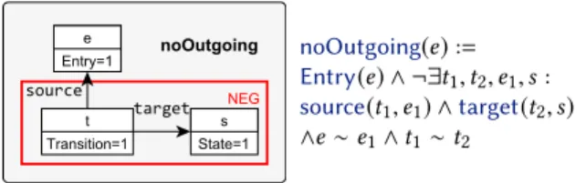
Figure 4: Sample statechart WF constraint as graph query

instance models in EMF are expected to be arranged into a (6)Con- tainment (CON)hierarchy, which is a directed tree along relations marked in the metamodel as containment (e.g.regionsorvertices).

Since a formalization of these structural restrictions as WF constraints is provided in [19], the graph predicate language of Figure 3 can uniformly be used for both kinds of structural constraints.

Example 2.4. The Yakindu documentation states several constraints for statecharts that can be formalized as graph predicates [24]. For instance, constraintnoOutgoing(e)in Figure 4 (depicted as a graph pattern and a graph predicate) detects an entry stateewith- out an outgoing transition. The explicit use of equality constraints e ∼e₁andt₁∼t₂is responsible for performing a natural join op- eration over the edges as predicates. As a result, the same formula can be evaluated with both 2-valued and 3-valued interpretation.

2.5 Approximating constraints over PMs

While WF constraints can be directly evaluated on concrete instance models, checking the correctness of a partial model is a challenging task, because one partial model may represent multiple concretiza- tions. A constraintφcan be evaluated on a partial modelPusing the 3-valued logic and open-world semantics by a constraint rewriting technique [27] which over- and under-approximates the results:

• Under-Approximation: If[[φ]]^P =1 in a partial modelP, then[[φ]]^Q=1 in any partial modelQwhereP⊑Q.

• Over-ApproximationIf[[φ]]^Q = 1 in a partial modelQ, then[[φ]]^P ≥¹/2in a partial modelPwhereP⊑Q.

Using these properties, we define a monotonous derivation sequence of valid partial models which (1) starts from the most abstract partial model where all constraints are evaluated to¹/2, which partial model (2) is gradually refined into more and more concrete partial models (with less number of predicates evaluating to¹/2).

Refinement steps are continued until a concretized graph model of a designated scope eventually satisfies all WF constraints with 2-valued interpretation. During these refinement steps, special care needs to be taken to handle two situations:

• False negativesare partial modelsPwhich do not violate an under-approximated (must) constraint, i.e.[[φ]]^P ≤ ¹/2, but they can never be concretized into a valid instance model with[[φ]]^Q =0 whereP⊑Q. These sequences are dead ends, and ideally, they should be detected as early as possible.

• False positivesare partial modelsPwhich violate an over- approximated (may) constraint, i.e.[[φ]]^P ≥ ¹/2, but they can be further refined into partial model[[φ]]^Q =0 where P⊑Q. These sequences might be postponed during model generation, but they may eventually lead to a concrete model that satisfies all WF constraints, thus they should be kept.

(5)

Our graph generation approach will derive instance models along refinements. As such, partial models will gradually become more and more concrete after each refinement step which implies that checking WF constraints on partial models also becomes more precise. The practical benefit compared to consecutive calls to back- end solvers [24] is that the complex model finding problem can be divided into a sequence of small decisions while WF constraints can be checked (approximately) on intermediate solutions.

3 AUTOMATED GRAPH GENERATION

In this paper, we propose a general and automated graph model generation approach which takes a domain specified by (I1) a vo- cabularyΣdefined by a metamodel, and (I2) a theoremTdefined by a set of well-formedness constraints{¬φ₁^WF, . . . ,¬φ_n^WF}, and (I3) a search scope (i.e. minimal and maximal number of nodes in a solution graph) and (O) generates a consistent (valid) concrete graph modelG|=Tas output.

The model generation framework gradually refines partial models by rule-based design space exploration (DSE) [32] into a well- formed instance model which complies to the metamodel and all WF constraints are satisfied, if such a concrete model exists within the given search scope. During exploration, our framework simultaneously operates on (concrete) instance models and WF constraints as well as (abstract) partial models and approximated WF constraints introduced in section 2 by applying refinement rules.Refinement rulesare defined as graph transformation rules [27, 42] manipulat- ing directly over partial models with 3-valued interpretations by concertizing a single atomic uncertain¹/2value in each step.

Refinement rules are grouped into two categories: (1)Decision rulesare derived fromΣto reduce the number of valid concretiza- tions of a partial model (i.e. new information is added) while (2) Unit propagation rulesare derived fromT to propagate the consequences of previous decisions in order to simplify a solution candidate without excluding potential solutions.

Model generation is initiated from aninitial partial modelpro- vided as input by an engineer, or from themost abstract partial model where all predicates are unknown, i.e. (1) there is a single (abstract) objectObj_P ={new}; (2)exist(new)=¹/2andnew∼new=¹/2thus this object may represent multiple possible objects of the concrete models; (3) for all class predicateC_i:C_i(new)=¹/2; and (4) for all reference predicatesR_j:R_j(new,new)=¹/2.

3.1 Decision Rules

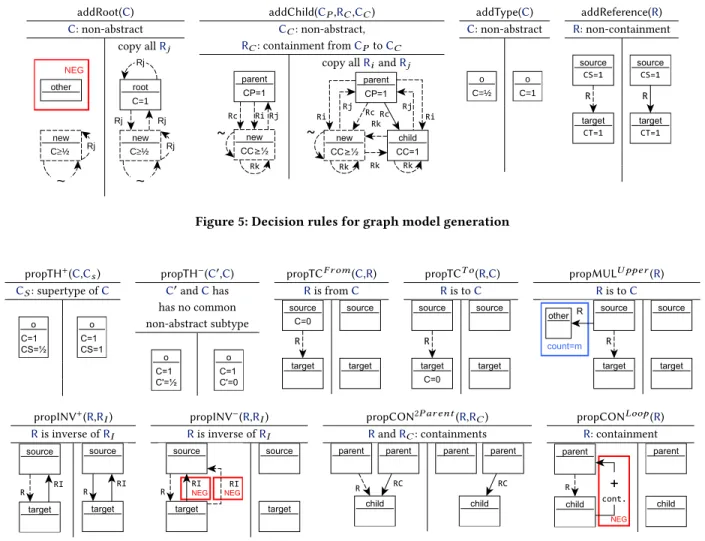
Decision rules (see Figure 5) define various refinements to con- cretize information in partial models to construct possible solutions.

They are derived from the vocabularyΣof the metamodel, where each predicate symbolC_iandR_j represents aClassandReference.

In general, decision rules are responsible for (1) introducing new objects by splitting the abstractnewobject or (2) rewriting an¹/2

value to 1 as detailed by (the scheme of) four decision rule classes.

•RuleaddRoot(C)selects a non-abstract classC(see the pre- condition in the left hand side) if no other roots have been created (denoted byNEG) to ensure that the model has a single root (as required by EMF). Its effect (prescribed by the right hand side) is to split the initialnewobject by creating a newrootas an instance ofC, which acts as a root element

for the containment hierarchy and all self-loop references onneware extended to both objects.

• RuleaddChild(C_P,R_C,C_C)selects an existingparentobject of typeC_P, thenewobject with a non-abstract typeC_C, and a containment referenceR_Cfromparenttonew. Upon execution, it splitsnewinto a new objectchildof typeC_C connected toparent viaR_C, thus unfolding a new object along the containment hierarchy. During the unfolding step, all outgoingR_i, incomingR_j and loopR_kreferences ofnew are extended (copied) tochild.

• Finally, two rulesaddType(C)andaddReference(R)refine uncertain¹/2classes and references in the partial model. In the latter case, the rule requires that the types of the endpoints are already fixed appropriately.

Example 3.1. The refinement stepP0⊑P1in Figure 2 introduces a new objecttby applying thedecision ruleaddChild(of Figure 5), which changes¹/2values oftransition(t)andsource(t,e)to 1.

3.2 Unit Propagation Rules

Unit propagation rules are responsible for refining unspecified elements in a partial model without excluding any valid solution to simplify the partial model propagating the consequences of previously applied decision rules. Unit propagation rules are applied repeatedly right after a decision rule is applied. They are derived from the structural constraints (1)-(6) introduced in section 2.4. In general, unit propagation rules rewrite¹/2elements to 0 (or 1) if a 1 (or 0) value would contradict to a constraint. Figure 6 illustrates (the scheme of) unit propagation rules used in this paper.

• Type hierarchy (TH)is maintained by two rules:propTH⁺(C,C_s) propagates a positive (1) type predicate ofCto a supertype Cs;propTH⁻(C^′,C)rewrites a¹/2type predicate value to 0 for typeCif the object already has an incompatible typeC^′ whereCandC^′do not have a common subclass (all classes are considered to be subclasses of themselves).

• Type compliance (TC)is checked by two rules:propTC^{F rom}(C,R) andpropTC^{T o}(R,C). Both rules remove possible references if the types of the reference end-points are incompatible.

• RulepropMUL^{U pper}(R)checks theupper multiplicity (MUL) of a reference, and removes all possible additional links if the upper limit is reached.

• TheInverse (INV)structural constraint is checked two rules:

propINV⁺(R,R_I)andpropINV⁻(R,R_I)which set aRpredicate value to 1 or 0 if an inverseR_I value is already set.

• To ensureContainment hierarchy (CON), first decision rules enforce that each non-root object has a parent. Then, additional possible incoming containment references are removed by unit propagation rulepropCON^{2Par ent}(R,R_C).

Finally,propCON^Loop(R)removes possible reference predicates that would create a loop in the containment hierarchy.

Decision and unit propagation rules are in close analogy with the DLL62 algorithm of traditional SAT-solvers [43]: values of variables are graph elements in our case (instead of Boolean values), complex graph predicates are evaluated (instead of conjunctive normal formulae), and the state space of graphs needs to be continuously stored during exploration (instead of a search tree).

(6)

addRoot(C) C: non-abstract

copy allR_j

new C≥½ other

NEG

Rj

~

root C=1

new C≥½ Rj

Rj

~

Rj

addChild(C_P,R_C,C_C) C_C: non-abstract, RC: containment fromCPtoCC

copy allRiandRj

addType(C) C: non-abstract

o C=½

o C=1

addReference(R) R: non-containment

Figure 5: Decision rules for graph model generation

propTH⁺(C,Cs) CS: supertype ofC

propTH⁻(C^′,C) C^′andChas has no common non-abstract subtype

propTC^{F r om}(C,R) Ris fromC

propTC^{T o}(R,C) Ris toC

propMUL^{U ppe r}(R) Ris toC

propINV⁺(R,RI) Ris inverse ofRI

propINV⁻(R,RI) Ris inverse ofRI

propCON^{2P ar e nt}(R,RC) RandRC: containments

propCON^Loop(R) R: containment

Figure 6: Unit propagation rules for graph model generation

Example 3.2. Refinement stepP1⊑P2is a result of adecision rule addChildto set the¹/2value oftarget(t,s)to 1 followed by aunit propagation rulepropMUL^{U pper}(target)which aims to prevent the partial model from violating an upper multiplicity constraint by setting¹/2values oftarget(t,e)andtarget(t,new)to 0 as a direct consequence of the previous decision rule.

As a preprocessing step, decision and propagation rules are derived. Moreover,under-approximated (must) predicatesare synthesized from graph predicates in accordance with [27] to detect unre- solvable WF constraints early in a partial solution.

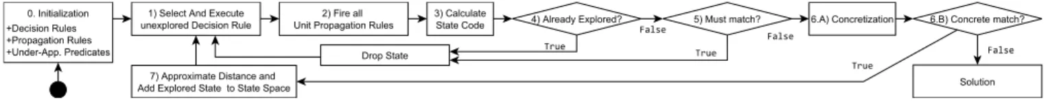
3.3 Exploration

During exploration (see Figure 7), refinement rules are repeatedly applied driven by an objective function and a rule selection strategy.

As such, the size of partial models is continuously growing up to the designated scope, while the number of uncertainties and constraint violations in these partial models are decreasing to ensure that the process converges to consistent instance models. Now we discuss the steps of the model generation process.

(1)After initializing the search with an initial partial model, an unexplored decision rule is selected and appliedto derive a new (refined) partial model along a partial model refinement step (section 2.3). The role of these refinement rules is in direct analogy with the decision steps in SAT solvers.

(2)After executing a decision rule, our frameworkexecutes all possible unit propagation rules on the partial solutionto propagate the consequence of the decision, thus further refining the partial model. This step is again in direct analogy with SAT solvers, but it is carried out by incremental, change-driven model transformation rules [44] to improve efficiency.

(3)To prevent traversing the same (graph) state twice, astate codeis calculated and stored for the new partial model by using graph isomorphism checks overgraph shapes[30]. Graph shapes abstract from node identities, but they efficiently identify if two graphs can be distinguished by the neighborhood (i.e. incoming and outgoing edges) of a node.

(4)Had the new state been already explored, the partial model is dropped and a new refinement rule is applied(1).

(7)

Figure 7: Exploration strategy for automated model generation

(5)If a new partial model is reached, then our frameworkchecks if it satisfies all under-approximated (must) constraintsby partial evaluation of these constraints [27] using an incremental graph query engine [28]. If an under-approximated constraint is violated by the partial model then an inconsistency is detected, thus the partial model can never be refined into a well-formed instance model so it can be dropped(1).

(6)Next the partial model isconcretized into an instance modelby removing all uncertainties and all the original WF constraints are checked on this candidate model by the incremental graph query engine to detect inconsistencies. If no violations are found, then the instance model is stored as a solution, and the exploration may terminate (if designated model scope is reached) or continue to find other solutions(1). Note that checking the original WF constraints on a concretized model guarantees the correctness of our solver.

(7)Finally, our framework approximates thedistance for a solu- tionby an objective function, adds the current partial model to the exploration path and continues refinement from with new unexplored decision refinement. For each partial model, this objective function is calculated as the sum of constraint violations and the number of missing objects wrt. a designated size.

For selecting the next match where a decision rule is to be applied, we use a combined exploration strategy withbest-first search heuristic,backtracking,backjumpingandrandom restartsin an advanced design space exploration framework [32]. The search selects the best candidate wrt. the objective function, then it randomly fires (with uniform distribution) an enabled decision rule, subse- quently, it fires all possible unit propagation rules. If no further decision rules can be applied, then it backtracks to continue along the previous partial model candidate. At each step, the exploration may backjump to the best model candidate found so far during the exploration. Finally, the search is occasionally restarted from a randomly chosen intermediate model candidate. Such a random restart is a common technique in SAT-solvers to avoid local optima.

Our framework operates directly over graph models and the exploration itself is driven on such a high-level. Thus, itcombines the advantages of multiple advanced graph-based techniques with core SAT-solving techniquesto tackle the scalability problems of existing mapping-based approaches:

•The approximated and the original of WF constraints are efficiently evaluated over partial models (in(5)and(6.B)) using incremental graph query evaluation techniques [28].

•Refinement rules are divided into decision(1)and unit propagation rules(2)as facilitated by core SAT-solving algorithms.

•Isomorphic states are detected during exploration(3) by combining shape analysis techniques [30, 31].

•Our framework has full control over the graph generation process(1,7)via rule-based DSE techniques [32].

3.4 Soundness and Completeness

Starting from the abstract initial model, our decision rules guarantee thecompleteness of graph model generation[11], i.e. any concrete graph can possibly be derived within a bounded scope: Rule addRootcan derive any root objects,addChildis responsible for deriving new elements along the containment tree,addTypecan assign any types to an object whileaddReferencecan build any graphs by adding edges. However, efficient strategies are needed to initiate the execution of decision rules in proper order.

Thesoundness of graph model generationis guaranteed by checking all WF constraints on each generated candidate graph instance.

As such we obtain at least the same guarantee as provided by Alloy, namely, if a consistent graph model exists within a given scope then our approach will derive it.

If no well-formed models are found within a given scope then Alloy provides no further details (stating that the problemmaybe inconsistent). In contrast, if the search is terminated in our approach with no valid refinements (i.e. all branches of the state space are closed) then the specification issurelyinconsistent. This is primarily ensured by the fact that if an under-approximated predicateφhas a match in a partial solution it cannot be refined to a valid model.

Furthermore, we guarantee that any well-formed model (of a larger scope) can only be derived by refining existing partial models at the edge of the search horizon, i.e. our approach can incrementally continue exploration for a larger scope.

3.5 Strengths and Limitations

Our approach operates on connected sparse graphs with edges as relations (i.e. no edge identities and no parallel edges of a type) as underlying data model, which is less expressive than full relational algebra in case of Alloy. As a current technical limitation, our graph generation approach is showcased for EMF metamodels and models, which are widely used in industrial modeling tools, but it could be easily adapted to other graph formalisms. The expressive power of graph predicates used for capturing WF constraints is equivalent to first order logic with transitive closure over binary predicates.

Our solver efficiently handles complex structural graph constraints defined in first order logic with transitive closure. How- ever, it includes only enumerations as attribute values but excludes strings, integers, etc. Such attribute values could be handled in the future by calling external solvers (e.g. SMT-solvers) during the exploration or as a post-processing step.

While the decision procedure of our graph solver provides stronger completeness guarantees than Alloy within a bounded scope, it does not provide an unsatisfiable core (i.e. minimal contradictory set of formulae) to highlight contradiction between WF constraints, which is supported by many SAT and SMT-solvers.

(8)

4 EXPERIMENTAL EVALUATION

We carried out an experimental evaluation of generating consistent instance models to address the following research questions:

RQ1 How does our graph solver scale (in time and model size) when generating consistent models of increasing size?

RQ2 How does our approach scale (in time and model size) compared to the widely used model finder Alloy [21]?

RQ3 How do the different steps of the exploration influence performance of the graph solver?

Selected DSLs for evaluation.As model generation for DSLs still lacks systematically constructed performance benchmarks, we evaluated our approach in the context of 6 test sets of four different domains. First (1) a small File System (FS) example was taken from the Alloy documentation [45].Ecore, the meta-metamodeling language of EMF [34], has been used as a case study by different approaches [14, 16, 19, 24, 46, 47] using Alloy as a background solver for model generation purposes. Our measurements also cover two DSLs that were developed in industrial projects, namely, (3)Yakindu [33] and (4) Functional Architecture Model (FAM) developed for avionics [48]. Due to their complexity, domains (3) and (4) are split into two cases: we generate models first with only general metamodel constraints (w/o WF), and then in the presence of extra WF constraints (with WF). In addition to their direct practical rele- vance, these DSLs have already been used in the context of model generation in numerous papers [19, 24, 49] in the past.

Benchmarking setup.To measure scalability, we set up a time- out of 3 minutes for each model generation run with increasing model size. For each measurement point, model generation was executed 30 times and the median of the runs were taken. To account for warm-up effects and memory handling of the Java 8 virtual machine, we added an extra 20 runs before the actual measurements and called the garbage collector explicitly between runs. As a baseline of comparison, Alloy Analyzer V4.2 (the latest stable version available at the Alloy download site) was used with two underlying SAT solver libraries: Sat4J (default in Alloy) and Min- iSAT (recommended by Alloy). All measurements were executed on an average desktop computer¹with 12 GB heap size.

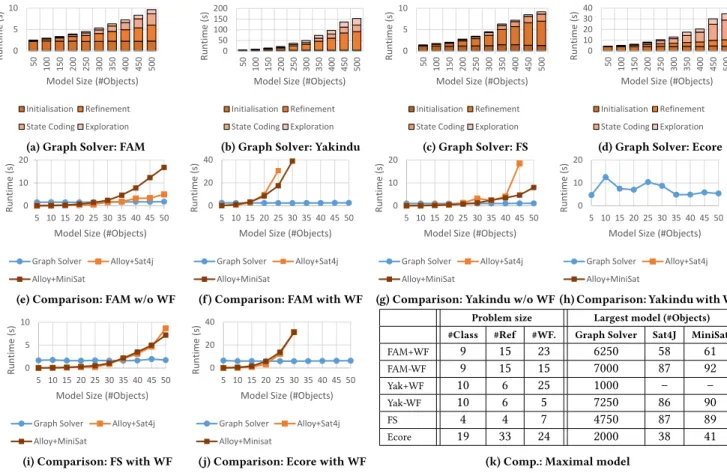
Experimental results.ForRQ1we evaluate the execution time of our approach for the four domains by increasing the target model size from 50 to 500 objects (with a step size of 50 new objects), and measuring (in Figure 8a–Figure 8d) the total execution time. As a key observation, our approach is able to generate consistent models with 500 elements for all four domains within 10 seconds for FAM and FS, within 40 seconds for Ecore and 3 minutes for Yakindu. As a stress test, we also managed to generate even larger consistent models (1000 objects for Yakindu, 7000 objects for FAM, 4750 objects for FS and 2000 objects for Ecore, see Figure 8k) in 20 minutes (as a median of 10 measurements).

ForRQ2, we compare model generation time of our Graph Solver with Alloy for small model sizes (from 5 to 50 objects, step size of 5 new objects) for the 6 test cases. As a baseline, we use a state-of-the- art EMF-to-Alloy mapping technique [16, 19, 24, 46, 47] and tool to obtain Alloy specifications for the Yakindu, FAM and Ecore domains, and the original Alloy specification is used for FS. According to the

1CPU: Intel Core-i5-m310M, MEM: 16GB, OS: Windows 10 Pro.

results (see Figure 8e–8j and Figure 8k), our approach scales much better as it generates models 1-2 orders of magnitude larger than Alloy could handle regardless of the back-end SAT solver which only had little impact on scalability. This is in line with previous measurements for Alloy in [19, 24]). Alloy dominantly ran out of memory when mapping input specification into a SAT problem which results in over 6 million variables and several million clauses when aiming to generate a model with 40-90 objects.

Note that the Alloy Analyzer is not primarily targeted to generate models but to check the consistency of a relational specification within a given scope and synthesize small counterexamples. In fact, Alloy had a smaller runtime for very small models, thus the warm-up cost of our graph solver is higher. However, our graph solver is able to generate much larger graph models even for all four domains with similar consistency guarantees as Alloy.

ForRQ3, we also measured (in Figure 8a–Figure 8d) how much time is spent in the different phases of model generation by our graph solver (see Figure 7) such as initialization, partial model refinement, state encoding and exploration. The preprocessing phase (1.5 seconds for FS, 4 seconds for Ecore, 2 seconds for FAM and 4 seconds for Yakindu) is a one-time penalty which is is proportional to the complexity of the metamodel and the WF constraints, thus we expect it to be negligible for model generation in case of other domains. Refinement is the dominant phase in the Yakindu and FS cases, while state encoding is dominant for Ecore. These results show that future research should primarily improve on refinement by providing a better transformation engine or refinement rules.

Quality of generated models.The quality of the generated models can be investigated from different aspects. To ensurecor- rectness, all WF constraints were checked on each generated graph instance by using an external tool, the VIATRA graph query engine [50]. To assessdiversitywhen a sequence of models are generated by the proposed graph solver (within similar scope), each model is guaranteed to be non-isomorphic by the state codes (Step(4)in Figure 7) or by a distance metric [51] in case of repeated calls to the solver, which offers increased diversity compared to Alloy [51].

Systematically assessing therealisticnature of models is a more complex task [13] which necessitates to obtain a large set of real models authored by engineers. Our graph solver ensures that only enumeration values can be isolated nodes in a graph otherwise all graphs are connected by default, i.e. all regular nodes are arranged into a containment hierarchy. In order to assure connectedness, Alloy requires an extra constraint to capture this concept, thus by default, our solution appears to be more realistic. In addition, [11, 13] contain an in-depth investigation of realistic models for the Yakindu domain. All generated models are available at [52].

Threats to validity.In order to strengtheninternal validity, our experiments include an extensive warm-up phase prior to the actual measurements to decrease the fluctuation of runtime results caused by the JVM (instead of the natural fluctuation of solver runtimes).

We used default setups for running Alloy and our graph solver, i.e.

no extra hints and performance optimizations were provided in the two approaches. Domain-specific fine tunings may improve scalability in some cases but it would simultaneously decrease the general-purpose nature of these solvers.

To addressexternal validity, our measurements cover 6 test cases including 3 industrial domains (Ecore, Yakindu, FAM) withcomplex

(9)

0 5 10

50 100 150 200 250 300 350 400 450 500

Runtime (s)

Model Size (#Objects)

Initialisation Refinement State Coding Exploration (a) Graph Solver: FAM

0 50 100 150 200

50 100 150 200 250 300 350 400 450 500

Runtime (s)

Initialisation Refinement State Coding Exploration (b) Graph Solver: Yakindu

0 5 10

50 100 150 200 250 300 350 400 450 500

Runtime (s)

Initialisation Refinement State Coding Exploration (c) Graph Solver: FS

0 10 20 30 40

50 100 150 200 250 300 350 400 450 500

Runtime (s)

Initialisation Refinement State Coding Exploration (d) Graph Solver: Ecore

0 10 20

5 10 15 20 25 30 35 40 45 50

Runtime (s)

Graph Solver Alloy+Sat4j Alloy+MiniSat

(e) Comparison: FAM w/o WF 0 20 40

5 10 15 20 25 30 35 40 45 50

Runtime (s)

(f) Comparison: FAM with WF 0 10 20

5 10 15 20 25 30 35 40 45 50

Runtime (s)

(g) Comparison: Yakindu w/o WF 0 10 20

5 10 15 20 25 30 35 40 45 50

Runtime (s)

(h) Comparison: Yakindu with WF

0 5 10

5 10 15 20 25 30 35 40 45 50

Runtime (s)

(i) Comparison: FS with WF 0 20 40

5 10 15 20 25 30 35 40 45 50

Runtime (s)

Graph Solver Alloy+Sat4j Alloy+Minisat

(j) Comparison: Ecore with WF

Problem size Largest model (#Objects)

#Class #Ref #WF. Graph Solver Sat4J MiniSat

FAM+WF 9 15 23 6250 58 61

FAM-WF 9 15 15 7000 87 92

Yak+WF 10 6 25 1000 – –

Yak-WF 10 6 5 7250 86 90

FS 4 4 7 4750 87 89

Ecore 19 33 24 2000 38 41

(k) Comp.: Maximal model Figure 8: Runtime comparison with increasing model size and distribution of generation time

structural WF constraints, thus our experimental scalability results for our graph solver are likely generalizable to other domains of similar size and complexity within the limitations of section 3.5. In case of simple WF constraints, the difference between the performance characteristics of Alloy and our graph solver may be smaller.

Since the performance of Alloy depends on the backend SAT-solver, our measurements already included two state-of-the-art solvers (SAT4J and MiniSAT). Thus the large scalability difference in the size of generated models can likely be attributed to our graph solver.

Summary.Our graph solver provides a strong platform for generating consistent graph models which are 1-2 orders of magnitude larger (with similar or higher quality) than derived by mapping based approaches using Alloy with an underlying SAT-solver. Such a difference in scalability can only partly be dedicated to our con- ceptually different approach which combines several advanced graph techniques to improve performance instead of fine-tuning a mapping. However, it likely indicates fundamental shortcomings of existing mapping based approaches. Based on in-depth profil- ing we suspect that representing each potential edge between a pair of nodes as a separate Boolean variable blows up the state space for sparse graph with only linear number of edges. Moreover, SAT-solvers have major problems in evaluating complex predicates over larger graph models [11] where graph query evaluation was particularly efficient [28].

Logic Uncertain Rule- Iterative Symbolic Solvers Models Based

Inputs

Partial Snapshot + ++ - + -

Local Constraints + - + + +

Global Constraints + - - + +

Outputs

Metamodel + + + + +

Well-formed + - - + +

Scalable - - ++ +/- -

Decidability - + + - +/-

Table 1: Comparison of related approaches

5 RELATED WORK

We compare our solution with existing model generation techniques with respect to the characteristics ofinputsandoutput resultsin Table 1. As forinputs, the model generation can be (1) initiated from apartial snapshot. Additionally, an approach may support (2) localand (3)global constraintsas WF constraints: a local constraint accesses only the attributes and the outgoing references of an object, while a global constraint specifies a complex structural pattern.

Local constraints are frequently attached to objects (e.g. in UML class diagrams), while global constraints are widely used in DSLs. As outputs, the generated models may (i) bemetamodel-compliant(ii) satisfy allwell-formednessconstraints of the language. We consider a technique (iv)scalableif there is no hard limit on the model size (as demonstrated in the respective papers). Finally, a model generation

(10)

approach may be (v)decidablewhich always terminates with a result. Our comparison excludes approaches like which do not guarantee metamodel- compliance of generated instance models.

Logic Solver Approaches.Several approaches map a model generation problem into a logic problem, which is solved by underlying SAT/SMT-solvers. Complete frameworks with standalone specification languages include Formula [35] (which uses Z3 SMT- solver [23]), Alloy [36] (which relies on SAT solvers like Sat4j[53]) and Clafer [20] (using backend reasoners like Alloy).

There are several approaches aiming to validate standardized engineering models enriched with OCL constraints [54] by relying upon different back-end logic-based approaches such as constraint logic programming [17, 37, 55], SAT-based model finders (like Alloy) [14, 16, 19, 24, 46, 47, 56], CSP solvers [49] first-order logic [57], constructive query containment [58], higher-order logic [59, 60], or rewriting logics [61]. Partial snapshots and WF constraints can be uniformly represented as constraints [19]. Growing models are supported in [15, 24] for a limited set of constraints.

Scalability of all these approaches are limited to small models / counter-examples. Furthermore, these approaches are either a priori bounded (where the search space needs to be restricted explicitly) or they have decidability issues. As our approach is independent from the actual mapping of constraints to logic formulae, it could potentially be integrated with most of the above techniques by complementing or replacing the back-end solvers.

Uncertain Models.Partial models are similar to uncertain models, which offer a rich specification language [38, 62] amenable to analysis. They a more user-friendly language compared to 3-valued interpretations, but without handling additional WF constraints.

Potential concrete models compliant with an uncertain model can be synthesized by the Alloy Analyzer [63], or refined by graph transformation rules [26]. Each concrete model is derived in a single step, thus their approach is not iterative like ours. Scalability analysis is omitted from these papers, but refinement of uncertain models is always decidable, thus termination is guaranteed.

Approaches like [64] analyze possible matches and executions of model transformation rules on partial models by using a SAT solver (MathSAT4) or by automated graph approximation (referred to as

“lifting”), or by graph query engines with [27]. As a key difference, our approach carries out model refinement while simultaneously evaluating graph query evaluation in an automated process.

Rule-based Instance Generators.A different class of model generators relies on rule-based synthesis driven by randomized, statistical or metamodel coverage information for testing purposes [65–67]. Some approaches support the calculation of effective metamodels [68], but partial snapshots are excluded from input specifications. Moreover, WF constraints are restricted to local constraints evaluated on individual objects while global constraints of a DSL are not supported. On the positive side, these approaches guarantee the diversity of models and scale well in practice [67, 69].

Iterative Approaches.Iterative approaches generate models by multiple solver calls. In [24] models are generated in by calling Alloy in multiple steps, where each step extends the instance model by a few elements. This approach scaled up to 50 object in 45s for generating valid Yakindu Statecharts. An iterative approach is pro- posedspecifically for allocation problemsin [70] based on Formula.

Models are generated in two steps to increase diversity of results

by first creating non-isomorphic submodels from an effective metamodel fragment followed by a problem-specific symmetry-breaking predicate [71] to ensures that no isomorphic models are generated twice while constraint checks are postponed to the very final stage.

An iterative, counter-example guided synthesis is proposed for higher-order logic formulae in [22], but the size of derived models is fixed and smaller than 50 objects.

Symbolic Model Generation TechniqueCertain techniques use abstract (or symbolic) graphs for analysis purposes. A tableau- based reasoning method is proposed for graph properties [72–74], which automatically refine solutions based on well-formedness constraints, and handle state space in the form of a resolution tree.

As a key difference, our approach refines possible solutions in the form of partial models, while [72, 73] resolves the graph constraints to a concrete solution. Therefore our approach is able to exploit efficient graph query engines to evaluate partial solutions, while those techniques are demonstrated on small (<10 objects) graphs or with no scalability evaluation at all.

Additionally, different approaches use abstract interpretation [29, 30], or predicate abstraction [31] for partial modeling. In those approaches, concretization is used to materialize (typically small) counter-examples for designated safety properties in a graph transformation system. However, their focus is to support model checking of abstract graph transformation systems, which can evaluate complex trajectories, but do not scale in the size of the models.

6 CONCLUSION AND FUTURE WORK

We presented a novel graph solver to generate consistent models of a designated size from a specification defined by a metamodel and a set of WF constraints. Unlike existing approaches which map the model generation problem to logic solvers (dominantly SAT or SMT-solvers), we address the model generation problem of consistent instances directly over graphs by combining advanced graph-based techniques with core SAT-solving rules. Our approach is fully automated and available as an open source tool [52].

Our experimental evaluation carried out over three industrial domains confirmed that our solver is able to synthesize consistent graph models with over 500-6000 objects with similar quality guarantees as provided by the popular relational model finder Alloy. The scalability of our solver is 1-2 orders of magnitude better than existing mapping based approaches using Alloy with a SAT-solver in the background. Such a difference in scalability likely indicates not only the benefits of our approach but also the inherent problems of mapping based model generation approaches deriving and solving a SAT problem. Thus our solver can serve as the output of map- pings that previously used Alloy for model generation purposes.

Altogether, our technique has the potential to be used in many testing scenarios including validation of large industrial DSLs, but its scalability is not yet sufficient for benchmarking purposes.

We have no precise claims on the diversity and realistic nature of our model generator. In the future, we aim to extend the framework to synthesize a set of graph models which are consistent, diverse and realistic at the same time. Numerous studies [24, 25, 51]

have demonstrated that neither traditional SAT-solvers nor SMT- solvers provide sufficient diversity for their outcome when called repeatedly.