Robust Classification Combined with Robust out-of-Distribution Detection: An Empirical
Analysis
Istv´an Megyeri University of Szeged
Szeged, Hungary imegyeri@inf.u-szeged.hu
Istv´an Heged ˝us University of Szeged
Szeged, Hungary ihegedus@inf.u-szeged.hu
M´ark Jelasity University of Szeged MTA-SZTE Research Group on AI
Szeged, Hungary jelasity@inf.u-szeged.hu
Abstract—Recently, out-of-distribution (OOD) detection has received considerable attention, because confident labels assigned to OOD examples represent a vulnerability similar to adversarial input perturbation. We are interested in models that combine the benefits of being robust to adversarial input and being able to detect OOD examples. Furthermore, we require that both in-distribution classification and OOD detection be robust to adversarial input perturbation. Several related studies apply an ad-hoc combination of several design choices to achieve similar goals. One can use several functions over the logit or soft-max layer for defining training objectives, OOD detection methods and adversarial attacks. Here, we present a design-space that covers such design choices, as well as a principled way of evaluating the networks. This includes a strong attack scenario where both in-distribution and OOD examples are adversarially perturbed to mislead OOD detection. We draw several interesting conclusions based on our empirical analysis of this design space.
Most importantly, we argue that the key factor is not the OOD training or detection method in itself, but rather the application of matching detection and training methods.
I. INTRODUCTION
Although computer vision models have achieved remarkable performance on various recognition tasks in recent years, they are susceptible to adversarial input [1]–[3], where invisibly small but well designed input perturbations mislead state- of-the-art models. The sensitivity of the current models to adversarial input indicates that these models are not aligned well with human perception. Among the many defenses against input perturbation, adversarial training has been found to be the most effective [4], [5]. In a nutshell, adversarial training means that the model is trained over the adversarially perturbed version of the training data to improve the robustness of the model.
Recently, robust out-of-distribution (OOD) detection also received considerable attention [6]–[8]. Adversarially trained models are relatively robust to adversarial input but they might assign high confidence to OOD samples. In a real-world application, this also represents a serious vulnerability [8].
Besides, OOD input is also open to adversarial perturbation,
Published in Proc. IJCNN 2021. DOI:10.1109/IJCNN52387.2021.9533635.
©2021 IEEE. This research was supported by the Ministry of Innovation and Technology NRDI Office within the framework of the Artificial Intelligence National Laboratory Program and the Artificial Intelligence National Excel- lence Program (grant 2018-1.2.1-NKP-2018-00008), as well as grant NKFIH- 1279-2/2020.
making OOD detection even harder. Recently, adversarial training on both in-distribution and OOD samples was shown to be able to increase the robustness of OOD detection [7], [8]. However, the proposed algorithms are somewhat ad-hoc, as the underlying design-space for robust training, detection, and attack methods has not been explicitly formalized and explored.
Here, we present a systematic design-space that covers most of the popular design choices for the various components. This includes the possible adversarial training objectives, robust OOD detection methods and adversarial attacks on both in- distributions and OOD samples. This allows us to propose ideal combinations of training and detection methods, and to explore the robustness to the various adversarial attacks.
We draw several interesting conclusions based on our empir- ical results. Most importantly, we argue that the key factor is not the OOD training or detection method in itself, but rather the application of matching detection and training methods.
This observation is important especially when both the in- distribution and OOD samples are adversarially perturbed.
This strong attack scenario has not been explored in related work yet. Also, it is interesting to note that among the detection methods that we evaluate here, the widely used Maximum Softmax Probability [9] baseline performed the poorest.
Our contributions can be summarized as follows:
• We identify the main components that can be used to systematically build training objectives, OOD detectors and attack methods that cover most algorithms from related work
• We experimentally analyze this design-space and we make a number of novel observations regarding the best combinations of these components
• We propose an evaluation methodology for measuring the robustness of the models under thestrongest possible attack, where we measure the robust accuracy over the in- distribution samples attacked based on the loss function, and the robust OOD detection performance after attacking both in-distribution and OOD samples based on the score function used by the OOD detector
II. RELATED WORK
Outlier, or OOD detection has long been a topic of inter- est [9]–[12]. Here, we focus on works where robustness to adversarial perturbation is a goal as well. Augustin et al. [7]
and Sehwag et al. [8] consider the problem of combining robust classification and robust OOD detection, like we do.
Sehwag et al. investigated the robustness of multiple OOD detection methods and found that existing OOD detectors are not robust. They proposed the adversarial training of a classifier, in which the OOD samples are considered an extra class. Augustin et al. used a different detection method for OOD samples. They require that the classifier outputs a uniform class distribution on perturbed OOD samples. Our contribution relative to these works is showing that training and detection have to be based on the same criteria in order to get the best performance, as well as proposing a principled evaluation method.
A number of studies make the assumption that adversarially perturbed in-distribution samples and OOD samples (such as noise, for example) should be treated in a similar fashion.
In effect, these approaches wish to characterize clean in- distribution samples. Hein et al. [6] attempt to reduce OOD confidence via using an adversarial training objective only for the OOD samples and show that this improves the detection of adversarial in-distribution samples as well. Stutz et al. [13]
propose to train the model to predict a uniform distribution for adversarial input and the correct class for clean input and show that this approach improves the detection of OOD samples as well. Lee et al. [14] assume that a pre-trained classifier is given. They wish to detect non-clean examples based on the softmax distribution of this classifier. Here, we assume that adversarially perturbed in-distribution samples must be assigned the correct label of their clean version. This is a significantly harder requirement.
One can also think of our work as an improvement of adversarial training [5] with a more realistic, stronger threat model. Indeed, although not in the focus of the present study, our extended adversarial training approach does improve adversarial accuracy relative to the work of Madry at al. [5].
Maini et al. [15] also extend adversarial training, but instead of using perturbed OOD samples, they apply a set of different perturbations over the in-distribution samples. Stutz et al. [13]
showed, however, that the approach of Maini et al. does not make models robust to attacked OOD samples. Combining these two different ways of extending adversarial training could be a direction for future work.
III. COMBINING OURTWOOBJECTIVES
We have two objectives that we want to achieve simulta- neously: robust classification and robust OOD detection. This raises a number of design issues. First of all, one has to design the model is such a way so as to support both classification and OOD detection at the same time. This can be done in many different ways. For example, in feed forward neural networks, we need to decide whether to base OOD detection on the logit layer or on the softmax layer, or whether to extend the classifier with an extra class representing OOD samples or not. Second, we need to define a combined loss function
that represents both objectives. This function will likely be different for OOD samples and normal samples.
In this section, we first present a framework in which these decisions can be represented. We then analyze related work and show how the main different design choices fit into this framework. This analysis will reveal that in related work the design decisions are often ad hoc in the sense that the OOD detection method and the training process are inconsistent, resulting in a suboptimal performance overall. When using our framework, the appropriate pairing of the training and detection method is evident.
A. Training Objectives
Let us first introduce some basic notations. We are inter- ested in the supervised classification task where each training example x ∈ Rd is drawn from an underlying theoretical distributionDin(that is,x∼ Din). SetCcontains the possible labels, and exactly one labely∈ Cis assigned to each training example in the training dataset. LetK=|C|denote the number of classes. Since the label is assumed to be a deterministic function of the example, we will also abuse the notation and write(x, y)∼ Din to indicate the label.
We are also given a set of unlabeled examples drawn from a distribution Dout over Rd such that Dout and Din are sufficiently different. From the point of view of the present study, a rigorous mathematical specification of the difference is not necessary. Instead, the key property ofDoutthat we rely on is that the probability of an examplexˆ ∼ Dout having a correct label withinC is vanishingly small.
Let the functionfθ:Rd→RK denote the output of a feed forward neural network classifier with parameters θ without the softmax normalization layer. In other words, fθ returns the so-called logit layer.
Robust classification can be formalized as a robust optimiza- tion problem [5]. Here, we are given a set of possible input perturbations, for example, ∆ ={δ : ||δ||∞ ≤ ǫ}. We want to minimize the loss of our classifier, assuming that the input can be perturbed using any perturbation from ∆, that is, we wish to solve the minimization problemminθρin(θ), where
ρin(θ) =E(x,y)∼Din[max
δ∈∆L(ey, fθ(x+δ))]. (1) Here,L(ey, fθ(x+δ))is a loss function of example(x, y)and model parametersθ, andeyis a one-hot encoded vector of the label y. From now on, we will assume that the loss function is the categorical cross-entropy function
L(y, f(x)) =− XK
i=1
yilogσ(f(x))i (2) although any differentiable loss function could be used. Here, function σ represents the softmax function, that is, σ(y)i = eyi/PK
j=1eyj.
The second objective is robustly detecting OOD samples fromDout. This needs a different loss function that is defined for the OOD training examples. Let us define ascore function s(fθ(x)), such that we expect a low score for OOD samples and a high score for in-distribution input. The score function is defined over the logit layer output, that is, we have s :
RK→R. Based on this score, we can define the OOD training objective to beminθρout(θ), where
ρout(θ) =Ex∼Dout[max
δ∈∆s(fθ(x+δ))] (3) When training the model on in-distribution and OOD samples simultaneously, the two optimization problems are combined as
minθ ρin(θ) +λρout(θ) (4) where λ is a weight parameter that controls the weight of in-distribution and OOD training examples.
B. Score Functions for OOD Detection
Now, let us turn to the OOD detection method. In our framework, it is a natural choice to use the score function for detection as well (not only training). This can be done via a suitable threshold that is supposed to separate OOD inputs from in-distribution inputs. Since the score function was part of the training objective, we can reasonably expect that the OOD examples will have a relatively low score. A suitable threshold exists if the in-distribution examples are expected to have a high score.
Our key observation is that for the existence of a suitable threshold, a necessary condition is that the score function has to be closely related to the loss function used to train over OOD samples.We now look at examples of training and detection methods from related work, and show whether or not these are suitably matched, in the light of this observation.
C. Training Objectives in Related Work
In this section, we discuss two common approaches to train models for OOD detection. In the first approach, the goal is to make the model output a uniform distribution when an OOD input is presented [7], [10]. This is implemented using the cross-entropy loss function with the uniform distribution as the true distribution:
ρuniout(θ) =Ex∼Dout[max
δ∈∆L(1/K, fθ(x+δ))] (5) In [6], instead of the distance from the uniform distribution, the maximum softmax probability was minimized for OOD samples. In this case, the optimum is the same, namely the maximal probability is minimized by the uniform distribution.
We can fit this approach into our framework if we chose the score function suni(x) =L(1/K, x). This would suggest, as discussed in Section III-B, that the model trained this way should use suni also for the detection of OOD examples.
Interestingly enough, that practice is not always followed in related work. For example, in both [7] and [10], the detection is implemented using smsp (see Section III-D), although Hendrycks et al. mention in the Appendix that suni might be more promising [10].
The second common representation is interpreting OOD samples as an extra background class [8], [16]. In this ap- proach, the objective is simply given by
ρlseout(θ) =Ex∼Dout[max
δ∈∆L(eK+1, fθ(x+δ))] (6) We propose a version of this approach, where we do not train extra parameters for the background class. Instead, we simply
append a constant to the logit layer of the model. As a result of training, the original classes from 1 toK can adapt to this constant so that this constant is maximal when the input is OOD. This way, the number of parameters will be the same as in the case of usingρuniout in (5), allowing for a fair comparison between the two approaches. In our experiments, we set this constant to zero, that is,fθ(x)K+1 = 0.
Now, let us examine how this approach fits into our frame- work. We have, using equation (2),
L(eK+1, fθ(x)) = log
K+1X
j=1
efθ(x)j. (7) This indicates that in this framework we can choseslse(x) = logPK+1
j=1 exj. This formula, called the LogSumExp (LSE) function, is known to be a smooth approximation of the maximum, and it was also proposed in [11] as the classifier energy function. Since fθ(x)K+1 is a constant, this function is a monotonous function of the LSE of the in-distribution classes (that is, the classes up to K). This indicates that in fact the decisive factor is whether the in-distribution classes have a small logit value, as opposed to the extra background class (the(K+ 1)th class) having the maximal value.
Again, this would suggest that the model trained this way should use slse (with an appropriate threshold) for the detection of OOD examples. Again, in related work this is not always the case. For example, Sehwag et al. [8] use the criteria whether the background class is maximal or not. Also, they do not useslseto attack OOD samples for testing robust OOD detection either, another natural choice that we will discuss in the following sections.
As a last note, the two approaches above (ρuniout and ρlseout) are far from being equivalent. The objective represented by ρlseout represents a larger degree of freedom, because the score function is applied before softmax normalization and because the uniform distribution is not enforced.
D. Score Function Summary
We list four score functions. The first two use the softmax normalized output and the remaining two use the logit values directly. A common baseline method is the maximum softmax probability (MSP) proposed in [9]:
smsp(fθ(x)) =kσ(fθ(x))k∞. (8) The score functionsuniwas proposed in [10]. These two score functions are based on the softmax output. Another possible score function is
sml(fθ(x)) =kfθ(x))k∞, (9) that is, the maximum logit. Although sml has not yet been used in related work, we include this variant in our evaluation because of its similarity tosmsp. The smooth version of this score function isslse, proposed in [11].
In the following, we will show experimentally that it is always advisable to use the score function for detecting OOD samples that is most similar to the training objectiveρout.
IV. EXPERIMENTAL SETUP
We are interested in the effect of the possible combinations of the various training objectives and score functions that we described previously, as well as the effect of other hyper- parameters such as the choice ofDoutand network capacity. In order to understand this, we performed a systematic empirical study, in which we combined training objectives and score functions, and used various hyper-parameters and databases for in-distribution and OOD samples. The two databases we used to represent in-distribution samples were MNIST [17]
and CIFAR-10 [18].
We first describe those settings that were common to the MNIST and CIFAR-10 experiments in Sections IV-A and IV-B. We then lay out the settings specific to the MNIST and CIFAR-10 experiments in Sections IV-C and IV-D, re- spectively.
We shall apply the PGD algorithm [19] in many different contexts. Let us introduce the notation PGDab, where the superscript a denotes the number of iterations and subscript b denotes the number of restarts. We omit the subscript when there is only one run.
A. Training
For preprocessing, we divided all the input values by 255, thus scaling the data into the range[0,1]d.
In each setting, we used adversarial training [5] for both in- distribution and OOD samples. The adversary during training was PGD (with database specific parameters defined later) that used the loss function in ρin for in-distribution samples, and the score function inρout for OOD samples, respectively. We held out1000 in-distribution samples as a validation set. We then selected the best model that was found during training according to the robust accuracy over the validation set, that is, the accuracy over the adversarially perturbed validation samples, as suggested in [20]. The validation samples were attacked using the same adversary as used for training in the case of CIFAR-10. For MNIST, we used a stronger adversary (PGD1005 ) because the training adversary (to be described below) was not able to reliably identify a unique maximum validation accuracy.
Throughout our evaluation, the training was performed with a batch size of 100, that consisted of50 in-distribution examples and50OOD examples. For the baseline case when no OOD samples were used, the batch size was 50.
Let us now describe the training objectives that we evalu- ated. The generic formula for the training objective is given in equation (4). This formula contains parameterλthat controls the relative weight of the in-distribution and OOD objective.
We evaluated three possible values of λ: 0.1,0.5, and 1.0.
λ = 0.1 means that the OOD samples will have the same contribution as any other in-distribution class (recall that each dataset defines 10 classes), essentially treating the OOD sam- ples as a 11th class. Sehwag et al. [8] applied this weighting strategy. λ= 1.0 means the distributionsDin andDout have equal importance. Hein et al. used this setting [6].
Apart from parameterλ, we also varied the OOD objective ρout. In particular, we experimented with two possible OOD objectives presented in equations (5) and (6). In total, the three values of λ and the two possible OOD objectives result in
6 = 3·2trainings for every combination of dataset and network architecture (to be described below).
B. Evaluation
We are interested in robust accuracy and robust OOD detection. Robust accuracy was measured as the accuracy against an untargeted PGD adversary [5]. In the attack, PGD maximized the loss used inρin. The performance of the non- robust OOD detection was measured using the area under curve (AUC) metric, as usual in related work (for exam- ple, [6], [7]). AUC is equal to the probability that a randomly chosen in-distribution sample x ∼ Din gets a larger score than a randomly chosen OOD sample xˆ ∼ Dout. That is, AUC=P(s(fθ(ˆx))≤s(fθ(x))). If the AUC is close to one then there exists a threshold that separates the OOD samples well. If the AUC is close to1/2then separation is not possible.
Since AUC is sensitive to imbalanced classes, it was calcu- lated using an equal number of samples from Din andDout. More precisely, we used1000samples from both distributions for each evaluation.
The robust version of OOD detection was evaluated by measuring the AUC after attacking only the OOD samples, or both the in-distribution and OOD samples. We note that in related work the hardest case, when both kinds of samples are attacked, has not yet been considered. In this robust version, the in-distribution samples are attacked using PGD minimizing the score of a given score function. In the case of the OOD samples, the same score function was maximized by PGD.
During the evaluation of robust OOD detection, we com- bined the 4 functions described in Section III-D, using them for both the attack and the detection method. These represent 4·4 = 16 possible attack-detection combinations.
C. MNIST-Specific Settings
a) Architecture: We trained the same convolutional net- work that was used in [5]. It has two convolutional layers and two dense layers with 32 and 64 filters, respectively. This is followed by a 2x2 max-pooling layer and a fully connected layer of 1024 neurons. ReLu activation was used.
b) Training: We used Adam [21] as our optimizer with a learning rate of10−4. We ran it for100epochs. The adversary during adversarial training was P GD40 with a step size of α= 10−2andǫ= 0.3. Recall, thatǫdefines the set of possible input perturbations:∆ ={δ:||δ||∞≤ǫ}.
We used two OOD datasets for training. The first one is the synthetic noise distribution introduced in [6], we will refer to it as DoutSN. In a nutshell, half of the inputs are generated uniformly at random and the other half is generated by permuting the pixels of images from the training set.
A Gaussian smoothing filter is applied for all the images, followed by a global rescaling into[0,1]d. The idea here is to preserve as much as possible from the global statistics of the original images while destroying the more complex features.
The second OOD dataset was the KMNIST dataset [22].
c) Evaluation: For the evaluation of OOD detection, we used the test sets of the two OOD datasets used for training and two additional datasets to test how OOD detection generalizes to unseen distributions. The first was the Fashion-MNIST [23]
test set and the second was uniform noise within [0,1]d, we
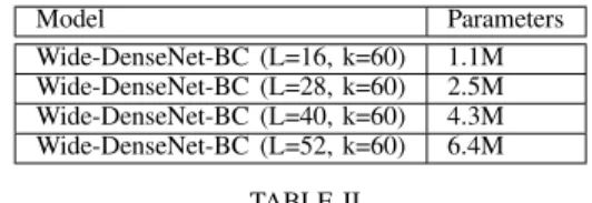
TABLE I
DENSENET[24]ARCHITECTURES USED FORCIFAR-10EXPERIMENTS.
Model Parameters
Wide-DenseNet-BC (L=16, k=60) 1.1M Wide-DenseNet-BC (L=28, k=60) 2.5M Wide-DenseNet-BC (L=40, k=60) 4.3M Wide-DenseNet-BC (L=52, k=60) 6.4M
TABLE II
ROBUST VALIDATION ACCURACY,CLEAN TEST ACCURACY,AND ROBUST TEST ACCURACY FORMNISTEXPERIMENTS
objective(ρout) Dout λ rob.val.acc. acc. rob.acc.
None 0.932 0.9895 0.9241
lse SN 0.1 0.935 0.9893 0.9277
lse K-MNIST 0.1 0.928 0.9897 0.9141
uni SN 1.0 0.93 0.9904 0.9144
uni K-MNIST 0.1 0.928 0.9887 0.9184
will refer to it as DoutU . PGD10050 was used for all the attacks (as in in [5]) with a step size ofα= 10−2andǫ= 0.3, except for Fashion-MNIST where we used ǫ= 0.1.
D. CIFAR-10-Specific Settings
a) Architecture: We used several wide variants of DenseNet [24], with the parameters listed in Table I. Thus, in this case, we performed our evaluation not only on a single network but on a range of networks with varying numbers of parameters. This allows us to examine the effect of network size.
b) Training: The optimizer we used was SGD with momentum 0.9 and an initial learning rate of 10−1. We ran this optimizer for 240epochs. The learning rate was divided by10at50%and75%of the training, as was done in [24]. In addition, we applied weight decay with a coefficient of10−4. We also applied standard augmentation: mirroring and shifting similarly to [5].
As adversary we used P GD10 with a step size of α = 2/255and withǫ= 8/255. Similarly to MNIST, we used two OOD datasets for training. Again, the first one is the synthetic noise distribution DSNout introduced in [6]. The second OOD dataset was the 80 Million Tiny Images dataset [25], we will refer to it asDoutT . This dataset was used also in [10] and [7].
This is a good choice because the global statistics and the low-level features of the images are similar to those of the CIFAR-10 images, while the high-level features are different.
This means that OOD detection is forced to focus on high-level features, which in turn increases its robustness to adversarial OOD inputs. Note that the CIFAR-10 dataset is actually a subset of the tiny images set, so we removed the CIFAR-10 classes like it was done in [10]. Afterwards, we separated a test set of 1000samples.
We note that the dataset in [6] performed very poorly here in our preliminary experiments so our experiments were run only for a single setting in this case, namely with the training objectiveρuniout andλ= 1.
c) Evaluation: For the evaluation of OOD detection, we used the test sets of the two OOD datasets used for training and two additional datasets to test how OOD detection generalizes to unseen distributions. The first was a set of 10,000 samples from the SVHN [26] test set. The second was uniform noise within [0,1]d. We will refer to it as DoutU . PGD2010 was used
0.8 0.81 0.82 0.83 0.84 0.85 0.86 0.87 0.88
16 28 40 52
accuracy
Network Depth (L)
0.44 0.46 0.48 0.5 0.52 0.54 0.56 0.58
16 28 40 52
robust accuracy
Network Depth (L) None
DoutSN +ρoutuni DoutT +ρoutuni DoutT +ρoutlse
Fig. 1. Clean test accuracy and robust test accuracy (PGD2010,ǫ= 8/255) on the CIFAR-10 dataset.
for all the attacks (as in in [5]) with a step size ofα= 2/255 and withǫ= 8/255.
V. RESULTS
We present our experimental results, organizing the discus- sion around our most important observations.
A. Robust Accuracy is not Reduced (MNIST) or Improved (CIFAR-10) by the OOD Adversarial Objective
Let us first focus on the accuracy of the in-distribution samples, with or without adversarial input perturbation. For the MNIST dataset, the results are included in Table II. When computing the robust accuracy, the samples were perturbed by PGD10050 , with ǫ = 0.3. The indicated λ values are the optimal choices among the possible choices ofλfor the given objective according to the robust accuracy on the validation set against aP GD1005 adversary. The value “None” indicates plain adversarial training without an OOD objective.
It is clear that adding the OOD objective does not reduce robust accuracy. We also note that our reported value of0.9241 is significantly higher than the one reported in [5]. This is because of our better early stopping criterion based on a stronger adversary used over the validation set.
Accuracy values for the CIFAR-10 dataset are shown in Figure 1. The OOD datasetsDSNout andDTout were described in Section IV-D. We show the results with the best choice of parameterλaccording to the robust accuracy on the validation set against aP GD10 adversary.
Robust accuracy is significantly improved compared to plain adversarial learning, while clear accuracy remains approxi- mately the same. It is also interesting to note that increasing
0.4 0.5 0.6 0.7 0.8 0.9 1
16 28 40 52
AUC
Network Depth (L) None Attacked
0.4 0.5 0.6 0.7 0.8 0.9 1
16 28 40 52
AUC
Network Depth (L) OOD Attacked
0.4 0.5 0.6 0.7 0.8 0.9 1
16 28 40 52
AUC
Network Depth (L) None
DoutSN +ρoutuni DoutT +ρoutuni DoutT +ρoutlse AUC = 1/2
IN+OOD Attacked
Fig. 2. OOD detection AUC over CIFAR-10 under three different kinds of attack scenarios: no attack, only OOD samples are perturbed and both in-distribution and OOD samples are perturbed.
NO NO NO LSE ML MSP UNI LSE ML MSP UNI LSE ML MSP UNI LSE ML MSP UNI LSE ML MSP UNI LSE ML MSP UNI
LSE ML MSP UNI
None uni lse
NoneNoneuniunilselse
NoneOOD attackedIN+OOD attackedAttacks & Models
Detection method
.97 .97 .96 .97
1 1 1 1
1 1 .99 .21
.77 .77 .75 .78
.77 .77 .75 .78
.81 .81 .70 .82
.78 .78 .76 .77
.99 .99 1 1
.99 .99 .99 1
.99 .99 .99 1
.99 .99 .99 1
1 1 .97 .19
1 1 .95 .35
1 1 .93 .35
1 1 .98 .09
.52 .52 .52 .54
.53 .52 .51 .54
.64 .64 .39 .66
.54 .54 .53 .52
.91 .95 .98 .99
.91 .95 .97 .99
.96 .97 .96 1
.93 .96 .98 .99
1 1 .95 .13
1 1 .90 .25
1 1 .84 .26
1 1 .96 .05
0 0.2 0.4 0.6 0.8 1
AUC
MNIST
NO NO NO LSE ML MSP UNI LSE ML MSP UNI LSE ML MSP UNI LSE ML MSP UNI LSE ML MSP UNI LSE ML MSP UNI
LSE ML MSP UNI LSE ML MSP UNI
16 52
None uni lse NoneNoneuniunilselse
NoneOOD attackedIN+OOD attackedAttacks & Models
Network Depth & Detection Method
.86 .88 .87 .86 .89 .90 .90 .89
.95 .94 .94 .95 .95 .95 .95 .95
.93 .94 .85 .84 .94 .95 .89 .89
.68 .70 .71 .68 .72 .73 .74 .72
.69 .69 .65 .69 .73 .73 .72 .73
.75 .72 .61 .75 .79 .77 .68 .79
.68 .70 .71 .68 .72 .73 .74 .72
.83 .81 .80 .83 .84 .84 .83 .84
.85 .81 .79 .85 .86 .84 .82 .86
.85 .81 .79 .85 .86 .84 .82 .86
.83 .81 .80 .83 .84 .84 .83 .84
.80 .81 .76 .75 .84 .85 .80 .80
.82 .80 .69 .74 .85 .84 .74 .79
.88 .85 .61 .74 .90 .88 .67 .79
.86 .85 .70 .66 .89 .88 .74 .73
.39 .42 .52 .39 .43 .45 .54 .43
.42 .41 .40 .42 .45 .45 .46 .45
.63 .53 .34 .63 .66 .60 .37 .66
.39 .42 .52 .39 .43 .45 .54 .43
.61 .61 .61 .61 .65 .65 .64 .65
.69 .60 .57 .69 .71 .64 .62 .71
.72 .62 .57 .72 .74 .66 .62 .74
.61 .61 .61 .61 .65 .65 .64 .65
.56 .58 .62 .56 .61 .65 .68 .63
.61 .57 .44 .55 .66 .63 .50 .61
.82 .73 .32 .61 .86 .77 .38 .67
.73 .70 .51 .38 .77 .73 .54 .45
0.2 0.3 0.4 0.5 0.6 0.7 0.8 0.9 1
AUC
CIFAR-10
Fig. 3. OOD detection AUC over MNIST and CIFAR-10 under three different kinds of attack scenarios: no attack, only OOD samples are perturbed, and both in-distribution and OOD samples are perturbed. These attacks are indicated on the vertical axis. Under each attack, the three different OOD training objectives are indicated: None,ρunioutandρlseout. Under each training objective, 4 different score functions are indicated that are used for attacking samples at detection time. The horizontal axis indicates possible score functions used for detection. The CIFAR-10 plot also includes the smallest and largest network architecture, indicated on the horizontal axis. During training,DoutSNwas used on MNIST, andDoutT on CIFAR-10.
the network size in general increases robust accuracy, a well- known fact that has been pointed out in [5] as well. The best choice is the uniform OOD objective with the Tiny Images OOD dataset in this case.
Similar observations were reported in [7] for an l2 threat model (here, we use thel∞norm, as described before). How- ever, our results highlight another important factor, namely the choice of the objective function. Although bothρuniout andρlseout improve the robust performance compared to plain adversarial training,ρuniout is a significantly better choice.
B. OOD Training Objective has Strongest Effect under Strongest Attack
Let us now look at how the OOD training objectives affect the ability of the models to detect OOD samples, under different kinds of adversarial attacks applied at detection time.
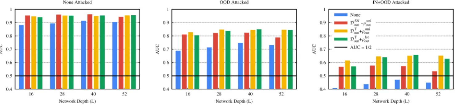
Figure 2 illustrates the effect of the three kinds of adversarial attacks: (1) no attack (clean inputs), (2) only the OOD inputs are attacked and (3) both in-distribution and OOD inputs are attacked.
The adversary wasP GD2010usingǫ= 8/255. The indicated AUC values are averages of AUC values computed over 13 test OOD databases, given by the 10 classes of the SVHN dataset (each treated as a separate OOD database) and the test sets of the databasesDTout,DoutSN andDUout. For a given OOD dataset
we calculated the AUC value as a minimax value: for all the 4 possible score functions used for detection we computed the minimum AUC value over the 4 possible score functions used for the attack. We then took the maximum of these values, which gives the minimax AUC.
What is clear is that for clean examples the training ob- jectives have a relatively little effect, although not using an OOD objective is consistently the worst option. The harder the attack the larger the relative difference becomes between the model that did not use any OOD objective during training and those that did. Here, the decisive factor appears to be the OOD database used during training:DToutseems to be the best choice.
The same conclusion is valid also in the case of the MNIST dataset. This is evident from Figure 3, where the OOD detection AUC values are illustrated in a finer resolution for both MNIST and CIFAR-10. Here, compared to Figure 2, the AUC values are not aggregated using the minimax technique but instead all the 4·4 = 16 combinations of detection and attacking score functions are included individually. The values are still averages over our test OOD datasets. For CIFAR-10 we used the same 13 sets described above. For MNIST, we used 22 datasets, given by 10 classes of Fasion-MNIST, 10 classes of K-MNIST, and the test sets ofDSNout andDUout.
LSE ML MSP UNI LSE ML MSP UNI LSE ML MSP UNI
0 1 2 3 4 5 6 7 8 9 0 1 2 3 4 5 6 7 8 9Dout UDout
SN
F-MNIST K-MNIST
NoneSNK-MNISTTraining OOD Datasets & Defenses
Test OOD Datasets
.37 .77 .64 .70 .76 .64 .54 .78 .74 .55 .45 .40 .53 .50 .41 .58 .47 .43 .49 .42 .31 .01 .37 .77 .65 .70 .76 .64 .55 .77 .74 .55 .45 .39 .53 .50 .41 .58 .47 .43 .49 .41 .31 .01 .41 .61 .56 .63 .70 .42 .49 .38 .61 .43 .29 .32 .36 .27 .30 .44 .36 .27 .34 .25 .19 0 .37 .84 .65 .75 .76 .59 .56 .65 .75 .57 .41 .43 .55 .44 .40 .57 .49 .42 .54 .40 .38 .01 .93 .94 .93 .93 .93 .87 .93 .89 .93 .93 .91 .89 .90 .90 .89 .90 .87 .91 .90 .90 .89 .85 .98 .97 .98 .97 .98 .89 .98 .90 .98 .97 .96 .91 .92 .96 .93 .92 .89 .95 .94 .94 .97 .95 .99 .98 1 .98 1 .87 1 .88 .99 .99 .98 .90 .91 .98 .93 .91 .87 .95 .95 .94 1 1 1 1 1 1 1 .98 1 .98 1 1 1 .98 .99 1 .99 .99 .97 .99 .99 .99 1 1 .86 .88 .88 .89 .90 .89 .88 .93 .89 .90 .87 .88 .88 .85 .87 .89 .88 .85 .87 .88 .54 .50 .96 .97 .97 .97 .98 .91 .97 .95 .97 .96 .97 .96 .97 .96 .96 .97 .96 .95 .96 .97 .83 .79 .99 1 .99 .99 1 .85 1 .92 .99 .97 .99 .99 .99 .99 .99 .99 .97 .99 .99 .99 1 1
1 1 1 1 1 .96 1 .99 1 .99 1 1 1 1 1 1 .99 1 1 1 1 1
0 0.2 0.4 0.6 0.8 1
Robust AUC
MNIST
LSE ML MSP UNI LSE ML MSP UNI LSE ML MSP UNI LSE ML MSP UNI LSE ML MSP UNI LSE ML MSP UNI
0 1 2 3 4 5 6 7 8 9
SVHN
Dout T Dout
SN Dout U 16
16 16
52 52 52
NoneSNTTraining OOD Datasets & Defenses
Test OOD Datasets
.38 .40 .39 .39 .41 .40 .39 .39 .36 .36 .33 .39 .47
.41 .44 .42 .42 .43 .42 .42 .41 .39 .39 .33 .42 .39
.37 .41 .35 .37 .37 .35 .37 .36 .34 .35 .25 .35 .18
.38 .40 .39 .39 .41 .40 .39 .39 .36 .36 .33 .39 .47
.48 .48 .43 .45 .46 .45 .47 .41 .44 .43 .33 .47 .25
.50 .51 .45 .48 .48 .47 .49 .42 .46 .46 .33 .50 .25
.41 .42 .37 .40 .38 .38 .42 .34 .39 .39 .25 .41 .27
.48 .48 .43 .45 .46 .45 .47 .41 .44 .43 .33 .47 .25
.54 .54 .58 .60 .57 .59 .55 .54 .54 .54 .30 .98 .38
.56 .57 .59 .62 .58 .60 .57 .54 .55 .56 .30 .98 .36
.48 .49 .50 .53 .49 .51 .48 .45 .47 .48 .22 .98 .21
.54 .54 .58 .60 .57 .59 .55 .54 .54 .54 .30 .98 .38
.52 .55 .55 .58 .54 .56 .52 .48 .49 .52 .29 .99 .25
.53 .56 .56 .59 .55 .56 .53 .48 .50 .53 .30 .99 .25
.40 .43 .42 .45 .40 .42 .41 .36 .37 .40 .22 .99 .24
.52 .55 .55 .58 .54 .56 .52 .48 .49 .52 .29 .99 .25
.65 .69 .57 .58 .54 .57 .59 .58 .57 .56 .60 .50 .98
.62 .66 .55 .57 .53 .55 .57 .55 .56 .55 .56 .51 .97
.59 .62 .52 .54 .50 .52 .54 .52 .53 .52 .53 .48 .96
.65 .69 .57 .58 .54 .57 .59 .58 .57 .56 .60 .50 .98
.69 .73 .61 .62 .57 .62 .62 .57 .62 .60 .68 .54 .98
.68 .71 .60 .61 .57 .61 .62 .56 .61 .60 .65 .56 .98
.64 .68 .57 .58 .54 .57 .59 .53 .58 .57 .63 .53 .98
.69 .73 .61 .62 .57 .62 .62 .57 .62 .60 .68 .54 .98
0 0.2 0.4 0.6 0.8 1
Robust AUC
CIFAR-10
Fig. 4. OOD detection AUC over MNIST and CIFAR-10 under combinations of OOD datasets used during training and detection. The databases used for training are indicated on the vertical axis. The training objectives were ρuniout in both cases. Under each training OOD dataset, 4 different score functions are indicated that are used for detection. The horizontal axis indicates OOD datasets used for evaluation. The CIFAR-10 plot also includes the smallest and largest network architecture, indicated on the vertical axis.
For MNIST as well, clearly, the harder the attack the larger the relative difference becomes between the models that did or did not use any OOD objective during training.
Let us point out here, that our strongest attack is signif- icantly stronger than the attacks normally studied in related work, where in-distribution samples are not perturbed during the OOD detection task. Also, as Figure 2 reveals, the AUC barely improves when increasing the size of the network. It is possible that improvements would appear only with much larger networks.
C. Attacks on OOD Samples are most Effective when Attack- ing and Detection Score Functions are the Same
Ideally, we want to use the strongest possible attack when testing the robustness of any machine learning model. How- ever, so far, it has not been clear how the strongest attack should be designed for a given OOD detection mechanism. In our framework based on score functions, it is rather natural to assume that maximizing the score function used for detection is the strongest attack.
This conclusion is supported by the data in Figure 3. As we, for all the detection methods, the minimal AUC value belongs to the attack method that uses the same score functions, in all the three attack scenarios, for all the training objectives, for both MNIST and CIFAR-10.
D. OOD Detection and OOD Training Objective should Use the same Score Function
In the framework based on score functions, we can examine the relationship between the training objective and the detec- tion method for OOD samples. A natural hypothesis is that these two components should be based on the same score function in order to enforce the best possible AUC value.
This conclusion can be verified in Figure 3. To see this, recall that we are interested in the minimax AUC value, that is, we want to maximize the minimal AUC value over the possible pairs of score functions used for OOD training and detection. In other words, we assume that the attacker knows
the detection method as well as the training method and so she can pick the attack resulting in the minimal AUC. In the table, for all pairs of training and detection score functions four attacks are listed. The minimum of these is always maximal when the training and detection score functions are the same.
E. The Learned Robust Models do not Generalize Well for Unseen OOD Datasets
It is a central question whether robust OOD detection generalizes beyond the OOD dataset that was used during the adversarial training. We will argue that, when taking a closer look, we can find a number of problems regarding this kind of generalization, which opens up novel research questions.
Note that we work with training objectives, OOD datasets and detection methods that are used in the state-of-the art approaches, but under a stronger threat model.
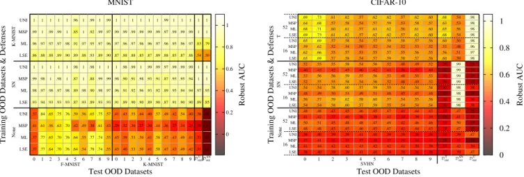
Figure 4 focuses on the generalization of OOD detection.
The values shown in the table correspond to those of the most successful attacks, that is, the table represents the worst case scenario. The most successful attack, as described previously, is the scenario when both in-distribution and OOD samples are adversarially perturbed, based on the same score function that is used for detection. The databases are examined at a fine resolution, that is, we consider all the classes of the unseen databases (see sections IV-C and IV-D) as a separate database.
We can see that the models do not generalize equally well to each OOD dataset. On MNIST, the models seem to be less effective in identifying some classes as OOD, for example, Fashion-MNIST classes 5 (Sandal) and 7 (Sneaker). Similar observations can be made regarding the CIFAR-10 models.
For example, SVHN classes 0 and 1 are identified as OOD much easier than the other classes.
We can also see that, overall, the DTout dataset offers the best robust OOD performance over CIFAR-10. However, it is remarkable that training withDToutdoes not generalize well to DSNout (although it does generalize to the uniform distribution DUout) and the performance is not very impressive on the test set of DTout either. On the other hand, training with DSNout is
radically different: in that case the model clearly overfitsDoutSN without any generalization toDTout orDUout. This suggests that a mixture of multiple OOD datasets might be a better choice for representing OOD samples during training.
VI. CONCLUSIONS
We defined a design space, where one can define training objectives, detection methods and attack methods for the com- bination of the robust OOD detection problem and the robust classification problem with the help of a set of score functions.
Also, we introduced a strong threat model in which both in- distribution and OOD samples are adversarially perturbed to mislead OOD detection.
We performed a thorough empirical evaluation of this framework. We found that adding an adversarial OOD objec- tive to the training method does not hurt robust in-distribution accuracy, in fact, a significant improvement can be seen in some cases. This indicates that it is always safe to add such an objective.
We also found that it is impossible to pick a score function for robust OOD detection independently of how the model in question was trained. Instead, we get the best results when training and detection is based on the same score function.
In other words, while non-robust OOD detection is more robust to the training procedure, in robust OOD detection it is more important to align the detection method with the training method, that is, to use the same score function in both. Also, a similar statement can be formulated in terms of the OOD detection method and the attack on this detection method. The most successful attack is performed using the same score function as the one used by the detection method.
We also pointed out that a deeper understanding of how OOD detectors generalize to unseen distributions is an inter- esting direction for future research.
REFERENCES
[1] Christian Szegedy, Wojciech Zaremba, Ilya Sutskever, Joan Bruna, Dumitru Erhan, Ian Goodfellow, and Rob Fergus. Intriguing properties of neural networks. InInt. Conf. on Learning Representations, 2014.
[2] Seyed-Mohsen Moosavi-Dezfooli, Alhussein Fawzi, and Pascal Frossard. Deepfool: A simple and accurate method to fool deep neural networks. InProc. of the IEEE Conf. on Computer Vision and Pattern Recognition (CVPR), June 2016.
[3] N. Carlini and D. Wagner. Towards evaluating the robustness of neural networks. In2017 IEEE Symp. on Security and Privacy (SP), pages 39–57, 2017.
[4] Ian J. Goodfellow and Jonathon Shlens Christian Szegedy. Explaining and harnessing adversarial examples. In 3rd Int. Conf. on Learning Representations (ICLR), 2015.
[5] Aleksander Madry, Aleksandar Makelov, Ludwig Schmidt, Dimitris Tsipras, and Adrian Vladu. Towards deep learning models resistant to adversarial attacks. InInt. Conf. on Learning Representations, 2018.
[6] Matthias Hein, Maksym Andriushchenko, and Julian Bitterwolf. Why relu networks yield high-confidence predictions far away from the training data and how to mitigate the problem. In IEEE Conf. on Computer Vision and Pattern Recognition, CVPR 2019, Long Beach, CA, USA, June 16-20, 2019, pages 41–50. Computer Vision Foundation / IEEE, 2019.
[7] Maximilian Augustin, Alexander Meinke, and Matthias Hein. Adver- sarial robustness on in- and out-distribution improves explainability. In Andrea Vedaldi, Horst Bischof, Thomas Brox, and Jan-Michael Frahm, editors,Computer Vision - ECCV 2020 - 16th European Conf., Glasgow, UK, August 23-28, 2020, Proc., Part XXVI, volume 12371 ofLecture Notes in Computer Science, pages 228–245. Springer, 2020.
[8] Vikash Sehwag, Arjun Nitin Bhagoji, Liwei Song, Chawin Sitawarin, Daniel Cullina, Mung Chiang, and Prateek Mittal. Analyzing the robustness of open-world machine learning. In Proc. of the 12th ACM Workshop on Artificial Intelligence and Security, AISec’19, page 105–116, New York, NY, USA, 2019. Association for Computing Machinery.
[9] Dan Hendrycks and Kevin Gimpel. A baseline for detecting misclassified and out-of-distribution examples in neural networks. In5th Int. Conf.
on Learning Representations, ICLR 2017, Toulon, France, April 24-26, 2017, Conf. Track Proc.OpenReview.net, 2017.
[10] Dan Hendrycks, Mantas Mazeika, and Thomas Dietterich. Deep anomaly detection with outlier exposure. In Int. Conf. on Learning Representations, 2019.
[11] Will Grathwohl, Kuan-Chieh Wang, Joern-Henrik Jacobsen, David Du- venaud, Mohammad Norouzi, and Kevin Swersky. Your classifier is secretly an energy based model and you should treat it like one. InInt.
Conf. on Learning Representations, 2020.
[12] Shiyu Liang, Yixuan Li, and R. Srikant. Enhancing the reliability of out-of-distribution image detection in neural networks. InInt. Conf. on Learning Representations, 2018.
[13] David Stutz, Matthias Hein, and Bernt Schiele. Confidence-calibrated adversarial training: Generalizing to unseen attacks. In Hal Daum´e III and Aarti Singh, editors, Proc. of the 37th Int. Conf. on Machine Learning, volume 119 ofProc. of Machine Learning Research, pages 9155–9166. PMLR, 13–18 Jul 2020.
[14] Kimin Lee, Kibok Lee, Honglak Lee, and Jinwoo Shin. A simple unified framework for detecting out-of-distribution samples and adversarial attacks. In S. Bengio, H. Wallach, H. Larochelle, K. Grauman, N. Cesa- Bianchi, and R. Garnett, editors, Advances in Neural Information Processing Systems, volume 31, pages 7167–7177. Curran Associates, Inc., 2018.
[15] Pratyush Maini, Eric Wong, and Zico Kolter. Adversarial robustness against the union of multiple perturbation models. In Hal Daum´e III and Aarti Singh, editors,Proc. of the 37th Int. Conf. on Machine Learning, volume 119 ofProc. of Machine Learning Research, pages 6640–6650.
PMLR, 13–18 Jul 2020.
[16] Michael McCoyd and David A. Wagner. Background class defense against adversarial examples. In 2018 IEEE Security and Privacy Workshops, SP Workshops 2018, San Francisco, CA, USA, May 24, 2018, pages 96–102. IEEE Computer Society, 2018.
[17] Yann Lecun, L´eon Bottou, Yoshua Bengio, and Patrick Haffner.
Gradient-based learning applied to document recognition. Proc. of the IEEE, 86(11):2278–2324, November 1998.
[18] Alex Krizhevsky, Geoffrey Hinton, et al. Learning multiple layers of features from tiny images. Technical report, Citeseer, 2009.
[19] Alexey Kurakin, Ian J. Goodfellow, and Samy Bengio. Adversarial machine learning at scale. In5th Int. Conf. on Learning Representations, ICLR, 2017.
[20] Leslie Rice, Eric Wong, and Zico Kolter. Overfitting in adversarially robust deep learning. In Hal Daum´e III and Aarti Singh, editors,Proc.
of the 37th Int. Conf. on Machine Learning, volume 119 ofProc. of Machine Learning Research, pages 8093–8104. PMLR, 13–18 Jul 2020.
[21] Diederik P. Kingma and Jimmy Ba. Adam: A method for stochastic optimization, 2014. cite arxiv:1412.6980Comment: Published as a Conf.
paper at the 3rd Int. Conf. for Learning Representations, San Diego, 2015.
[22] Tarin Clanuwat, Mikel Bober-Irizar, Asanobu Kitamoto, Alex Lamb, Kazuaki Yamamoto, and David Ha. Deep learning for classical Japanese literature. Technical Report cs.CV/1812.01718, arXiv, 2018.
[23] Han Xiao, Kashif Rasul, and Roland Vollgraf. Fashion-mnist: a novel image dataset for benchmarking machine learning algorithms. Technical Report cs.LG/1708.07747, arXiv, 2017.
[24] Gao Huang, Zhuang Liu, Laurens van der Maaten, and Kilian Q Weinberger. Densely connected convolutional networks. In Proc. of the IEEE Conf. on Computer Vision and Pattern Recognition, 2017.
[25] Antonio Torralba, Rob Fergus, and William T. Freeman. 80 million tiny images: A large data set for nonparametric object and scene recognition.
IEEE Trans. Pattern Anal. Mach. Intell., 30(11):1958–1970, November 2008.
[26] Yuval Netzer, Tao Wang, Adam Coates, Alessandro Bissacco, Bo Wu, and Andrew Y. Ng. Reading digits in natural images with unsupervised feature learning. InNIPS Workshop on Deep Learning and Unsupervised Feature Learning 2011, 2011.