Towards the Automated Generation of Consistent, Diverse, Scalable and Realistic Graph Models

Towards the Automated Generation of Consistent, Diverse, Scalable and Realistic

Graph Models

D´aniel Varr´o^1,2,3, Oszk´ar Semer´ath^1,2, G´abor Sz´arnyas^1,2, and Akos Horv´´ ath^1,4

1 Budapest University of Technology and Economics

2 MTA-BME Lend¨ulet Research Group on Cyber-Physical Systems

3 McGill University, Department of Electrical and Computer Engineering

4 IncQuery Labs Ltd.

{varro,semerath,szarnyas,ahorvath}@mit.bme.hu

Abstract. Automated model generation can be highly beneficial for var- ious application scenarios including software tool certification, validation of cyber-physical systems or benchmarking graph databases to avoid te- dious manual synthesis of models. In the paper, we present a long-term research challenge how to generate graph models specific to a domain which are consistent, diverse, scalable and realistic at the same time.

We provide foundations for a class of model generators along a refine- ment relation which operates over partial models with 3-valued repre- sentation and ensures that subsequently derived partial models preserve the truth evaluation of well-formedness constraints in the domain. We formally provecompleteness, i.e. any finite instance model of a domain can be generated by model generator transformations in finite steps and soundness, i.e. any instance model retrieved as a solution satisfies all well-formedness constraints. An experimental evaluation is carried out in the context of a statechart modeling tool to evaluate the trade-off between different characteristics of model generators.

Keywords: automated model generation, partial models, refinement

1 Introduction

Smart and safe cyber-physical systems [16, 54, 69, 93] are software-intensive au- tonomous systems that largely depend on the context in which they operate, and frequently rely upon intelligent algorithms to adapt to new contexts on-the-fly.

However, adaptive techniques are currently avoided in many safety-critical sys- tems due to major certification issues. Automated synthesis of prototypical test contexts [58] aims to systematically derive previously unanticipated contexts for assurance of such smart systems in the form of graph models. Such prototype contexts need to be consistent, i.e. they need to fulfill certain well-formedness (consistency) constraints when synthesizing large and realistic environments.

In many design and verification tools used for engineering CPSs, system models are frequently represented as typed and attributed graphs. There has been an increasing interest in model generators to be used for validating, testing or benchmarking design tools with advanced support for queries and transfor- mations [4, 6, 42, 92]. Qualification of design and verification tools is necessi- tated by safety standards (like DO-178C [89], or ISO 26262 [43]) in order to assure that their output results can be trusted in safety-critical applications.

However, tool qualification is extremely costly due to the lack of effective best practices for validating the design tools themselves. Additionally, design-space exploration [47,57,66] necessitates to automatically derive different solution can- didates which are optimal wrt. certain objectives for complex allocation prob- lems. For testing and DSE purposes,diversemodels need to be synthesized where any pairs of models are structurally very different from each other in order to achieve high coverage or a diverse solution space.

Outside the systems engineering domain, many performance benchmarks for advanced relational databases [26], triple stores and graph databases [13, 60, 80], or biochemical applications [36,99] also rely on the availability of extremely large andscalable generators of graph models.

Since real models created by engineers are frequently unavailable due to the protection of intellectual property rights, there is an increasing need ofrealistic models which have similar characteristics to real models. However, these models should be domain-specific, i.e. graphs of biomedical systems are expected to be very different from graphs of social networks or software models. An engineer can easily distinguish an auto-generated model from a manually designed model by inspecting key attributes (e.g. names), but the same task becomes more chal- lenging if we abstract from all attributes and inspect only the (typed) graph structure. While several graph metrics have been proposed [10, 12, 44, 68], the characterization ofrealistic models is a major challenge [91].

As a long-term research challenge, we aim at automatically generating domain- specific graph models which are simultaneously scalable, realistic, consistent and diverse. In the paper, we precisely formulate the model generation challenge for the first time (Section 2). Then in Section 3, we revisit the formal foundations of partial models and well-formedness constraints captured by graph patterns. In Section 4, we propose a refinement calculus for partial models as theoretical foun- dation for graph model generation, and a set of specific refinement operations as novel contributions. Moreover, we precisely formulate certain soundness and completeness properties of this refinement calculus.⁵ In addition, we carry out an experimental evaluation of some existing techniques and tools in Section 5 to assess the trade-off between different characteristics (e.g. diverse vs. realis- tic, consistent vs. diverse, diverse vs. consistent and consistent vs. scalable) of model generation. Finally, related work is discussed wrt. the different properties required for model generation in Section 6.

5 The authors’ copy of this paper is available athttps://inf.mit.bme.hu/research/

publications/towards-model-generation together with the proofs of theorems presented in Section 4.

2 The Graph Model Generation Challenge

A domain specification (or domain-specific language, DSL) is defined by ameta- model MM which captures the main concepts and relations in a domain, and specifies the basic graph structure of the models. In addition, a set of well- formedness constraints WF = {ϕ1, . . . , ϕn} may further restrict valid domain models by extra structural restrictions. Furthermore, we assume that editing operations of the domain are also defined by a set of rulesOP.

Informally, the automated model generation challenge is to derive a set of instance models where each M_i conforms to a metamodel MM. A model gen- erator Gen ↦→ {M_i} derives a set (or sequence) of models along a derivation sequenceM0

op1,...,opk

−−−−−−→Mi starting from (a potentially empty) initial modelM0

by applying some operationsopj fromOP at each step. Ideally, a single model M_i or a model generatorGenshould satisfy the following requirements:

– Consistent (CON): A modelM_i is consistent if it satisfies all constraints inWF (denoted byM_i |=WF). A model generatorGenis consistent, if it is sound (i.e. if a model is derivable then it is consistent) and complete (i.e.

all consistent models can be derived).

– Diverse (DIV): The diversity of a model M_i is defined as the number of (direct) types used from itsMM:M_i is more diverse thanM_j if more types of M M are used in M_i than in M_j. A model generator Gen is diverse if there is a designated distance between each pairs of models M_i and M_j: dist(M_i, M_j)> D.

– Scalable (SCA): A model generator Genis scalable in size if the size of M_iis increasing exponentially #(M_i+1)≥2·#(M_i), thus a single modelM_i can be larger than a designated model size #(M_i)> S. A model generator Gen is scalable in quantity if the generation of M_j (of similar size) does not take significantly longer than the generation of any previous modelM_i: time(M_j)< max_0≤i<j{time(M_i)} ·T (for some constant T).

– Realistic (REA): A generated model is (structurally) realistic if it cannot be distinguished from the structure of a real model after all text and values are removed (by considering them irrelevant). A model generator is realistic wrt. some graph metrics [91] and a set of real models{RM_i}if the evaluation of the metrics for the real and the generated set of models has similar values:

⏐⏐metr({RM_i})−metr({M_i})⏐

⏐< R.

Note that we intentionally leave some metrics metr and distance functions dist open in the current paper as their precise definitions may either be domain- specific or there are no guidelines which ones are beneficial in practice.

Each property above is interesting in itself, i.e. it has been addressed in nu- merous papers, and used in at least one industrial application scenario. Moreover, similar properties might be defined in the future. However, the grand challenge is to develop an automated model generator which simultaneously satisfies multiple (ideally, all four) properties. For instance, a model generator for benchmarking purposes needs to be scalable, realistic and consistent, while a test model gen- erator needs to be diverse, consistent (or intentionally faulty), and scalable in

quantity. However, existing model generation approaches developed in different research areas usually support one (or rarely at most two) of these properties.

Such a multi-purpose model generator is out of scope also for the current paper. In fact, as a novel contribution, we provide precise theoretical foundations for a graph model generator that is scalable and consistent based on a refinement calculus. Our specific focus is motivated by a novel empirical evaluation to be reported in Section 5 which states that consistency is a prerequisite for the synthesis of both diverse and realistic models.

3 Preliminaries

We illustrate automated model generation in the context of Yakindu Statecharts Tools [101], which is an industrial DSL developed by Itemis AG for the develop- ment of reactive, event-driven systems using statecharts captured in a combined graphical and textual syntax. Yakindu supports validation of WF constraints, simulation and code generation from statechart models. We first revisit the for- malization of the partial models and WF-constraints as defined in [85].

3.1 Metamodels and instance models

Formally, a metamodel defines a vocabulary Σ = {C1, . . . ,Cn,R1, . . . ,Rm,∼}

where a unary predicate symbol Ci (1≤i ≤n) is defined for each class (node type), and a binary predicate symbolRj (1≤j≤m) is defined for each reference (edge type). The index of a predicate symbol refers to the corresponding meta- model element. The binary∼predicate is defined as an equivalence relation over objects (nodes) to denote if two objects can be merged. For space considerations, we omit the precise handling of attributes from this paper as none of the four key properties depend on attributes. For metamodels, we use the notations of the Eclipse Modeling Framework (EMF) [90], but our concepts could easily be adapted to other frameworks of typed and attributed graphs such as [21, 28].

An instance model is a 2-valued logic structure M = ⟨Obj_M,IM⟩ over Σ where Obj_M ={o1, . . . , o_n} (n ∈Z⁺) is a finite set of individuals (objects) in the model (where #(M) =|Obj_M|=n denotes the size of the model) andI_M is a 2-valued interpretation of predicate symbols inΣ defined as follows (where o_k ando_l are objects fromObj_M with 1≤k, l≤n):

– Type predicates:the 2-valued interpretation of a predicate symbol Ci in M (formally,IM(Ci) :Obj_M → {1,0}) evaluates to 1 if objectok is instance of classCi (denoted by [[Ci(ok)]]^M = 1), and evaluates to 0 otherwise.

– Reference predicates:the 2-valued interpretation of a predicate symbol Rj inM (formally,IM(Rj) :Obj_M ×Obj_M → {1,0}) evaluates to 1 if there exists an edge (link) of typeR_jfromo_ktoo_linM denoted as [[R_j(o_k, o_l)]]^M = 1, and evaluates to 0 otherwise.

– Equivalence predicate:the 2-valued interpretation of a predicate symbol

∼in M (formally,IM(∼) :Obj_M ×Obj_M → {1,0}) evaluates to 1 for any

objecto_k, i.e. [[o_k∼o_k]]^M = 1, and evaluates to 0 for any different pairs of objects, i.e. [[o_k ∼o_l]]^M = 0, ifo_k ̸=o_l. This equivalence predicate is rather trivial for instance models but it will be more relevant for partial models.

3.2 Partial models

Partial models [31,46] represent uncertain (possible) elements in instance models, where one partial model represents a set of concrete instance models. In this paper, 3-valued logic [48] is used to explicitly represent unspecified or unknown properties of graph models with a third ¹/2 value (beside 1 and 0 which stand fortrue andfalse) in accordance with [76, 85].

A partial model is a 3-valued logic structure P = ⟨Obj_P,IP⟩ of Σ where Obj_P = {o1, . . . , on} (n ∈ Z⁺) is a finite set of individuals (objects) in the model, andIP is a 3-valued interpretation for all predicate symbols inΣdefined below. The 3-valued truth evaluation of the predicates in a partial modelP will be denoted respectively as [[Ci(ok)]]^P, [[Rj(ok, ol)]]^P, [[ok∼ol]]^P.

– Type predicates:I_P gives a 3-valued interpretation for each class symbol C_i inΣ:I_P(C_i) :Obj_P → {1,0,¹/2}, where 1, 0 and¹/2means that it is true, false or unspecified whether an object is an instance of a classC_i.

– Reference predicates:I_P gives a 3-valued interpretation for each reference symbol R_j in Σ: I_P(R_j) : Obj_P×Obj_P → {1,0,¹/2}, where 1, 0 and ¹/2

means that it is true, false or unspecified whether there is a reference of type Rj between two objects.

– Equivalence predicate:IP gives a 3-valued interpretation for the∼rela- tion between the objectsIP(∼) :Obj_P ×Obj_P → {1,0,¹/2}.

A predicateok∼olbetween two objectsok andol is interpreted as follows:

• If [[o_k∼o_l]]^P = 1 theno_k ando_lare equal and they can be merged;

• If [[o_k∼o_l]]^P =¹/2theno_k ando_l may be equal and may be merged;

• If [[o_k ∼o_l]]^P = 0 then o_k and o_l are different objects in the instance model, thus they cannot be merged.

A predicateok∼ok for any object ok (as a self-edge) means the following:

• If [[ok∼ok]]^P = 1 then ok is a final object which cannot be further split to multiple objects;

• If [[ok ∼ok]]^P =¹/2 thenok is a multi-object which may represent a set of objects.

The traditional properties of the equivalence relation∼are interpreted as:

• ∼is a symmetric relation: [[ok∼ol]]^P = [[ol∼ok]]^P;

• ∼is a reflexive relation: [[ok ∼ok]]^P >0;

• ∼ is a transitive relation: [[ok ∼ol∧ol∼om⇒ok ∼om]]^P > 0 which prevents that [[o_k∼o_l]]^P = 1, [[o_l∼o_m]]^P = 1 but [[o_l∼o_m]]^P = 0.

Informally, this definition of partial models is very general, i.e. it does not impose any further restriction imposed by a particular underlying metamodeling technique. For instance, in case of EMF, each object may have a single direct type

Vertex Region Transition

Entry State

[0..*] vertices [1..1] target

[0..*] incomingTransitions

[0..1] source

[0..*] outgoingTransitions

[0..*] regions

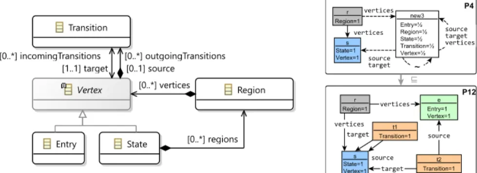
Fig. 1: Metamodel extract of Yakindu statecharts

Fig. 2: Partial models

and needs to be arranged into a strict containment hierarchy while graphs of the semantic web may be flat and nodes may have multiple types. Such restrictions will be introduced later as structural constraints. Mathematically, partial models show close resemblance with graph shapes [75, 76].

If a 3-valued partial modelP only contains 1 and 0 values, and there is no

∼relation between different objects (i.e. all equivalent nodes are merged), then P also represents aconcrete instance model M.

Example 1. Figure 1 shows a metamodel extracted from Yakindu statecharts whereRegionscontainVertexesandTransitions(leading from asourcever- tex to atargetvertex). An abstract stateVertexis further refined intoStates andEntrystates whereStatesare further refined intoRegions.

Figure 2 illustrates two partial models:P4, P12 (to be derived by the refine- ment approach in Section 4). The truth value of the type predicates are denoted by labels on the nodes, where 0 values are omitted. Reference predicate values 1 and¹/2 are visually represented by edges with solid and dashed lines, respec- tively, while missing edges between two objects represent 0 values for a predicate.

Finally, uncertain¹/2equivalences are marked by dashed lines with an∼symbol, while certain equivalence self-loops on objects are omitted.

Partial modelP4 contains one (concrete)Regionr, oneState s, and some other objects collectively represented by a single node new3. Object s is both of typeStateandVertex, whilenew3 represents objects with multiple possible types. Objectsis linked fromrvia averticesedge, and there are other possible references between randnew3. Partial modelP12, which is a refinement ofP4, has no uncertain elements, thus it is also a concrete instance modelM.

3.3 Graph patterns as well-formedness constraints

In many industrial modeling tools, complex structural WF constraints are cap- tured either by OCL constraints [70] or by graph patterns (GP) [11,49,67]. Here, we use a tool-independent first-order graph logic representation (which was in-

[[C(v)]]^P_Z:=IP(C)(Z(v)) [[R(v1, v2)]]^P_Z:=IP(R)(Z(v1), Z(v2))

[[v1∼v2]]^P_Z:=IP(∼)(Z(v1), Z(v2)) [[φ1∧φ2]]^P_Z:=min([[φ1]]^P_Z,[[φ2]]^P_Z) [[φ1∨φ2]]^P_Z:=max([[φ1]]^P_Z,[[φ2]]^P_Z)

[[¬φ]]^P_Z:=1−[[φ]]^P_Z

[[∃v:φ]]^P_Z:=max{[[φ]]^P_Z,v↦→x:x∈Obj_P} [[∀v:φ]]^P_Z:=min{[[φ]]^P_Z,v↦→x:x∈Obj_P}

Fig. 3: Semantics of graph patterns (predicates) Fig. 4: Malformed model

fluenced by [76, 98] and is similar to [85]) that covers the key features of several existing graph pattern languages and a first-order logic (FOL) fragment of OCL.

Syntax. A graph pattern (or formula) is a first order logic (FOL) formula φ(v1, . . . , vn) over (object) variables. A graph pattern φ can be inductively constructed (see Figure 3) by using atomic predicates of partial models: C(v), R(v₁, v₂),v₁∼v₂, standard FOL connectives ¬,∨, ∧, and quantifiers∃ and∀.

A simple graph pattern only contains (a conjunction of) atomic predicates.

Semantics. A graph patternφ(v1, . . . , vn) can be evaluated on partial modelP along a variable binding Z, which is a mapping Z :{v1, . . . , vn} →Obj_P from variables to objects in P. The truth value of φcan be evaluated over a partial model P and mappingZ (denoted by [[φ(v1, . . . , vn)]]^P_Z) in accordance with the semantic rules defined in Figure 3. Note that min and maxtakes the numeric minimum and maximum values of 0,¹/2 and 1 with 0≤¹/2≤1, and the rules follow 3-valued interpretation of standard FOL formulae as defined in [76, 85].

A variable bindingZ is called amatchif the patternφis evaluated to 1 over P, formally [[φ(v1, . . . , vn)]]^P_Z = 1. If there exists such a variable bindingZ, then we may shortly write [[φ]]^P = 1. Open formulae (with one or more unbound vari- ables) are treated by introducing an (implicit) existential quantifier over unbound variables to handle them similarly to graph formulae for regular instance models.

Thus, in the sequel, [[φ(v1, . . . , vn)]]^P_Z = 1 if [[∃v1, . . . ,∃vn:φ(v1, . . . , vn)]]^P = 1 where the latter is now a closed formula without unbound variables. Simi- larly, [[φ]]^P = ¹/2 means that there is a potential match where φ evaluates to ¹/2, i.e. [[∃v₁, . . . ,∃v_n:φ(v₁, . . . , v_n)]]^P = ¹/2, but there is no match with [[φ(v1, . . . , vn)]]^P_Z = 1. Finally, [[φ]]^P = 0 means that there is surely no match, i.e.

[[∃v1, . . . ,∃vn:φ(v1, . . . , vn)]]^P = 0 for all variable bindings. Here∃v1, . . . ,∃vn : φ(v₁, . . . , v_n) abbreviates∃v1: (. . . ,∃vn:φ(v₁, . . . , v_n)).

The formal semantics of graph patterns defined in Figure 3 can also be eval- uated on regular instance models with closed world assumption. Moreover, if a partial model is also a concrete instance model, the 3-valued and 2-valued truth evaluation of a graph pattern is unsurprisingly the same, as shown in [85].

Proposition 1. Let P be a partial model which is simultaneously an instance model, i.e.P =M. Then the 3-valued evaluation of anyφonP and its 2-valued evaluation onM is identical, i.e.[[φ]]^P_Z = [[φ]]^M_Z along any variable binding Z.

Graph patterns as WF constraints. Graph patterns are frequently used for defin- ing complex structural WF constraints and validation rules [96]. Those con- straints are derived from two sources: the metamodel (or type graph) defines core structural constraints, and additional constraints of a domain can be defined by using nested graph conditions [40], OCL [70] or graph pattern languages [96].

When specifying a WF constraint ϕ by a graph pattern φ, pattern φ cap- tures the malformed case by negatingϕ, i.e.φ=¬ϕ. Thusa graph pattern match detects a constraint violation. Given a set of graph patterns {φ1, . . . , φ_n} con- structed that way, a consistent instance model requires that no graph pattern φ_ihas a match inM. Thus any matchZ for any patternφ_i with [[φ_i]]^M_Z = 1 is a proof of inconsistency. In accordance with the consistency definitionM |=WF of Section 2,WF can defined by graph patterns asWF =¬φ₁∧. . .∧ ¬φ_n.

Note that consistency is defined above only for instance models, but not for partial models. The refinement calculus to be introduced in Section 4 ensures that, by evaluating those graph patterns over partial models, the model genera- tion will gradually converge towards a consistent instance model.

Example 2. The violating cases of two WF constraints checked by the Yakindu tool can be captured by graph patterns as follows:

– incomingToEntry(v) :Entry(v)∧ ∃t:target(t, v)

– noEntryInRegion(r) :Region(r)∧ ∀v:¬(vertices(r, v)∧Entry(v)) Both constraints are satisfied in instance model P12 as the corresponding graph patterns have no matches, thusP12 is a consistent result of model gener- ation. On the other hand, P₁₀ in Figure 4 is a malformed instance model that violates constraintincomingToEntry(v) along objecte:

[[incomingToEntry(v)]]^P_v↦→e¹⁰ = 1 and [[noEntryInRegion(r)]]^P10 = 0 While graph patterns can be easily evaluated on concrete instance models, checking them over a partial model is a challenging task, because one partial model may represent multiple concretizations. It is shown in [85] how a graph patternφcan be evaluated on a partial modelP with 3- valued logic and open- world semantics using a regular graph query engine by proposing a constraint rewriting technique. Alternatively, a SAT-solver based approach can be used as in [24, 31] or the general or initial satisfaction can be defined for positive nested graph constraints as in [41, 82].

4 Refinement and Concretization of Partial Models

Model generation is intended to be carried out by a sequence of refinement steps which starts from a generic initial partial model and gradually derives a

concrete instance model. Since our focus is to derive consistent models, we aim at continuously ensuring that each intermediate partial model can potentially be refined into a consistent model, thus a partial model should be immediately excluded if it cannot be extended to a well-formed instance model.

4.1 A refinement relation for partial model generation

In our model generation, the level of uncertainty is aimed to be reduced step by step along a refinement relation which results in partial models that represent a fewer number of concrete instance models than before. In a refinement step, predicates with¹/2values can be refined to either 0 or 1, but predicates already fixed to 1 or 0 cannot be changed any more. This imposes an information ordering relationX⊑Y where eitherX =¹/2andY takes a more specific 1 or 0, or values ofX andY remain equal:X ⊑Y := (X =¹/2)∨(X =Y).

Refinement from partial modelP to Q(denoted byP ⊑Q) is defined as a functionrefine :Obj_P →2^ObjQ which maps each object of a partial modelP to a non-empty set of objects in the refined partial model Q. Refinement respects the information ordering of type, reference and equivalence predicates for each p₁, p₂∈Obj_P and anyq₁, q₂∈Obj_Q withq₁∈refine(p₁),q₂∈refine(p₂):

– for each classCi: [[Ci(p1)]]^P ⊑[[Ci(q1)]]^Q;

– for each referenceRj: [[Rj(p1, p2)]]^P ⊑[[Rj(q1, q2)]]^Q; – [[p₁∼p₂]]^P ⊑[[q₁∼q₂]]^Q.

At any stage during refinement, a partial modelP can be concretized into an instance model M by rewriting all class type and reference predicates of value

1/2to either 1 or 0, and setting all equivalence predicates with¹/2to 0 between different objects, and to 1 on a single object. But any concrete instance model will still remain a partial model as well.

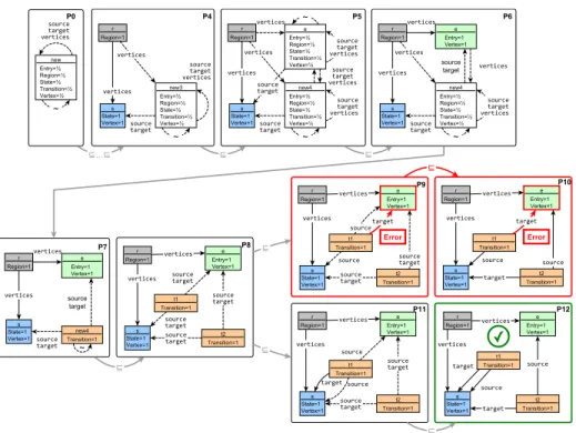
Example 3. Figure 5 depicts two sequences of partial model refinement steps deriving two instance models P₁₀ (identical to Figure 4) and P₁₂ (bottom of Figure 2):P₀⊑P₄⊑P₅⊑P₆⊑P₇⊑P₈⊑P₉⊑P₁₀andP₀⊑P₄⊑P₅⊑P₆⊑ P₇⊑P₈⊑P₁₁⊑P₁₂.

Taking refinement stepP₄ ⊑ P₅ as an illustration, object new3 (in P₄) is refined intoeandnew4 (inP5) where [[e∼new4]]^P5 = 0 to represent two different objects in the concrete instance models. Moreover, all incoming and outgoing edges of new3 are copied in e and new4. The final refinement step P11 ⊑ P12

concretizes uncertainsourceandtargetreferences into concrete references.

A model generation process can be initiated from an initial partial model provided by the user, or from the most generic partial model P₀ from which all possible instance models can be derived via refinement. Informally, thisP₀is more abstract than regular metamodels or type graphs as it only contains a single node as top-level class.P0contains one abstract object where all predicates are undefined, i.e.P0=⟨Obj_P0,IP₀⟩where Obj_P0 ={new}andIP₀ is defined as:

Fig. 5: Refinement of partial models

1. for all class predicates Ci: [[C_i(new)]]^P0 =¹/2;

2. for all reference predicatesRj: [[Rj(new,new)]]^P0 =¹/2.

3. [[new ∼new]]^P0 =¹/2to represent multiple objects of any instance model;

Our refinement relation ensures that if a predicate is evaluated to either 1 or 0 then its value will no longer change during further refinements as captured by the following approximation theorem.

Theorem 1. Let P, Qbe partial models with P ⊑Qandφbe a graph pattern.

– If [[φ]]^P = 1 then [[φ]]^Q = 1; if [[φ]]^P = 0 then [[φ]]^Q = 0 (called under- approximation).

– If [[φ]]^Q = 0 then [[φ]]^P ≤ ¹/2; if [[φ]]^Q = 1 then [[φ]]^P ≥ ¹/2 (called over- approximation).

If model generation is started from P₀ where all (atomic) graph patterns evaluate to ¹/2, this theorem ensures that if a WF constraintφis violated in a partial modelP then it can never be completed to a consistent instance model.

Thus the model generation can terminate along this path and a new refinement can be explored after backtracking. This theorem also ensures that if we evaluate a constraintφon a partial modelP and on its refinementQ, the latter will be more precise. In other terms, if [[φ]]^P = 1 (or 0) in a partial model P along

some sequence of refinement steps, then under-approximation ensures that its evaluation will never change again along that (forward) refinement sequence, i.e.

[[φ]]^Q = 1 (or 0). Similarly, when proceeding backwards in a refinement chain, over-approximation ensures monotonicity of the 3-valued constraint evaluation along the entire chain. Altogether, we gradually converge to the 2-valued truth evaluation of the constraint on an instance model where less and less constraints take the ¹/2value. However, a refinement step does not guarantee in itself that exploration is progressing towards a consistent model, i.e. there may be infinite chains of refinement steps which never derive a concrete instance model.

4.2 Refinement operations for partial models

We define refinement operations Op to refine partial models by simultaneously growing the size of the models while reducing uncertainty in a way that each finite and consistent instance model is guaranteed to be derived in finite steps.

– concretize(p, val): if the atomic predicatep(which is eitherCi(o),Rj(ok, ol) orok ∼ol) has a¹/2value in the pre-state partial modelP, then it can be refined in the post-stateQtovalwhich is either a 1 or 0 value. As an effect of the rule, the level of uncertainty will be reduced.

– splitAndConnect(o, mode): ifo is an object with [[o∼o]]^P =¹/2 in the pre- state, then a new objectnew is introduced in the post state by splitting o in accordance with the semantics defined by the following two modes:

• at-least-two: [[new∼new]]^Q=¹/2, [[o∼o]]^Q=¹/2, [[new∼o]]^Q= 0;

• at-most-two: [[new∼new]]^Q = 1, [[o∼o]]^Q= 1, [[new∼o]]^Q=¹/2; In each case,ObjQ=ObjP∪ {new}, and we copy all incoming and outgoing binary relations of o to new in Q by keeping their original values in P. Furthermore, all class predicates remain unaltered.

On the technical level, these refinement operations could be easily captured by means of algebraic graph transformation rules [28] over typed graphs. How- ever, for efficiency reasons, several elementary operations may need to be com- bined into compound rules. Thererfore, specifying refinement operations by graph transformation rules will be investigated in a future paper.

Example 4. RefinementP4⊑P5(in Figure 5) is a result of applying refinement operation splitAndConnect(o, mode) on object new3 and inat-least-two mode, splittingnew3 toeandnew4 copying all incoming and outgoing references. Next, in P₆, the type of object e is refined toEntry andVertex, the ¹/2equivalence is refined to 1, and references incompatible with Entry or Vertex are refined to 0. Note that in P₆ it is ensured that Regionrhas an Entry, thus satisfying WF constraint noEntryInRegion. In P₇ the type of object new4 is refined to Transition, the incompatible references are removed similarly, but the¹/2 self equivalence remain unchanged. Therefore, inP8 objectnew4 can split into two separate Transitions: t1 and t2 with the same source and target options. Re- finementP8⊑P9⊑P10denotes a possible refinement path, where thetargetof

t1 is directed to anEntry, thus violating WF constraintincomingToEntry. Note that this violation can be detected earlier in an unfinished partial modelP₉. Re- finementP₁₁⊑P₁₂ denotes the consecutive application of six concretize(p, val) operations on uncertain source and target edges leading out of t1 and t2 in P11, resulting in a valid model.

Note that these refinement operations may result in a partial model that is unsatisfiable. For instance, if all class predicates evaluate to 0 for an objectoof the partial model P, i.e. [[C(o)]]^P = 0, then no instance models will correspond to it as most metamodeling techniques require that each element has exactly or at least one type. Similarly, if we violate the reflexivity of ∼, i.e. [[o∼o]]^P = 0, then the partial model cannot be concretized into a valid instance model. But at least, one can show that these refinement operations ensure a refinement relation between the partial models of its pre-state and post-state.

Theorem 2 (Refinement operations ensure refinement).

Let P be a partial model and op be a refinement operation. If Q is the partial model obtained by executingopon P (formally,P −→^op Q) then P ⊑Q.

4.3 Consistency of model generation by refinement operations Next we formulate and prove the consistency of model generation when it is carried out by a sequence of refinement steps from the most generic partial model P0using the previous refinement operations. We aim to show soundness (i.e. if a model is derivable along an open derivation sequence then it is consistent), finite completeness (i.e. each finite consistent model can be derived along some open derivation sequence), and a concept of incrementality.

Many tableaux based theorem provers build on the concept of closed branches with a contradictory set of formulae. We adapt an analogous concept for closed derivation sequences over graph derivations in [28]. Informally, refinement is not worth being continued as a WF constraint is surely violated due to a match of a graph pattern in case of a closed derivation sequence. Consequently, all consistent instance models will be derived along open derivation sequences.

Definition 1 (Closed vs. open derivation sequence). A finite derivation sequence of refinement operations op1;. . .;opk leading from the most generic partial modelP0 to the partial modelPk (denoted asP0

op1;...;opk

−−−−−−→Pk) is closed wrt. a graph predicateφif φhas a match in Pk, formally, [[φ]]^Pk = 1.

A derivation sequence is open if it is not closed, i.e. Pk is a partial model derived by a finite derivation sequence P0

op₁;...;op_k

−−−−−−→Pk with[[φ]]^Pk ≤¹/2. Note that a single match of φ makes a derivation sequence to be closed, while an open derivation sequence requires that [[φ]]^Pk ≤¹/2which, by definition, disallows a match with [[φ]]^Pk≤1.

Example 5. Derivation sequence P0

−→... P9 depicted in Figure 5 is closed for φ=incomingToEntry(v) as the corresponding graph pattern has a match inP9,

i.e. [[incomingToEntry(v)]]^P_v↦→e⁹ = 1. Therefore,P₁₀ can be avoided as the same match would still exist. On the other hand, derivation sequence P₀ −→^... P₁₁ is open forφ=incomingToEntry(v) asincomingToEntry(v) is evaluated to¹/2in all partial modelsP0, . . . , P11.

As a consequence of Theorem 1, an open derivation sequence ensures that any prefix of the same derivation sequence is also open.

Corollary 1. LetP0

op1;...;opk

−−−−−−→Pk be an open derivation sequence of refinement operations wrt. φ. Then for each0≤i≤k,[[φ]]^Pi ≤¹/2.

The soundness of model generation informally states that if a concrete model M is derived along an open derivation sequence then M is consistent, i.e. no graph predicate of WF constraints has a match.

Corollary 2 (Soundness of model generation). Let P0

op₁;...;op_k

−−−−−−→Pk be a finite and open derivation sequence of refinement operations wrt. φ. If P_k is a concrete instance modelM (i.e.P_k =M) thenM is consistent (i.e.[[φ]]^M = 0).

Effectively, once a concrete instance modelM is reached during model gen- eration along an open derivation sequence, checking the WF constraints on M by using traditional (2-valued) graph pattern matching techniques ensures the soundness of model generation as 3-valued and 2-valued evaluation of the same graph pattern should coincide due to Proposition 1 and Theorem 1.

Next, we show that any finite instance model can be derived by a finite derivation sequence.

Theorem 3 (Finiteness of model generation).For any finite instance model M, there exists a finite derivation sequenceP0

op1;...;opk

−−−−−−→Pk of refinement oper- ations starting from the most generic partial modelP0 leading toPk=M.

Our completeness theorem states that any consistent instance model is deriv- able along open derivation sequences where no constraints are violated (under- approximation). Thus it allows to eliminate all derivation sequences where an graph predicateφ evaluates to 1 on any intermediate partial modelPi as such partial model cannot be further refined to a well-formed concrete instance model due to the properties of under-approximation. Moreover, a derivation sequence leading to a consistent model needs to be open wrt. all constraints, i.e. refinement can be terminated if any graph pattern has a match.

Theorem 4 (Completeness of model generation).For any finite and con- sistent instance model M with [[φ]]^M = 0, there exists a finite open derivation sequenceP0

op1;...;opk

−−−−−−→Pk of refinement operations wrt.φstarting from the most generic partial modelP0 and leading toPk=M.

Unsurprisingly, graph model generation still remains undecidable in general as there is no guarantee that a derivation sequence leading toPk where [[φ]]^Pk=

1/2 can be refined later to a consistent instance model M. However, the graph

model finding problem is decidable for a finite scope, which is an a priori upper bound on the size of the model. Informally, since the size of partial models is gradually growing during refinement, we can stop if the size of a partial model exceeds the target scope or if a constraint is already violated.

Theorem 5 (Decidability of model generation in finite scope). Given a graph predicate φ and a scope n ∈ N, it is decidable to check if a concrete instance modelM exists with|Obj_M| ≤nwhere[[φ]]^M = 0.

This finite decidability theorem is analogous with formal guarantees provided by the Alloy Analyzer [94] that is used by many mapping-based model generation approaches (see Section 6). Alloy aims to synthesize small counterexamples for a relational specification, while our refinement calculus provides the same for typed graphs without parallel edges for the given refinement operations.

However, our construction has extra benefits compared to Alloy (and other SAT-solver based techniques) when exceeding the target scope. First, all candi- date partial models (with constraints evaluated to ¹/2) derived up to a certain scope are reusable for finding consistent models of a larger scope, thus search can be incrementally continued. Moreover, if a constraint violation is found with a given scope, then no consistent models exist at all.

Corollary 3 (Incrementality of model generation).Let us assume that no consistent modelsMⁿ exist for scopen, but there exists a larger consistent model M^mof sizem(wherem > n) with[[φ]]^Mm = 0. ThenM^mis derivable by a finite derivation sequenceP_iⁿ −−−−−−−−→^{opi+1;...;opk} P_k^mwhereP_k^m=M^mstarting from a partial model P_iⁿ of size n.

Corollary 4 (Completeness of refutation). If all derivation sequences are closed for a given scope n, but no consistent model Mⁿ exists for scope n for which[[φ]]^Mn= 0, then no consistent models exist at all.

While these theorems aim to establish the theoretical foundations of a model generator framework, it provides no direct practical insight on the exploration itself, i.e. how to efficiently provide derivation sequences that likely lead to con- sistent models. Nevertheless, we have an initial prototype implementation of such a model generator which is also used as part of the experimental evaluation.

5 Evaluation

As existing model generators have been dominantly focusing on a single challenge of Section 2, we carried out an initial experimental evaluation to investigate how popular strategies excelling in one challenge perform with respect to another challenge. More specifically, we carried out this evaluation in the domain of Yakindu statecharts to address four research questions:

RQ1 Diverse vs. Realistic: How realistic are the models which are derived by random generators that promise diversity?

RQ2 Consistent vs. Realistic: How realistic are the models which are derived by logic solvers that guarantee consistency?

RQ3 Diverse vs. Consistent:How consistent are the models which are derived by random generators?

RQ4 Consistent vs. Scalable:How scalable is it to evaluate consistency constraints on partial models?

Addressing these questions may help advancing future model generators by identifying some strength and weaknesses of different strategies.

5.1 Setup of experiments

Target domain We conducted measurements in the context of Yakindu state- charts, see [2] for the complete measurement data. For that purpose, we ex- tracted the statechart metamodel of Figure 1 directly from the original Yakindu metamodel. Ten WF constraints were formalized as graph patterns based on the real validation rules of the Yakindu Statechart development environment.

Model generator approaches For addressingRQ1-3, we used two different model generation approaches: (1) the popular relational model finder Alloy Analyzer [94] which uses Sat4j [53] as a back-end SAT-solver, and (2) theViatraSolver, graph-based model generator which uses the refinement calculus presented in the paper. We selected Alloy Analyzer as the primary target platform as it has been widely used in mapping based generators of consistent models (see Section 6).

We operated these solvers in two modes: inconsistent mode (WF), all de- rived models need to satisfy all WF constraints of Yakindu statecharts, while in metamodel-only mode (MM), generated models need to be metamodel compli- ant, but then model elements are selected randomly. As such, we expect that this set of models is diverse, but the fulfillment of WF constraints is not guaranteed.

To enforce diversity, we explicitly check that derived models are non-isomorphic.

Since mapping based approaches typically compile WF constraints into logic formulae in order to evaluate them on partial models, we set up a simple mea- surement to addressRQ4 which did not involve model generation but only con- straint checking on existing instance models. This is a well-known setup for assessing scalability of graph query techniques used in a series of benchmark- ing papers [92, 98]. So in our case, we encoded instance models as fully defined Alloy specifications using the mapping of [86], and checked if the constraints are satisfied (without extending or modifying the statechart). As a baseline of comparison, we checked the runtime of evaluating the same WF constraints on the same models using an industrial graph query engine [97] which is known to scale well for validation problems [92, 98]. All measurements were executed on an average desktop computer⁶.

6 CPU: Intel Core-i5-m310M, MEM: 16GB, OS: Windows 10 Pro.

Real instance models To evaluate how realistic the synthetic model generators are in case ofRQ1-2, we took 1253 statecharts as real models created by un- dergraduate students for a homework assignment. While they had to solve the same modeling problem, the size of their models varied from 50 to 200 objects.

ForRQ4, we randomly selected 300 statecharts from the homework assignments, and evaluated the original validation constraints. Real models were filtered by removing inverse edges that introduce significant noise to the metrics [91].

Generated instance models To obtain comparable results, we generated four sets of statechart models with a timeout of 1 minute for each model but without any manual domain-specific fine-tuning of the different solvers. We also check that the generated models are non-isomorphic to assure sufficient diversity.

– Alloy (MM): 100 metamodel-compliant models with 50 objects using Alloy.

– Alloy (WF): 100 metamodel- and WF-compliant models with 50 objects using Alloy (which was unable to synthesize larger models within 1 minute).

– ViatraSolver (MM): 100 metamodel-compliant instance models with 100 objects usingViatraSolver.

– ViatraSolver (WF): 100 Metamodel- and WF-compliant instance models with 100 objects usingViatraSolver.

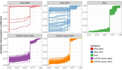
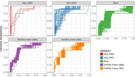
Two multi-dimensional graph metrics are used to evaluate how realistic a model generator is: (1) the multiplex participation coefficient (MPC) measures how the edges of nodes are distributed along the different edge types, while (2) pairwise multiplexity (Q)captures how often two different types of edges meet in an object. These metrics were recommended in [91] out of over 20 different graph metrics after a multi-domain experimental evaluation, for formal definitions of the metrics, see [91]. Moreover, we calculate the (3) number of WF constraints violated by a model as a numeric value to measure the degree of (in)consistency of a model (which value is zero in case of consistent models).

5.2 Evaluation of measurement results

We plot the distribution functions of themultiple participation coefficient metric in Figure 6, and the pairwise multiplexity metric in Figure 7. Each line depicts the characteristics of a single model and model sets (e.g. “Alloy (MM)”, “Viatra Solver (WF)”) are grouped together in one of the facets including the characteris- tics of the real model set. For instance, the former metric tells that approximately 65% of nodes in real statechart models (right facet in Figure 6) have only one or two types of incoming and outgoing edges while the remaining 35% of nodes have edges more evenly distributed among different types.

Comparison of distribution functions. We use visual data analytics techniques and the Kolmogorov-Smirnov statistic (KS) [55] as a distance measure of models (used in [91]) to judge how realistic an auto-generated model is by comparing the whole distributions of values (and not only their descriptive summary like

VIATRA Solver (MM) VIATRA Solver (WF)

Alloy (MM) Alloy (WF) Real

0.00 0.25 0.50 0.75 1.00 0.00 0.25 0.50 0.75 1.00

0.00 0.25 0.50 0.75 1.00 0.00

0.25 0.50 0.75 1.00

0.00 0.25 0.50 0.75 1.00

0.00 0.25 0.50 0.75 1.00 0.00

0.25 0.50 0.75 1.00

0.00 0.25 0.50 0.75 1.00

Multiplex Participation Coefficient

category Alloy (MM) Alloy (WF) Real

VIATRA Solver (MM) VIATRA Solver (WF)

Fig. 6: Measurement results: Multiplex participation coefficient (MPC)

mean or variance) in different cases to the characteristics of real models. The KS statistics quantifies the maximal difference between the distribution function lines at a given value. It is sensitive to both shape and location differences: it takes a 0 value only if the distributions are identical, while it is 1 if the values of models are in disjunct ranges (even if their shapes are identical). For comparing model generation techniques A and B we took the average value of the KS statistics between each (A, B) pair of models that were generated by technique A andB, respectively. The averageKS values are shown in Figure 9,⁷ where a lower value denotes a more realistic model set.

Diverse vs. Realistic: For the models that are only metamodel-compliant, the characteristics of the metrics for “ViatraSolver (MM)” are much closer to the

“Real” model set than those of the “Alloy (MM)” model set, for both graph metrics (KS value of 0.27 vs. 0.95 forMPC and 0.38 vs. 0.88 forQ), thus more realistic results were generated in the “Viatra Solver (MM)” case. However, these plots also highlight that the set of auto-generated metamodel-compliant models can be more easily distinguished from the set of real models as the plots of the latter show higher variability. Since the diversity of each model generation case is enforced (i.e. non-isomorphic models are dropped), we can draw as a conclusion thata diverse metamodel-compliant model generator does not provide any guarantees in itself on the realistic nature of the output model set. In fact, model generators that simultaneously ensure diversity and consistency always outperformed the random model generators for both solvers.

7 Due to the excessive amount of homework models, we took a uniform random sample of 100 models from that model set.

VIATRA Solver (MM) VIATRA Solver (WF)

Alloy (MM) Alloy (WF) Real

0.00 0.25 0.50 0.75 1.00 0.00 0.25 0.50 0.75 1.00

0.00 0.25 0.50 0.75 1.00 0.00

0.25 0.50 0.75 1.00

0.00 0.25 0.50 0.75 1.00

0.00 0.25 0.50 0.75 1.00 0.00

0.25 0.50 0.75 1.00

0.00 0.25 0.50 0.75 1.00

Pairwise Multiplexity

category Alloy (MM) Alloy (WF) Real

VIATRA Solver (MM) VIATRA Solver (WF)

Fig. 7: Measurement results: Pairwise multiplexity (Q)

0 50 100 150 200 250 300 350

0 50 100 150 200 250

Time (s)

Model Size (#Objects)

Validation by Alloy Validation by Graph Query Engine

Fig. 8: Measurement results: time of consistency checks: Alloy vs.ViatraSolver

model set MPC Q

Alloy (MM) 0.95 0.88

Alloy (WF) 0.74 0.60

ViatraSolver (MM) 0.27 0.37 ViatraSolver (WF) 0.24 0.30 Fig. 9: Average Kolmogorov-Smirnov statistics between therealand generated model sets.

Consistent vs. Realistic: In case of models satisfying WF constraints

“Viatra Solver (WF)” generated more realistic results than “Alloy (WF)” according to both metrics. The plots show mixed results for differen- tiating between generated and realis- tic models. On the positive side, the shape of the plot of auto-generated models is very close to that of real models in case of the MPC metric (Figure 6) – statistically, they have a

relatively low averageKSvalue of 0.24. However, for theQ metric (Figure 7), real

models are still substantially different from generated ones (average KS value of 0.3). Thus further research is needed to investigate how to make consistent models more realistic.

Diverse vs. Consistent: We also calculated the average number of WF constraint violations, which was 3.1 for the “Alloy (MM)” case and 9.75 for the “Viatra Solver (MM)” case, while only 0.07 for real models. We observe that a diverse set of randomly generated metamodel-compliant instance models do not yield consistent models as some constraints will always be violated – which is not the case for real statechart models. In other terms, the number of WF constraint violations is also an important characteristic of realistic models which is often overseen in practice. As a conclusion, amodel generator should ensure consistency prior to focusing on increasing diversity. Since humans dominantly come up with consistent models,ensuring consistency for realistic models is a key prerequisite.

Consistent vs. Scalable: The soundness of consistent model generation inherently requires the evaluation of the WF constraints at least once for a candidate solu- tion. Figure 8 depicts the validation time of randomly selected homework models using Alloy and the VIATRA graph query engine wrt. the size of the instance model (i.e. the number of the objects). For each model, the two validation tech- niques made the same judgment (as a test for their correctness). Surprisingly, the diagram shows that the Alloy Analyzer scales poorly for evaluating constraints on medium-size graphs, which makes it unsuitable for generating larger models.

The runtime of the graph query engine was negligible at this scale as we expected based on detailed previous benchmarks for regular graph pattern matching and initial experiments for matching constraints over partial models [85].

While many existing performance benchmarks claim that they generate re- alistic models, most of them ignore WF constraints of the domain. According to our measurements, it is a major drawback since real models dominantly satisfy WF constraints while randomly generated models always violate some constraint.

This way, those model generators can hardly be considered realistic.

Threats to validity We carried out experiments only in the domain of stat- echarts which limits the generalizability of our results. Since statecharts are a behavioral modeling language, the characteristics of models (and thus the graph metrics) would likely differ from e.g. static architectural DSLs. However, since many of our experimental results are negative, it is unlikely that the Alloy gen- erator would behave any better for other domains. It is a major finding that while Alloy has been used as a back-end for mapping-based model generator approaches, its use is not justified from a scalability perspective due to the lack of efficient evaluation for complex structural graph constraints. It is also unlikely that randomly generated metamodel-compliant models would be more realistic, or more consistent in any other domains.

Concerning our real models, we included all the statecharts created by stu- dents, which may be a bias since students who obtained better grades likely

Logic Random Network Performance Real Solvers Generators Graphs Benchmarks Dataset

CON Model + − − + +

Complete 0 − − − −

DIV Model − + − − −

Set − + − − −

SCA

In Size − + + + +

In Quantity − ? + + −

REA Model - - - - +

Set − − − 0 +

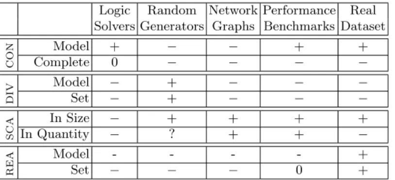
Table 1: Characteristics of model generation approaches; +: feature provided,−:

feature not provided, 0: feature provided in some tools / cases

produced better quality models. Thus, the variability of real statechart models created by engineers may actually be smaller. But this would actually increase the relative quality of models derived by ViatraSolver which currently differs from real models by providing a lower level of diversity (i.e. plots of pairwise multiplicity are thicker for real models).

6 Related work

We assess and compare how existing approaches address each challenge (Table 1).

Consistent model generators (CON): Consistent models can be synthesized as a side effect of a verification process when aiming to prove the consistency of a DSL specification. The metamodel and a set of WF constraints are captured in a high- level DSL and logic formulae are generated as input to back-end logic solvers.

Approaches differ in the language used for WF constraints, OCL [18–20, 23, 35, 50–52,73,87,100], graph constraints [84,86], Java predicates [14] or custom DSLs like Formula [46], Clafer [8] or Alloy [45]. They also differ inthe solver used in the background: graph transformation engines as in [100], SAT-solvers [53] are used in [51, 52], model finders like Kodkod [94] are target formalisms in [5, 23, 50, 87], first-order logic formulae are derived for SMT-solvers [65] in [73, 84] while CSP- solvers like [1] are targeted in [18, 19] or other techniques [59, 74].

Solver-based approaches excel in finding inconsistencies in specifications, while the generated model is a proof of consistency. While SAT solvers can handle specifications with millions of Boolean variables, all these mapping-based techniques still suffer from severe scalability issues as the generated graphs may contain less than 50-100 nodes. This is partly due to the fact that a Boolean variable needs to be introduced for eachpotential edge in the generated model, which blows up the complexity. Moreover, the output models are highly similar to each other and lack diversity, thus they cannot directly be applied for testing or benchmarking purposes.

Diverse model generators (DIV): Diverse models play a key role in testing model transformations and code generators. Mutation-based approaches [6, 25, 61] take existing models and make random changes on them by applying mutation rules.

A similar random model generator is used for experimentation purposes in [9].

Other automated techniques [15, 29] generate models that only conform to the metamodel. While these techniques scale well for larger models, there is no guar- antee whether the mutated models satisfy WF constraints.

There is a wide set of model generation techniques which provide certain promises for test effectiveness. White-box approaches [37, 38, 62, 83] rely on the implementation of the transformation and dominantly use back-end logic solvers, which lack scalability when deriving graph models. Black-box approaches [17, 34, 39, 56, 63] can only exploit the specification of the language or the trans- formation, so they frequently rely upon contracts or model fragments. As a com- mon theme, these techniques may generate a set of simple models, and while certain diversity can be achieved by using symmetry-breaking predicates, they fail to scale for larger model sizes. In fact, the effective diversity of models is also questionable since corresponding safety standards prescribe much stricter test coverage criteria for software certification and tool qualification than those currently offered by existing model transformation testing approaches.

Based on the logic-based Formula solver, the approach of [47] applies stochas- tic random sampling of output to achieve a diverse set of generated models by taking exactly one element from each equivalence class defined by graph isomor- phism, which can be too restrictive for coverage purposes. Stochastic simulation is proposed for graph transformation systems in [95], where rule application is stochastic (and not the properties of models), but fulfillment of WF constraints can only be assured by a carefully constructed rule set.

Realistic model generators (REA): The igraph library [22] contains a set of randomized graph generators that produce one-dimensional (untyped) graphs that follow a particular distribution (e.g. Erd˝os-R´enyi, Watts-Strogatz). The authors of [64] use Boltzmann samplers [27] to ensure efficient generation of uniform models. GSCALER [102] takes a graph as its input and generates a similar graph with a certain number of vertices and edges.

Scalable model generators (SCA): Several database benchmarks provide scalable graph generators with some degree of well-formedness or realism. The Berlin SPARQL Benchmark (BSBM)[13] uses a single dataset that scales in model size (10 million–150 billion tuples), but does not vary in structure. SP²Bench [80]

uses a data set, which is synthetically generated based on the real-world DBLP bibliography. This way, instance models of different sizes reflect the structure and complexity of the original real-world dataset.

The Linked Data Benchmark Council (LDBC) recently developed the So- cial Network Benchmark [30], which contains a social network generator mod- ule [88]. The generator is based on the S3G2 approach [72] that aims to generate non-uniform value distributions and structural correlations. gMark [7] generates