Cambodia: An autoregressive distributed lag approach
LEANGHAK HOK
PHD CANDIDATE
UNIVERSITY OF MISKOLC
PREK LEAP NATIONAL INSTITUTE OF AGRICULTURE
e-mail: leanghak.hok@gmail.com
SUMMARY
In the globalization age, global competitiveness is gaining attention from policymakers and scholars. This paper focuses on a measurement of trade competitiveness based upon the expansion of market size. Fiscal policy has become a subject of debate since the global crisis of 2008. This paper attempts to examine the influence of government spending (i.e., government investment and consumption) on trade competitiveness. The Autoregressive Distributed Lags (ARDL) approach is used to estimate the dynamic relationship. The result, based on Cambodia's annual data from 1970 to 2015, shows that Cambodia’s trade competitiveness increases when there is a rise in public investment, government purchases, or aggregate private spending. This study shapes an alternative perception of the effectiveness of fiscal policy as domestic expenditure in enhancing international macroeconomic activities.
Keywords: Competitiveness; public investment; government consumption; ARDL approach; Cambodia JEL classification: C50, C80, E62, F62, H50
DOI: http://dx.doi.org/10.18096/TMP.2020.02.03
I NTRODUCTION
Competitiveness can be identified as the set of institutions (e.g., private and public institutions), policies (e.g., fiscal and monetary policy), and other economic factors (e.g., export and infrastructure) influencing the productivity in a country (Cann, 2016).
A country’s competitiveness is a basis for enhancing the level of well-being. The competitiveness of the economy is credited with its productivity. The elevation of productivity level reflects economic growth, which boosts the income level and therefore the level of well- being. Traditionally, one aspect of competitiveness is considered to be domestic producers’ capacity relative to foreign producers in the term of substitution goods and services. The fluctuation in the nominal exchange rate of the home country and its trading partners leads to a change in trade competitiveness. The real exchange rate has been used as a measure for international competitiveness in a few studies (e.g., Makin and Ratnasiri (2015) and Nagayasu (2017)).
Many economic indicators affect the competitiveness of the economy. From a macroeconomic aspect, a wide range of factors (i.e.,
changes in the wage level, monetary and fiscal policy intervention made by the home country or by foreign countries) influences competitiveness. Fleming (1962) and Mundell (1963) analyze the efficiency of monetary and fiscal policy in an open economy to competitiveness. Under a flexible exchange rate system, an expansion of monetary policy improves not only competitiveness but also the trade balance. The stimulation of fiscal policy (government spending) financed by government borrowing appreciates the real exchange rate and negatively affects the trade balance due to an increase in interest rates, thereby hurting trade competitiveness. Mankiw (2012) discusses the notion of twin deficit. National savings decline just as government spending goes up, thus raising the real interest rates.
Higher real interest rates generate more capital in the domestic capital market and therefore cause a fall in the net capital outflow. The appreciation of the real exchange rate (loss of international competitiveness) occurs in response to a decline in net capital outflow, which also has a negative effect on the trade account balance.
Historical research mostly investigated the reaction of the real exchange rate to interest parity, interest rates, monetary policy, price level, and purchasing power
rather than to fiscal variables. Paradigmatic studies conducted by Dornbusch (1975) and Monacelli and Perotti (2010) concern the influence of fiscal policy on international trade in the field of international macroeconomics and also suggest the existence of a linkage between government spending and the real exchange rate. The empirical literature, meanwhile, refers to effective fiscal policy and only explores the connection between fiscal balance and current accounts (a survey in Abbas et al. 2011). Some of the empirical research spotlight government expenditure-real exchange rate linkage. The revaluation of the real exchange rate responds to a rise in government purchases (Chen & Liu, 2018; Chinn, 1999; De Gregorio et al., 1994). Some scholars show a different result. The expansion of government purchases improves productivity and employment and also devalues the real exchange rate of a country (Corestti el al., 2012; Dellas et al., 2005; Kollmann, 2010; Makin &
Ratnasiri, 2015; Ravn et al., 2007).
In the early 2010s, Cambodia’s real effective exchange rate index continuously dropped (as seen in Figure 1). At the same time, government fixed capital formation (public investment) as a share of GDP declined from 8.20 percent in 2010 to 5.30 percent in 2015. Government final consumption expenditure as a share of GDP decreased from 6.34 percent in 2010 to 5.39 percent in 2015. The reduction of government spending during this period may have led to less incentive for investment and thus reduced private consumption in Cambodia. Household final consumption expenditure as a share of GDP went down from 81.29 percent in 2010 to 76.80 percent in 2015.
This situation leads to lower relative money demand in Cambodia, thereby appreciating the real exchange rate or triggering a decline in the real effective exchange rate index. Thus, fiscal policy in Cambodia may contribute to the real effective exchange rate index. It is necessary to know how government spending influences the real exchange rate.
Nonetheless, this study deals only with one aspect of competitiveness derived from the expansion of the market size (i.e., a combination of the domestic and foreign markets) and focuses on the different types of government spending. For this kind of analysis, the best measurement for trade competitiveness is the real effective exchange rate (seen in the theoretical and empirical literature). This paper aims to investigate one aspect of competitiveness as trade competitiveness and the effect of government spending (i.e., public investment and government consumption) on trade competitiveness in Cambodia. The paper is structured as follows. Section 2 describes a measurement of trade competitiveness, the calculation of the real effective exchange rate index, and related research. Section 3 offers the competitiveness trend in the Cambodia context. Section 4 presents a hypothesis. The specific model, data collection, and method are presented in Section 5. Section 6 highlights results and discussion.
Section 7 contains conclusions and policy implications.
L ITERATURE REVIEW
A measurement of trade competitiveness
Most countries in the world are open economies.
Globalization (i.e., the interdependence between countries or the openness of the economy to the world market) leads to the integration of national economies through culture, information technology, investment, and international trade. In a globalized economy, the extension of market size through international trade can be a potential indicator of trade competitiveness. The expansion of the market for produced goods and services encourages the trade competitiveness of a country. That is, lower prices on those goods and services and a higher level of aggregate productivity react to a larger market size due to higher elasticity of demand in the market. Remarkably, the market size is a critical pillar for determining global competitiveness, according to the global competitiveness report 2017- 2018 (Schwab, 2017). With ceteris paribus, a change in foreign market size depends on a price level in foreign currency. If the foreign prices (prices in trading partners’ currency) of goods and services produced in the home country are low relative to trading partners, the foreign market for these goods and services increases.
The domestic price of products can represent the lowest cost of production at that place because producers can use economies of scale (i.e., a reduction in cost per unit as a response to an increase in the total output of production) to implement a low-price strategy in a competitive market (Samuelson, 1984). The domestic price measured in home currency can be expressed in a foreign currency with the help of the nominal exchange rate used to compute the real exchange rate in order to compare price levels between countries. An elastic real exchange rate creates elastic market size and thus trade competitiveness because a change in the real exchange rate can change the prices in foreign markets relative to those of the trading partners. The real exchange rate, therefore, can also be an alternative measurement of trade competitiveness. The clear connection between prices and cost competitiveness is measured with the help of the real exchange rate (Lipschitz & McDonald, 1992). An improvement in the cost competitiveness of international airlines is the result of the depreciation of the real exchange rate in the home country (Forsyth &
Dwyer 2010). Makin and Ratnasiri (2015) and Nagayasu (2017) use the real exchange rate to measure the trade competitiveness of a country. An appreciation of the real exchange rate weakens the trade competitiveness of the economy while the devaluation of the real exchange boosts it. For example, the global competitiveness of companies from the USA improved in response to the devaluation of the US dollar between 2002 and 2008, thereby opening up education (skill development), employment, and investment opportunities (Baily & Slaughter, 2008).
The real effective exchange rate refers to the weighted average of the home currency against a basket of primary trading partners’ foreign currencies. The Asian Development Bank (ADB) reports in own database that Cambodia regularly exports to ten trading partners (i.e., Belgium, Canada, Hong Kong, Germany, Japan, the People’s Republic of China, Spain, Thailand, the United Kingdom, and the United States of America (USA)). The export value of these ten trading partners in 2010 was approximately 78 percent of Cambodia's total export. The bilateral real exchange rate can be computed by the formula below (Catão, 2007):
it it*
it
t
E P
RER P
= × ,
(1) where t =1970, 1971,…, 2015;
i=1, 2,…,10 stands for trading partners;
RERit denotes the bilateral real exchange rate of the Riel (Cambodia’s currency) against a foreign currency i at the time t;
Eit represents the nominal exchange rate measured by the AMA exchange rate (Riel/foreign currency i) at the time t;
it*
P stands for the price level in a foreign country i at the time t;
Pt refers to the price level in Cambodia (home country) at the time t.
There are only data for the nominal exchange rate of the foreign currency of the country i against the US dollar; data of the nominal exchange rate of Cambodia currency against the foreign currency of the other countries is unavailable. The transformation can be made with this formula:
, USA t it
it
E E
= e
(2) where EUSA t, denotes the nominal exchange rate of the
Riel against the US dollar at the time t; eit stands for the nominal exchange rate of the foreign currency iagainst the US dollar at the time t.
The consumer price index (CPI) at 2010=100 is used as a proxy for the price level. In the case of states without available data of CPI (i.e., Cambodia, Hong Kong, and the People's Republic of China), a GDP deflator acts as a proxy for the price level.
To transform the real exchange rate into the index primarily relies on setting up the base year. Basing on the base year 2010, we get 100 as an index value of the bilateral real exchange rate in 2010. The bilateral real exchange rate index can be calculated as follows:
,2010 it 100
it
i
RER Index RER
RER
= ×
(3) where RERi,2010 is the real exchange rate of the Riel
against the foreign currency i in 2010.
These bilateral real exchange rate indices can be converted into a real effective (multilateral) exchange rate index as follows:
( )
10
1
wi
t it
i
R RER Index
=
=
∏
(
RER Indexit) (
w1 RER Indexit)
w2 ...(
RER Indexit)
w10= × × ×
(4) where Rt stands for the real effective exchange rate
index at the time t;
wi denotes the export-weighted index for the country i.
These weights based on bilateral exports as a share of total exports in 2010 are calculated to estimate Cambodia’s real effective exchange rate index. The export-weighted index can be computed as follows:
i i
w BE
= TE
(5) where BEi represents bilateral exports between
Cambodia and the country i in 2010;
TE denotes Cambodia’s total exports in 2010.
Cambodia’s exchange rate is written as a home currency against a foreign currency. A higher real effective exchange rate index can be interpreted as the depreciation of the real exchange rate, thereby improving trade competitiveness. The nominal exchange rate and GDP deflator at 2010=100 are taken from the National Accounts Main Aggregates Database, United Nations. CPI at 2010=100 and export data in 2010 are retrieved from the World Bank Indicators and the ADB database, respectively.
Related research
The Redux model (two-country model) developed by Obstfeld and Rogoff (1995) is based on macroeconomic dynamics of supply framework with some assumptions (e.g., monopolistic competition and price stickiness). Nominal producer prices in the short run are set in advance. Under rigid prices, output equals aggregate demand for the economy. Under monopolistic competition, producer prices are higher than the marginal cost, thus producing profits for producers.
With the preset price in the home currency of the producers, the producers’ output price in terms of the foreign currency fluctuates in response to a change in the exchange rate. The stimulation of home government
spending generates a decline in domestic consumption relative to foreign consumption since residents in the home country have to pay taxes used to finance government spending. The relative demand for money in the home country has higher fluctuation than the relative consumption, thus leading to the depreciation of the real exchange rate and thus improvement of trade competitiveness. Di Giorgio et al. (2018) also develop a two-country model with different assumptions from Obstfeld and Rogoff (1995). Their assumptions are non- Ricardian households and productive government purchases. Non-Ricardian households can be identified as households consuming based on current income and not taking out a loan to smooth their consumption (Céspedes et al., 2012; Coenen & Straub, 2005; Marto, 2014). In the case of productive government purchases, a rise in government spending causes a positive externality on the productivity of the private sector. The stimulation of government spending improves labor productivity in the private sector and influences marginal costs and inflation through demand-side and supply-side channels. In the demand-side channel, higher aggregate demand leads to inflationary pressure.
In the supply-side channel, domestic inflation and marginal costs decline in response to higher productivity in the private sector. The non-Ricardian structure of this model leads to expansionary public policy with an unbalanced budget in each period. Households, therefore, arrange their savings to buy a government bond, thereby not disturbing their future consumption.
With non-Ricardian households, the demand-side channel is relatively weak compared to the supply-side channel because the change in household consumption generates only a small change in aggregate demand.
The final result, therefore, is a fall in domestic inflation.
A decline in domestic inflation provokes a decrease in the local interest rates due to the monetary policy response, thereby depreciating the real exchange rate and enhancing trade competitiveness.
Makin and Ratnasiri (2015) studied the reaction of competitiveness to the extension of government spending in Australia. Two types of goods (tradable and non-tradable goods) are supposed in the Australian economy. The real exchange rate is the ratio of domestic currency price of non-traded to traded goods. Non- traded goods and services (e.g., electricity supply, water supply and so forth) refer to goods and services produced only for consumption in domestic economy and without making international trade (e.g., export and import) (Baxter et al., 1998; Sachs & Larrain, 1993;
Jenkins et al., 2011). Australia’s exchange rate is written as a foreign currency against the home currency,
thereby losing international competitiveness in response to a higher real exchange rate index. The expansionary government expenditure (i.e., public investment or consumption) on non-tradable goods leads to lower productivity growth in the tradable than the non-tradable goods sector. A decrease in opportunity cost of production resources (e.g., labor and capital) in non- tradable goods sector generates a reduction in the relative price of tradable goods. Therefore, the expansion of government spending on non-tradable goods sector appreciates the real exchange rate and thus weakens international competitiveness.
Based on a panel SVARs (structural vector autoregressive) approach and quarterly data from four developed countries (i.e., Australia, Canada, Sweden, and the United Kingdom), Bouakez and Eyquem (2015) indicated that the real exchange rate reacts to expansionary government spending by depreciating, thus intensifying international competitiveness. Kim (2015) used a panel VAR (vector autoregressive) approach with quarterly data from 18 developed countries and also found that the stimulus to government spending leads to the depreciation of the real exchange rate, thereby boosting international competitiveness.
On the other hand, Chen and Liu (2018) employed a small open economy model and a time-series SVARs approach and revealed that a rise in public investment or consumption appreciates the real exchange rate, thereby deteriorating the international competitiveness and trade balance and leading to the government’s twin deficit.
T RADE COMPETITIVENESS TREND IN THE CAMBODIAN CONTEXT
The data of the real effective exchange rate as a trade competitiveness measure are calculated to identify the trend. Figure 1 indicates the trend of the real effective exchange rate index over a period from 1970 to 2015.
The first national election organized by the United Nations Transitional Authority in Cambodia (UNTAC) in 1993 took place after Cambodia faced civil war during the period from 1970 to 1993. Subsequently, the Cambodian government had to increase its expenditure to rebuild the infrastructure and economy destroyed by this war. The real exchange rate grows sharply from 1988 to 1993. During 1988-1991, Vietnamese were detached from Cambodia, and there was a period of political unsettlement. The National Bank of Cambodia (NBC) therefore injected an enormous amount of money to settle the issue of the budget deficit.
Source: Author’s calculation
Figure 1. Cambodian real effective exchange rate index from 1970 to 2015
Cambodia adopted the managed floating exchange rate in 1993 (NBC, 2015). The real exchange rate also plays a principal role in Cambodia’s export
competitiveness (World Bank, 2015). Robust exports have also supported Cambodia’s strong economic growth during the last decade (ADB, 2018).
Source: National Accounts Main Aggregates Database, IMF Database, and author’s calculation
Note: Each dot depicts each year. Dashed line represents estimated line. Cambodian annual data are from 1970 to 2015.
Figure 2. Scatter (government spending, real effective exchange rate index) plot
As reported in panels (a) and (b) of Figure 2, two types of government expenditure (i.e., public investment
and government consumption) seem to contribute to the real effective exchange rate index in Cambodia.
0 5 10 15 20 25 30 35 40 45
Real effective exchange rate index
0 10 20 30 40 50 60
0 2 4 6 8 10
Real effective exchange rate index
Government fixed capital formation as a share of GDP (%)
Panel (a)
0 10 20 30 40 50 60
0 2 4 6 8 10 12 14 16 18 20
Real effective exchange rate index
Government final consumption expenditure as a share of GDP (%)
Panel (b)
H YPOTHESIS
According to the Redux model of Obstfeld and Rogoff (1995) and the two-country model developed by Di Giorgio et al. (2018), expansionary fiscal policy depreciates the real exchange rate and thus boosts trade competitiveness.This paper investigates the two types of government spending, such as government investment and consumption. The hypothesis of this paper suggests:
H: Government spending (i.e., public investment and consumption) positively affects trade competitiveness in Cambodia.
M ETHODOLOGY
Specific model
Household consumption and private investment play a crucial role in the fluctuation of the real exchange rate, as explained in the two-country models of Obstfeld and Rogoff (1995) and Di Giorgio et al. (2018). The recent research conducted by Makin and Ratnasiri (2015) also takes into account both the aggregate private spending and government spending in their model. Therefore, the international competitiveness function in this study can be written as follows:
(
,)
t t t
R = f E G
(6) where Rt stands for the real effective exchange rate
index at the time t,
Et refers to aggregate private spending (i.e., the sum of household consumption and private investment) at the time t,
Gt represents government spending at the time t.
Total government expenditure can be disaggregated into government consumption and public investment.
Notably, public investment significantly affects the supply side (production) for international competitiveness. The regression for this study, therefore, can be rewritten as follows:
0 1 2 3
t t t t t
R =
β
+β
E +β
GFCF +β
GFCE +ε
(7) where t= 1970, 1972… 2015,
Rt represents the real effective exchange rate index of Cambodia at the time t,
Et denotes aggregate private spending as a share of GDP of Cambodia at the time t,
GFCFt refers to government fixed capital formation as a share of GDP of Cambodia at the time t,
GFCEt stands for government final consumption expenditure as a share of GDP of Cambodia at the time t.
Data collection
Cambodia annual data obtained from1970 to 2015 create 46 observations. Variables used for this analysis are:
- Real effective exchange rate index: assessing cost competitiveness of the home country relative to the critical trading competitors;
- GDP at a constant price in 2011: the total value of goods and services produced per annum;
- Private investment at a constant price at 2011: the private sector’s investment spending in infrastructure services according to Investment and Capital Stock Dataset of IMF;
- Household final consumption expenditure as a share of GDP: the consumption of goods and services made by households and enterprises in the nation;
- Government fixed capital formation at a constant price 2011: acquisitions (i.e., purchase of new or second-hand assets) plus specific expenditure on services providing extra value to non-produced assets and then minus disposal of produced fixed assets;
- Government final consumption expenditure as a share of GDP: goods and services consumed by and collective consumption services offered by the general government.
The data for these variables are derived from two primary sources: the Investment and Capital Stock Dataset of the IMF and the National Accounts Main Aggregate Database of the United Nations. The link to obtain the data of GDP, government fixed capital formation, and private investment at a constant price at 2011 is:
https://www.imf.org/external/np/fad/publicinvestment/
For the rest of the variables mentioned above, data are accessed through the link below:
https://unstats.un.org/unsd/snaama/dnlList.asp
The conversions to receive explanatory variables for the regression are:
- Private investment and government fixed capital formation at a constant price 2011 divided by GDP at a constant price 2011 is equal to private investment as a share of GDP and government fixed capital formation as a share of GDP, respectively.
- Aggregate private spending as a share of GDP is the sum of household final consumption expenditure as a share of GDP and private investment as a share of GDP.
The data analysis is conducted in STATA 15.1 software.
Autoregressive Distributed Lags approach
The Engle–Granger approach (Engle & Granger, 1987) or Johansen's multivariate maximum likelihood approach for co-integration (Johansen, 1988; Johansen
& Juselius, 1990) requires all of the variables (i.e., dependent and independent variables) integrated to be order one I(1). The autoregressive distributed lags (ARDL) bound approach introduced by Pesaran and Shin (1998) and Pesaran et al. (2001) has several advantages over other traditional co-integration approaches. First, the ARDL model credibly deals with regressors with the existence of mutually integrated orders (zero I(0) and first I(1)) while the regressand is integrated of order one I(1) (Nkoro & Uko, 2016). Next, the ARDL model tests the existence of co-integration based on the standard F-test and estimates short-run and long-run relationships among explained and explanatory variables. Last, the ARDL approach also copes with the endogeneity problem by adding lags of explained and/or explanatory variables. Optimal lag lengths for ARDL bound test are selected under the minimum value of the Akaike Information Criterion (AIC) developed by Akaike (1977). The bound testing approach, based on the standard F-test with two sets of critical value (i.e., lower bound I(0) and upper bound I(1) ), justifies the existence of long-run co-integration. If the F-statistic estimated from the ARDL bound model is higher than the upper bound I(1), the null hypothesis, no co- integration, is rejected. In the case of an F-statistic between the lower and upper bound, no conclusion can be confirmed. An F-statistic lower than lower bound leads to the conclusion that long-run co-integration does not exist. If there is a long-run co-integration relationship among dependent and independent variables, a causal relationship exists, at least in one direction. We assumed unrestricted intercept and no trend in the equation of the ARDL bound test. The ARDL bound model of this study can be written as follows:
0 1 2 3 1
t t t t R t
R
β β
Eβ
GFCFβ
GFCEλ
ECT−∆ = + + + +
1 1 1
p k l
j t j j t j j t j
j j j
R E GFCF
θ − α − ϕ −
= = =
+
∑
∆ +∑
∆ +∑
∆1 k
j t j t
j
ρ
GFCE−ε
=
+
∑
∆ +(8) where ∆ represents the first difference,
λ
Rstands for the speed of adjustment, and ECTt-1 (error correction term) denotes disequilibrium. The coefficient of the error correction term indicates the speed to adjust disequilibrium due to short-run shocks to long-run equilibrium (Shahbaz et al. 2013). If this coefficient is statistically significant and negative, it depicts the existence of this adjustment. p,k
,l
, andm
refer to lags of ∆R, ∆E,∆ GFCF
, and∆ GFCE
, respectively. The selected value ofp,k
,l
, andm
is based on AIC.ε
t represents the error term. This study deals only with the long-run relationship between explained and explanatory variables and the effects ofEt, GFCFt, and GFCEt on Rt.
R ESULTS AND DISCUSSION Estimation
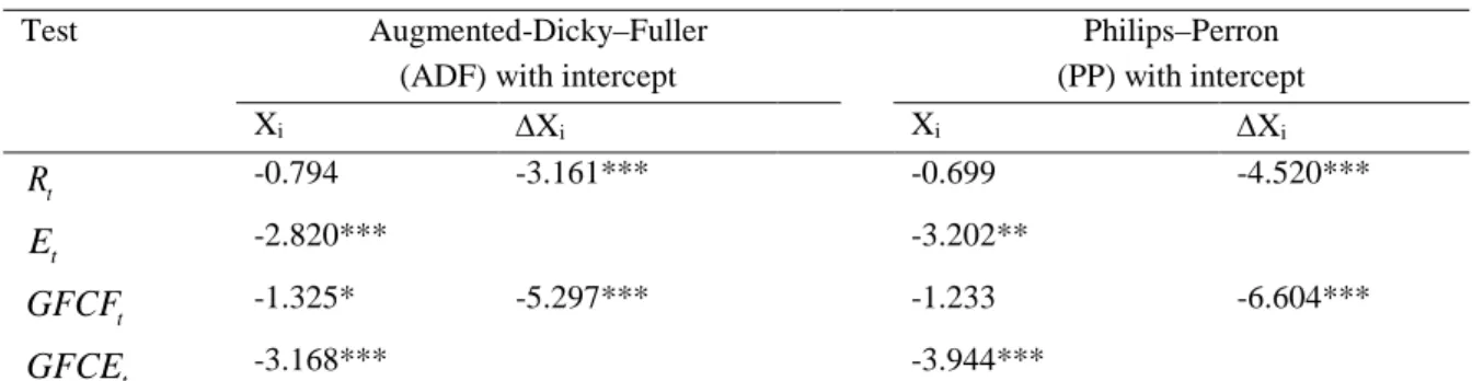
The analysis (e.g., OLS and ARDL approach) with the variables, non-stationarity after first differencing or without co-integration, generates a spurious result, thus demanding that a unit root test (stationary test) and co- integration test be conducted before running a regression (Granger & Newbold, 1973). The unit root test can be performed to reveal whether the time series has a deterministic trend (i.e., constant covariance, mean, and variance over time) or a stochastic trend (i.e., containing random walk) (Kirchgässner et al., 2013). If the unit-root exists, the variables have a stochastic trend.
This study employs two well-known unit root tests (i.e., Augmented-Dicky–Fuller suggested by Dickey and Fuller (1979) and Philips–Perron developed by Philips and Perron (1988)). The null hypothesis of both tests is unit-root (non-stationarity). The Augmented-Dicky–
Fuller (ADF) test relies heavily on the length of lags, therefore selecting the optimal lags based on the Bayesian Information Criterion (BIC) proposed by Schwarz (1978). The result of unit-root tests (ADF and Philips–Perron) seen in Table 1 reveals that the explained variable (Rt) is integrated of order one I(1).
The explanatory variable (GFCFt) has integration of order one I(1), but the other explanatory variables (Et
and GFCEt) are stationary at level I(0).
Test Augmented-Dicky–Fuller (ADF) with intercept
Philips–Perron (PP) with intercept
Xi ∆Xi Xi ∆Xi
Rt -0.794 -3.161*** -0.699 -4.520***
Et -2.820*** -3.202**
GFCFt -1.325* -5.297*** -1.233 -6.604***
GFCEt -3.168*** -3.944***
Note: ∆ donotes the first difference. * , **, and *** represent the significance level at 10, 5, and 1 percent, respectively. If both tests express stationarity, the variable is concluded as stationarity.
Dependent variable (
R
t)F Statistics 30.1126
Test critical value I(0) I(1)
1 percent level 4.29 5.61
5 percent level 3.23 4.35
10 percent level 2.72 3.77
Note: If F statistics is greater than the critical value of upper bound I(1), the null hypothesis is rejected.
Table 1 Unit root tests
The optimal lags chosen by AIC are 6 for the ARDL bound test. AIC also indicates 6, 5, 4, and 6 as the value of p, k, l, and m, respectively. The F-statistics shown in Table 2 are above the critical value of the upper bound
at a significance level of 1 percent. The null hypothesis of no co-integration, therefore, is rejected at these levels.
There is co-integration among these variables, so a causal relationship occurs in at least one direction.
Table 2
ARDL (6, 5, 4, 6) bound test for co-integration
The focus point of this study lies in the long-run relationship between government spending (i.e., public investment and consumption) and trade competitiveness. The long-run elasticity of the explained variable with respect to explanatory variables is reported in Table 3. Et, GFCFt and GFCEt are positive and statistically significant at these levels. The extension of aggregate private spending, public investment, or government consumption depreciates the real effective exchange rate, thereby gaining more trade competitiveness. The coefficient of error correction term (ECTt-1) is negative and significant at these levels.
The error-correction coefficient (λ = −R 0.334) indicates that the speed of adjustment– the period needed to return to the long-run equilibrium after disequilibrium in the short run – is approximately 33.4 percent.
The estimated result of the short-run implication is also presented in Table 3. Rt also reacts to its lags at a 1 percent significance level. A negative response of Rt to an increase of aggregate private spending, public investment, or government consumption is found in the short run, and these three variables are highly significant at these levels.
Rt
∆ ARDL (6, 5, 4, 6)
Coefficient Standard Error
Long-run
Et 7.546*** 0.450
GFCFt 17.208*** 0.682
GFCEt 17.483*** 0.860
Short-run
1
ECTt− -0.334*** 0.031
1
Rt−
∆ -0.726*** 0.128
2
Rt−
∆ -0.411*** 0.090
3
Rt−
∆ -0.182** 0.081
4
Rt−
∆ -0.286*** 0.065
5
Rt−
∆ -0.267** 0.095
Et
∆ -2.506*** 0.275
1
Et−
∆ -2.751*** 0.260
2
Et−
∆ -2.546*** 0.283
3
Et−
∆ -1.630*** 0.209
4
Et−
∆ -0.558*** 0.126
GFCFt
∆ -4.988*** 0.560
1
GFCFt−
∆ -3.729*** 0.436
2
GFCFt−
∆ -2.515*** 0.314
3
GFCFt−
∆ -0.876** 0.301
GFCEt
∆ -5.755*** 0.565
1
GFCEt−
∆ -5.738*** 0.540
2
GFCEt−
∆ -4.342*** 0.565
3
GFCEt−
∆ -1.741*** 0.367
4
GFCEt−
∆ 0.345 0.216
5
GFCEt−
∆ 0.540*** 0.138
Constant -285.156*** 30.615
Note:∆ denotes the first differences. *, ** and *** indicate the significance level at 10, 5, and 1 percent, respectively.
Table 3
Regression results from ARDL approach
Diagnostic tests
The key ARDL assumptions about the error term (residual) checked with diagnostic tests are no serial correlation, homoscedasticity, and normal distribution.
A residual has a serial correlation (i.e., the residual at time
t
correlates to the residual at the previous time), thus impacting the volume of t-statistics, standard error, and confident interval. Heteroscedasticity (i.e., the residual’s variance is not constant) implies that this built model does not explain the explained variable. If the residual is not a normal distribution, this model does notdescribe all trends of data. The Durbin–Watson test suggested by Durbin and Watson (1950) is carried out to check the residual. The null hypothesis is no serial correlation. The Breusch–Pagan test is used to confirm the residual with no heteroscedasticity as the test’s null hypothesis (Breusch & Pagan, 1979). The Jarque–Bera test introduced by Jarque and Bera (1987) joins between Skewness and Kurtosis. This test relies on asymptotic standard error without correlation for sample size. The normal distribution is proposed as the null hypothesis of the Jarque–Bera test. The three tests presented in Table 4 indicate that the null hypothesis of each test cannot be
ε
t Chi squaredDurbin–Watson test 0.446
Breusch–Pagan test 2.21
Jarque–Bera test 4.45
Note: *, **, and *** denotes the significance level at 10, 5, and 1 percent, respectively.
Cause
→
Effect Wald Statistics P-valueEt
→
Rt 5824.80*** 0.000
Rt
→
Et 163.58*** 0.000
GFCFt
→
Rt 2401*** 0.000
Rt
→
GFCFt 97.983*** 0.000
GFCEt
→
Rt 8502.6*** 0.000
R
→
GFCE 131.89*** 0.000Model ARDL (6, 5, 4, 6)
Test statistic 0.230
Critical value 1 percent 1.143
Critical value 5 percent 0.947
Critical value 10 percent 0.850
rejected at these levels. The residual of ARDL (6, 5, 4, 6) has no serial correlation, no heteroscedasticity, and normal distribution.
Table 4
Diagnostic tests of ARDL (6, 5, 4, 6)
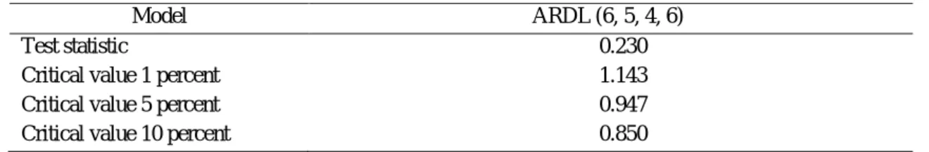
Stability test
The robustness of models can be checked with the cumulative sum test to confirm the parameter stability for the regression model. The cumulative sum test propounded in Brown et al. (1975) and based on recursive residuals is potentially designed to detect
instability of parameters (Ploberger & Krämer, 1992).
The null hypothesis of the cumulative sum test is no structural breaks (no change of regression coefficients over time). The result shown in Table 5 reveals the null hypothesis is not rejected at these levels of significance.
The estimated long-run parameters converge to the zero means, thereby leading to the existence of a stable and consistent model.
Table 5 Cumulative sum test
Causality test
The ARDL bound estimation does not disclose causality (i.e., cause and effect) among the considered variables. The Modified Wald test (MWALD) proposed by Toda and Yamamoto (1995) is carried out in this study to understand the directional causality relationship between government spending (i.e., public investment and consumption) and trade competitiveness. The MWALD, the so-called Toda–Yamamoto causality test, can manage problems (i.e., any possible non-stationarity or co-integration among variables) which the original Granger causality ignores (Wolde-Rufael, 2005). For
the Toda and Yamamoto (1995) approach, a standard vector autoregressive (VAR) model is applied to the level of variables rather than the first differences in the traditional Granger causality test, thus lessening the risks of wrongly identifying the integrated order of series (Mavrotas & Kelly, 2001). The null hypothesis of the Toda–Yamamoto causality test is no effect of a variable on another variable. The kaleidoscopic result of Toda–Yamamoto causality test is presented in Table 6.
The bi-directional causality relationship between three explanatory variables (i.e., aggregate private spending, public investment, and government consumption) and trade competitiveness is observed in this analysis.
Table 6
Toda–Yamamoto causality test result
Discussion
The result of public investment and government consumption in this study coincides precisely with the explanations of Obstfeld and Rogoff (1995) and Di Giorgio et al. (2018) based on the two-country model, that is to say, an increase in government spending improves trade competitiveness through depreciation of the real exchange rate as a measurement of trade competitiveness. This finding also agrees with the result of Bouakez and Eyquem (2015), who indicated that the response to the extension of public spending is the depreciation of the real exchange rate, which intensified international competitiveness in four developed countries. The result of this study is consonant with the result of Kim (2015), who suggested that the extension of government consumption in 18 industrialized countries enhances trade competitiveness owing to the improvement of the market size in response to the depreciation of the real exchange rate. Thus, the extension of the market size in the ear of globalization can be an effective channel for the improvement of trade competitiveness for developed and developing countries (e.g., Cambodia). The extension of government spending can encourage a level of productivity that generates low production cost and high relative money demand in the home country, so it is a benefit for expanding the market size and therefore increasing trade competitiveness.
The result of this study is inconsistent with the outcome of Makin and Ratnasiri (2015) due to the different baseline to reflect the real exchange rate as the measurement of trade competitiveness. The real exchange rate is the proportion of the domestic currency price of non-traded to traded goods. The improvement of the real exchange rate index appreciates Australia's currency and thus reduces the international competitiveness owing to Australia’s exchange rate written as a foreign currency against the home currency.
In the case of expansionary public policy (i.e., public investment and government purchase) on non-traded goods, real exchange rate appreciation responds to the growth in the relative price of non-traded goods (i.e., an increase in opportunity cost of tapping production resources in tradable goods sector) due to faster productivity growth in non-traded than traded goods sector. As a result, the extension of government expenditure on non-tradable goods sector decreases Australian international competitiveness. The finding of this study also is not in line with Chen and Liu (2018), who pointed that the enhancement of public investment or government consumption worsens the trade competitiveness due to the existence of the government’s twin deficit. While there are an increase in government expenditure and a decrease in national savings decrease, the real interest rates grow. More capital in the domestic capital market reacts to higher
real interest rates, thus reducing the net capital outflow.
A decline in net capital outflow decreases trade competitiveness via the appreciation of the real exchange rate and disrupts the trade account balance as well.
CONCLUSIONS AND POLICY IMPLICATIONS
Conclusions
Some scholars focus on the influence of public policy on trade competitiveness. This paper rigorously examines the reaction of trade competitiveness to the expansion of government spending (i.e., public investment and government consumption). The ARDL approach is employed to estimate dynamic relationships based on annual data from 1970 to 2015 from Cambodia. The result of this paper suggests that the extension of public investment or government purchases promotes trade competitiveness due to the devaluation of the real exchange rate. The result of aggregate private spending is the same as the result of public investment or government purchases. This study makes two contributes to international macroeconomic literature.
Firstly, in the term of the extension of market size, it indicates how a change in domestic spending impacts opened economy’s competitiveness through the real exchange rate. Lastly, international competitiveness based on the principle mentioned above is applied to Cambodian experience, thus revealing that a drop in Cambodia’s trade competitiveness over the period from 2011 to 2015 responded to a reduction in government spending.
Limitation
This study faces the problem of limited data.
Cambodia's historical data on public investment (GFCF) and government consumption (GFCE) from 1971 to 1986 seem to be unchanged. Cambodia was involved in a civil war at that period, so some of the data are the results of estimations by the United Nations and the IMF. This study only deals with one aspect of Cambodia’s trade competitiveness and is not a complex aspect of competitiveness. Monetary policy also contributes to price level, the nominal exchange rate and thus the real exchange rate. However, our model does not take into account it because the data of Cambodia’s money supply are limited.
Making use of quarterly (Makin & Ratnasiri, 2015) and semi-annual data can eliminate the effect of limited data. Alternatively, the panel data approach over ten countries in ASEAN is a solution for limited data.
Policy implications
The Cambodian government is making an effort to improve international competitiveness through the extension of market size, and thus Cambodia joined the World Trade Organization (WTO) in 2004. This outcome of this study depicts the efficacy of fiscal policy for Cambodia’s international macroeconomic activities via the real effective exchange rate. The expansion of government spending creates more incentive to invest in Cambodia and also enhances productivity via the improvement of labor productivity in the private sector. It can bring down the marginal cost of production and encourage private consumption in Cambodia. As a result, there is a high relative demand for money in Cambodia, thus leading to a depreciation of the real exchange rate and improving trade competitiveness. According to the result of this study, the Cambodia government can improve trade competitiveness through an expansionary fiscal policy (i.e., public investment and government purchases).
However, the efficacy of government spending may decrease if there are inefficient management of public investment and high corruption in the public sector.
Dabla-Norris et al. (2012) find that Cambodia’s PIMI
(Public investment management index) is 1.57. PIMI can be defined as the multi-dimension index of the efficiency and quality of public investment management process. The value of PIMI ranges between zero and four, and public investment is fully efficient when PIMI equals to 4. The Cambodia value (1.57) of this index means that a US dollar of public investment translates approximately 0.4 US dollars of capital in Cambodia.
The Cambodia corruption perception index is about 21 in the last six years (Quality of Government Institute, 2019) on a scale from 0 to 100 where 0 indicates the highest corruption and 100 means the perception is that there is no corruption in the public sector. Therefore, the government should take the initiative to improve the PIMI and the corruption perception indexes, thereby not offsetting the efficient and positive impact of government spending on trade competitiveness. The possibility for designing expansionary fiscal policy can be seen if there are high value of consolidated fiscal balance and low national debt. Cambodia’s consolidated fiscal balance as a share of GDP based on the CEIC database declined from -7.65 percent in 2011 to -2.66 percent in 2015. As reported by IMF’s database, Cambodia’s national debt as a share of GDP in the same period slightly increased from 30.30 percent to 32.54 percent.
Acknowledgments
The author would like to thank Dr. Zoltán Bartha for his valuable advice to improve this paper and the Hungarian government for financial support (through the Stipendium Hungaricum Scholarship) for doctoral studies. The author
also thanks anonymous referees for invaluable comments and suggestions to improve this paper.
REFERENCES
ABBAS, S. M. A. L. I., BOUHCA-HAGBE, J., FATÁS, A., MAURO, P., & VELLOSO, R. C. (2011). Fiscal Policy and the Current Account. IMF Economic Review, 59(4), 603–629.
ADB. (2018). ADB forecasts robust growth for Cambodia, sees risks to competitiveness. Retrieved April 10, 2019, from ADB website: https://www.adb.org/news/adb-forecasts-robust-growth-cambodia-sees-risks-competitiveness
AKAIKE, H. (1977). On entropy maximization principle. In P. R. Krishnaiah (Ed.), Application of Statistics (pp. 27–41).
Amsterdam: North-Holland Publishing company.
BAILY, M. N., & SLAUGHTER, M. J. (2008). Strengthening U. S. competitiveness in the global economy. Washington, D.C.: Private Equity Council. Retrieved from
http://mba.tuck.dartmouth.edu/pages/faculty/matthew.slaughter/pdf/PECouncil_rpt_1208.pdf
BAXTER, M., JERMANN, U. J., & KING, R. G. (1998). Nontraded goods, nontraded factors, and international non- diversification. Journal of International Economics, 44(2), 211–229.
https://doi.org/10.1016/S0022-1996(97)00018-4
BOUAKEZ, H., & EYQUEM, A. (2015). Government spending, monetary policy, and the real exchange rate. Journal of International Money and Finance, 56, 178–201. https://doi.org/10.1016/j.jimonfin.2014.09.010
BREUSCH, T. S., & PAGAN, A. R. (1979). A simple test for heteroscedasticity and random coefficient variation.
Econometrica, 47(5), 1287–1294. https://doi.org/10.2307/1911963
BROWN, R. L., DURBIN, J., & EVANS, J. M. (1975). Techniques for testing the constancy of regression relationships over time. Journal of the Royal Statistical Society: Series B (Methodological), 37(2), 149–192.
CANN, O. (2016). What is competitiveness? (27 Sep 2016) World Economic Forum website. Retrieved April 19, 2018, from: https://www.weforum.org/agenda/2016/09/what-is-competitiveness/
CATÃO, L. A. V. (2007, September). Why real exchange rates? Finance and Development, 44(3), 46–47. Retrieved from https://www.imf.org/external/pubs/ft/fandd/2007/09/pdf/basics.pdf
CÉSPEDES, L. F., FORNERO, J., & GALÍ, J. (2012). Non-Ricardian aspects of fiscal policy in Chile Working Papers Central Bank of Chile 663, Central Bank of Chile. Retrieved from https://core.ac.uk/download/pdf/6654271.pdf CHEN, Y., & LIU, D. (2018). Government spending shocks and the real exchange rate in China: Evidence from a sign-
restricted VAR model. Economic Modelling, 68, 543–554. https://doi.org/10.1016/j.econmod.2017.03.027
CHINN, M. D. (1999). Productivity, Government Spending and the Real Exchange Rate Evidence for OECD Countries.
In R. MacDonald & J. L. Stein (Eds.), Equilibrium Exchange Rates (Vol. 69, pp. 163–190).
/https://doi.org/10.1007/978-94-011-4411-7_6
COENEN, G., & STRAUB, R. (2005). Non-Ricardian households and fiscal policy in an estimated DSGE model of the Euro area. Computing in Economics and Finance 2005 (No. 102), Society for Computational Economics.
CORESTTI, G., MEIER, A., & MÜLLER, G. J. (2012). Fiscal stimulus with spending reversals. The Review of Economics and Statistics, 94(4), 878–895.
DABLA-NORRIS, E., BRUMBY, J., KYOBE, A., MILLS, Z., & PAPAGEORGIOU, C. (2012). Investing in public investment : An index of public investment efficiency. Journal of Economic Growth, 17(3), 235–266.
DE GREGORIO, J., GIOVANNI, A., & WOLF, H. C. (1994). International evidence on tradables inflation and nontradables. European Economic Review, 38, 1225–1244. https://doi.org/10.1016/0014-2921(94)90070-1
DELLAS, H., NEUSSER, K., & MANUEL, W. (2005). Fiscal Policy in Open Economies. Working Paper, Department of Economics (Switzerland: University of Bern).
DI GIORGIO, G., NISTICÒ, S., & TRAFICANTE, G. (2018). Government spending and the exchange rate. International Review of Economics and Finance, 54, 55–73. https://doi.org/10.1016/j.iref.2017.07.030
DICKEY, D. A., & FULLER, W. A. (1979). Distribution of the estimators for autoregressive time series with a unit root.
Journal of the American Statistical Association, 74(366), 427–431. https://doi.org/10.2307/2286348
DORNBUSCH, R. (1975). Exchange Rates and Fiscal Policy in a Popular Model of International Trade. The American Economic Review, 65(5), 859–871.
DURBIN, B. Y. J., & WATSON, G. S. (1950). Testing for serial correlation in Least Squares Regression : I. Biometrika, 37(3), 409–428.
ENGLE, R. F., & GRANGER, C. W. J. (1987). Co-integration and error correction: Representation, estimation, and testing. Econometrica, 55(2), 251–276. https://doi.org/10.2307/1913236
FLEMING, J. M. (1962). Domestic financial policies under fixed and under floating exchange rates. Palgrave Macmillan Journals on Behalf of the International Monetary Fund, 9(3), 369–380.
FORSYTH, P., & DWYER, L. (2010). Exchange rate changes and the cost competitiveness of international airlines: The Aviation Trade Weighted Index. Research in Transportation Economics, 26(1), 12–17.
https://doi.org/10.1016/j.retrec.2009.10.003
GRANGER, C. W. ., & NEWBOLD, P. (1973). Spurious regressions in eocnometrics. Journal of Econometrics, 2, 111–
120. https://doi.org/10.1002/9780470996249.ch27
JARQUE, C. M., & BERA, A. K. (1987). A test for normality of observations and regression residuals. International Statistical Review, 55(2), 163–172. https://doi.org/10.2307/1403192
JENKINS, G. P., KUO, C.-Y., & HARBERGER, A. C. (2011). Cost-benefit analysis for investment decisions: Chapter 11 (Economic prices for non-tradable goods and services). In JDI Executive Programs (No. 2011–11). Retrieved from https://cri-world.com/publications/qed_dp_204.pdf
JOHANSEN, S. (1988). Statistical analysis of cointegration vectors. Journal of Economic Dynamics and Control, 12(2–
3), 231–254. https://doi.org/10.1016/0165-1889(88)90041-3
JOHANSEN, S., & JUSELIUS, K. (1990). Maximum likelihood estimation and inference on cointegration—with applications to the demand for money. Oxford Bulletin of Economics and Statistics, 52(2), 169–210.
https://doi.org/10.1111/j.1468-0084.1990.mp52002003.x
KIM, S. (2015). Country characteristics and the effects of government consumption shocks on the current account and real exchange rate. Journal of International Economics, 97(2), 436–447. https://doi.org/10.1016/j.jinteco.2015.07.007 KIRCHGÄSSNER, G., WOLTERS, J., & HASSLER, U. (2013). Introduction to Modern Time Series Analysis (2nd ed.).
Berlin, Heidelberg: Springer-Verlag.
KOLLMANN, R. (2010). Government purchases and the real exchange rate. Open Economies Review, 21(1), 49–64.
https://doi.org/10.1007/s11079-009-9148-2
LIPSCHITZ, L., & MCDONALD, D. (1992). Real exchange rates and competitiveness. Journal of European Economics, 19(1), 37–69. https://doi.org/https://doi.org/10.1007/BF00924805
MAKIN, A. J., & RATNASIRI, S. (2015). Competitiveness and government expenditure: The Australian example.
Economic Modelling, 49, 154–161. https://doi.org/10.1016/j.econmod.2015.04.003
MANKIW, N. G. (2012). Principle of Macroeconomics (6th ed.). Mason: South-Western Cengage Learning.
MARTO, R. (2014). Assessing the impacts of non-Ricardian households in an estimated New Keynesian DSGE model.
Swiss Society of Economics and Statistics, 150(4), 353–398.
MAVROTAS, G., & KELLY, R. (2001). Old Wine in New Bottles: Testing causality between savings and growth. The Manchester School, 69(s1), 97–105. https://doi.org/10.1111/1467-9957.69.s1.6
MONACELLI, T., & PEROTTI, R. (2010). Fiscal Policy, the real exchange rate and traded goods. The Economic Journal, 120(544), 437–461. https://doi.org/10.1111/j.1468-0297.2010.02362.x
MUNDELL, R. A. (1963). Capital mobility and stabilization policy under fixed and flexible exchange rates. The Canadian Journal of Economics and Political Science, 29(4), 475–485. https://doi.org/10.2307/139336
NAGAYASU, J. (2017). Global and country-specific movements in real effective exchange rates: Implications for external competitiveness. Journal of International Money and Finance, 76, 88–105.
https://doi.org/10.1016/j.jimonfin.2017.05.005
NBC. (2015). Exchange rate policy. Retrieved April 8, 2018, from National Bank of Cambodia website:
https://www.nbc.org.kh/english/monetary_policy/exchange_rate_policy.php
NKORO, E., & UKO, A. K. (2016). Autoregressive Distributed Lag (ARDL) cointegration technique: application and interpretation. Journal of Statistical and Econometric Methods, 5(4), 63–91.
OBSTFELD, M., & ROGOFF, K. (1995). Exchange rate dynamics Redux. Journal of Political Economy, 103(3), 624–
660.
PESARAN, M. H., & SHIN, Y. (1998). An Autoregressive Distributed-Lag Modelling Approach to Cointegration Analysis. In S. Strøm (Ed.), Econometrics and Economic Theory in the 20th Century: The Ragnar Frisch Centennial Symposium (pp. 371–413). Cambridge: Cambridge University Press.
PESARAN, M. H., SHIN, Y., & SMITH, R. J. (2001). Bounds testing approaches to the analysis of level relationships.
Journal of Applied Econometrics, 16(3), 289–326. https://doi.org/10.1002/jae.616
PHILIPS, P., & PERRON, P. (1988). Biometrika trust testing for a unit root in time series regression. Biometrika, 75(2), 335–346. https://doi.org/10.1093/poq/nf1045
PLOBERGER, W., & KRÄMER, W. (1992). The CUSUM test with OLS residuals. Econometrica, 60(2), 271–285.
QUALITY OF GOVERNMENT INSTITUTE. (2019). QoG Standard Data. Quality of Government Institute, University of Gothenburg, Sweden. Retrieved June 12, 2019, from https://qog.pol.gu.se/data/datadownloads/qogstandarddata RAVN, M. O., SCHMITT-GROHÉ, S., & URIBE, M. (2007). Explaining the effects of government spending shocks on
consumption and the real exchange rate (No. 13328), NBER Working Papers. National Bureau of Economic Research. Retrieved from http://www.nber.org/papers/w13328
SACHS, J. D., & LARRAIN, F. B. (1993). Macroeconomics in the Global Economy (1st ed.). New Jersey: Prentice Hall.
(pp. 657-671)
SAMUELSON, P. A. (1984). Theoretical notes on trade problems. The Review of Economics and Statistics, 46(2), 145–
154.
SCHWAB, K. (2017). The Global Competitiveness Report 2017-2018. Geneva, Swizerland: World Economic Forum.
SCHWARZ, G. (1978). Estimating the dimension of a model. The Annals of Statistics, 6(2), 461–464.
https://doi.org/10.1214/aos/1176344136
SHAHbAZ, M., HYE, Q. M. A., TIWARI, A. K., & LEITÃO, N. C. (2013). Economic growth, energy consumption, financial development, international trade and CO 2 emissions in Indonesia. Renewable and Sustainable Energy Reviews, 25, 109–121. https://doi.org/10.1016/j.rser.2013.04.009
TODA, H., & YAMAMOTO, T. (1995). Statistical Inference in Vector Autoregressions with Possibly Integrated Processes. Journal of Econometrics, 66(1–2), 225–250.
WOLDE-RUFAEL, Y. (2005). Energy demand and economic growth: The African experience. Journal of Policy Modeling, 27(8), 891–903. https://doi.org/10.1016/j.jpolmod.2005.06.003
WORLD BANK. (2015). Maintaining high growth: Cambodia economic update (No. 95982). Retrieved from http://documents.worldbank.org/curated/en/881041467999363660/pdf/95982-REVISED-WP-PUBLIC-
Box391435B-Cambodia-Economic-Update-April-7-2015-Final.pdf