Neural networks would ‘vote’
according to Borda’s Rule
by Dávid Burka, Clemens Puppe, László Szepesváry and
Attila Tasnádi
C O R VI N U S E C O N O M IC S W O R K IN G P A PE R S
http://unipub.lib.uni-corvinus.hu/2498
CEWP 13 /201 6
Neural networks would ‘vote’
according to Borda’s Rule
D´avid Burka,(1) Clemens Puppe,(2) L´aszl´o Szepesv´ary(3) andAttila Tasn´adi(4) *
(1) Department of Mathematics, Corvinus University of Budapest, F˝ov´am t´er 8, H – 1093 Budapest, Hungary,dburka001@gmail.com
(2) Department of Economics and Management, Karlsruhe Institute of Technology, D – 76131 Karlsruhe, Germany,clemens.puppe@kit.edu
(3) Department of Operations Research and Actuarial Sciences, Corvinus University of Budapest, F˝ov´am t´er 8, H – 1093 Budapest, Hungary,szepesvaryl@gmail.com (4) MTA-BCE “Lend¨ulet” Strategic Interactions Research Group, Department of Mathematics, Corvinus University of Budapest, H – 1093 Budapest, F˝ov´am t´er 8,
Hungary,attila.tasnadi@uni-corvinus.hu
November 2016
Abstract Can neural networks learn to select an alternative based on a systematic aggregation of conflicting individual preferences (i.e. a ‘voting rule’)? And if so, which voting rule best describes their behavior? We show that a prominent neural network can be trained to respect two fundamental principles of voting theory, the unanimity principle and the Pareto property. Building on this positive result, we train the neural network on profiles of ballots possessing a Condorcet winner, a unique Borda winner, and a unique plurality winner, respectively. We investigate which social outcome the trained neural network chooses, and find that among a number of popular voting rules its behavior mimics most closely the Borda rule. Indeed, the neural network chooses the Borda winner most often, no matter on which voting rule it was trained. Neural networks thus seem to give a surprisingly clear-cut answer to one of the most fun- damental and controversial problems in voting theory: the determination of the most salient election method.
Keywords: voting, social choice, neural networks, machine learning, Borda count.
*This work has been presented at the Workshop on Game Theory and Social Choice (Budapest, December 2015), at the Workshop on Voting Theory and Social Choice (Berlin, June 2016), at the COMSOC Conference (Toulouse, June 2016), and at the 13th Meeting of the Society for Social Choice and Welfare (Lund, June 2016). We are grateful to the audiences for comments and suggestions, in particular to Ulle Endriss, Ilan Nehama, Mikl´os Pint´er, Bal´azs Sziklai and William Zwicker. The first and fourth author gratefully acknowledge the financial support from the Hungarian Scientific Research Fund OTKA K-112975.
1 Introduction
Is there an optimal voting rule? This question has occupied a central role in political and social theory for a long time, its origins can be traced back (at least) to the writings of Ram´on Llull and Nikolaus of Kues.1 The issue at hand found a particularly clear expression in the debate between the Marquis de Condorcet and Jean-Charles de Borda about the appropriate method to elect new members to the French Academy of Sciences in the late 18th century. The Chevalier de Borda recognized the serious shortcomings of the simple plurality rule used at that time by the Academy and suggested an alternative method based on the aggregation of scores received by each candidate from the voters – the method nowadays known as theBorda rule. Nicolas de Condorcet, then secretary of the Academy, criticized Borda’s method by noticing that it sometimes fails to elect a candidate that would receive majority support in a pairwise comparison against all other candidates, a so-calledCondorcet winner.2 However, an evident disadvantage of pairwise majority comparisons of candidates is that they sometimes result in cyclic col- lective preferences, a phenomenon already noticed by Condorcet himself. In particular, in some voting constellations, a Condorcet winner does not exist. On the other hand, the (perhaps less obvious) disadvantage of Borda’s rule is that the social evaluation of two candidates not only depends on their relative position in the voters’ rankings but on their cardinal scores, i.e. on their evaluation vis-´a-visothercandidates. Borda’s method thus violates a condition known as ‘independence of irrelevant alternatives,’
henceforth simply,binary independence.
The controversy about the ‘best’ voting rule culminated in Arrow’s famous impos- sibility theorem (1951/63) which states that the only aggregation methods that always produce consistent (i.e. transitive) social evaluations, respect unanimous consent in pairwise comparisons of candidates and satisfy binary independence are thedictatorial ones. Arrow’s theorem thus shows thateverydemocratic (i.e. non-dictatorial) election method suffers from some shortcomings, or even ‘paradoxes.’ But this insight has, of course, not ended the search for the optimal election method. By contrast, it has made the underlying problem even more urgent.
The predominant method of arguing for, or against, a particular voting method is axiomatic. In this spirit, axiomatic characterizations have been put forward for the Borda rule (Smith, 1973; Young, 1974; Saari, 2000), for general scoring rules (Young, 1975) and for voting methods that always choose the Condorcet winner if it exists, for instance, the Copeland method (Henriet, 1985) and the Kem´eny-Young method (Young and Levenglick, 1978).3 These and many other contributions in the same spirit have certainly deepened our understanding of the structure of the voting problem. However, by lifting the controversy about different methods to an analogous discussion of their
1An introduction to the history of social choice theory with reprints of classic contributions can be found in the volume edited by McLean and Urken (1995). For an illuminating account especially of the role of Llull and Nikolaus (Cusanus) in this context, see also the Web edition of Llull’s writings on electoral systems (Drton et. al., 2004) and the article H¨agele and Pukelsheim (2008) on the relevant parts in Nikolaus’ workDe concordantia catholica.
2The election procedure that Llull describes in hisDe arte eleccionis (1299) is indeed based on pairwise majority comparisons in the spirit of Condorcet, while the method suggested by Nikolaus of Kues in the year 1433 for the election of the emperor of the Holy Roman Empire is the scoring method suggested more than three centuries later by Borda (cf. McLean and Urken, 1995; Pukelsheim, 2003).
3Axiomatizations of other voting rules and related aggregation procedures include approval voting (Fishburn, 1978), plurality rule (Goodin and List, 2006) and majority judgement (Balinski and Laraki, 2016).
respective properties (‘axioms’), the axiomatic approach has not been able to settle the issue. And indeed, a consensus on the original question seems just as far as ever (as argued, for instance, by Risse, 2005).
As a possible route, an ‘operations research approach’ has been proposed that tries to single out particular election methods as solutions to appropriately defined distance minimization problems. However, as shown by Elkind, Faliszewski and Slinko (2015), a very large class of voting rules can be obtained in this way, and the problem is then lifted to the issue of selecting the appropriate distance metric.4
Another approach is motivated by the empirical method so successful in many other branches of science. Couldn’t one simply argue that the election methods that are predominant in real lifereveal their superiority due to the very fact that they are widely used for deciding real issues? Doubts about the validity of this claim are in order. Indeed, on the count of empirical success, plurality rule (i.e. the election of the candidate who receives the greatest number of first votes) would fare particularly well.
But, if there is one thing on which the experts in voting theory agree, it is the ineptness of that particular voting method in many contexts (see the article ‘And the looser is ... plurality voting,’ Laslier, 2011).5
In this paper, we consider a different, ‘quasi-empirical’ approach. We investigate which election method best describes the behavior of a sophisticated machine learning method that operates in a voting environment. More specifically, we ask which vot- ing rule corresponds to theimplicitselection mechanism employed by a trained neural network. By answering this question we hope to shed light on thesalience of different voting rules. Concretely, we trained the Multi-Layer Perceptron, henceforth MLP, by Rumelhart et al. (1986) on the set of profiles of ballots having a Condorcet winner, a unique Borda winner, and a unique plurality winner, respectively, and statistically compare the chosen outcomes by the trained MLP. Our empirical results are clear-cut:
The implicit voting rule employed by the MLP is closest to the Borda rule and signifi- cantly differs from plurality rule; the Condorcet consistent methods such as Copeland and Kem´eny-Young lie in between. Perhaps surprisingly, this result holdsindependently of whether the MLP was trained on the choice of the Condorcet, Borda, or plurality winner.
The MLP has been very successfully employed in pattern recognition and a great number of related problems (Haykin, 1999).6 More generally, neural networks have been used by econometricians for forecasting and classification tasks (McNelis, 2005);
in economic theory, they have been applied to bidding behavior (Dorsey, Johnson and van Boening, 1994), market entry (Leshno, Moller and Ein-Dor, 2002) and boundedly rational behavior in games (Sgroi and Zizzo, 2009). To the best of our knowledge, the present application to the assessment of voting rules is novel. The paper closest in the literature to our approach is Procaccia et al. (2009). The goal of these authors,
4A noteworthy alternative approach is taken by Nehring and Pivato (2011) who argue for a gen- eralization of the Kem´eny-Young method on the ground of its superior properties in the general
‘judgement aggregation’ framework in which the preference aggregation problem occurs only as one particular special case among many others.
5There are also experimental studies with non-expert subjects on the question of the public opinion about the ‘best’ voting method, see, e.g., Giritligil Kara and Sertel (2005). However, the problem of these studies is that it is not clear how to incentivize subjects to give meaningful answers. Moreover, the underlying motives of subjects seem to be particularly hard to identify in this context.
6Recently, a combination of neural networks has been successfully employed by Silver et al. (2016) to defeat one of the world leading human Go champions.
however, is not to use neural networks for assessing voting rules, but to demonstrate the (PAC-)learnability of specific classes of voting rules and to apply this to the automated design of voting rules. It is also worth mentioning that Richards, Seung and Pickard (2006), in a converse manner, employed specific voting rules in the construction of new learning algorithms for ‘winner-takes-all’ neural networks.
The remainder of the paper is organized as follows. Section 2 introduces our frame- work, formally defines a number of prominent voting rules and provides a brief overview of the structure of the MLP. Section 3 describes the data generation process. Section 4 investigates whether the neural network is able to ‘learn’ two basic properties of voting rules: the unanimity principle and the Pareto property. This serves as a basic test whether the use of neural networks is reasonable at all in the present voting context.
The MLP clearly passes this test. The main results are gathered in Section 5 which statistically compares the responses of the trained neural network with our selection of voting rules. Section 6 concludes.
2 Framework
2.1 Voting rules
LetX be a finite set of alternatives with cardinality q. ByP, we denote the set of all linear orderings (irreflexive, transitive and total binary relations) on X. Letrk[x,] denote therankof alternativexin the ordering ∈ P (i.e.rk[x,] = 1 ifxis the top alternative in , rk[x,] = 2 ifx is second-best in, and so on). The set of voters is denoted by N = {1, . . . , n}. In all what follows, we will assume that nis odd. A vector (1, ...,n)∈ Pn is referred to as a profile of ballots.
Definition 1. A mappingF :Pn→2X\ {∅}that selects a (non-empty) set of winning alternatives for all profiles of ballots is called avoting rule.
Note that this definition allows for ties among the winners. The following two prop- erties are fundamental. The first, the unanimity condition, requires that an alternative that is ranked on top in every voters preference is the unique winner. The second condition, the Pareto property, requires that all winners must be Pareto optimal.
Definition 2. A voting ruleF isunanimous if for all (1, . . . ,n)∈ Pn, rk[x,i] = 1 for somex∈X and alli∈N =⇒ F(1, . . . ,n) ={x}.
Definition 3. A voting ruleF satisfies thePareto property if for all (1, . . . ,n)∈ Pn and allx, y∈X,
xiy for alli∈N =⇒ y /∈F(1, . . . ,n).
We now turn to the definition of the six voting rules that we will investigate below.
Denote theBorda scoreofx∈X in the orderingbybs[x,] :=q−rk[x,].
Definition 4. TheBorda countis defined by Borda(1, ...,n) := arg max
x∈X n
X
i=1
bs[x,i].
For a given profile (1, ... n) ∈ Pn, denote by v(x, y,(i)ni=1) the number of voters who prefer x to y, and say that alternative x ∈ X beats alternative y ∈ X if v(x, y,(i)ni=1) > v(y, x,(i)ni=1), i.e. if x wins against y in pairwise comparison.
Moreover, denote by l[x,(i)ni=1] the number of alternatives beaten by x∈ X for a given profile (1, ...,n).
Definition 5. TheCopeland methodis defined by Cop(1, ...,n) := arg max
x∈X l[x,(i)ni=1].
In order to define the next voting rule, let DKY(1, ...,n) := arg max
∈P
X
{x,y∈X, xy}
v(x, y,(i)ni=1)).
Definition 6. TheKem´eny-Young methodchooses the top ranked alternative(s) from the set of linear orderings inDKY, i.e.,
x∈Kem−Y ou(1, ...,n) :⇐⇒ {rk[x,] = 1 for some ∈ DKY(1, ...,n)}. Definition 7. Theplurality ruleis defined by
P lu(1, ...,n) := arg max
x∈X #{i∈N |rk[x,i] = 1}. Definition 8. Thek-approval voting ruleis defined by
k−AV (1, ...,n) := arg max
x∈X #{i∈N |rk[x,i]≤k}.
Finally, we consider the following variant of plurality rule, known as ‘plurality with runoff.’
Definition 9. The voting rule plurality with runoff is defined as follows. In a first round, the alternatives are ordered according to the number of first ranks they receive from voters. If there are ties, we consider lower ranks in a lexicographic way. The two top alternatives proceed to a second ‘runoff’ round in which a simple majority of votes decides between the two remaining alternatives.7
Definition 10. ACondorcet winneris an alternative that beats every other alternative in a pairwise majority comparison.
Note that, if a Condorcet winner exists given a profile of ballots, it must neces- sarily be unique. It is well-known (and easy to verify) that both the Copeland and Kem´eny-Young methods areCondorcet consistentin the sense that they select the Con- dorcet winner whenever it exists. None of the other methods listed above is Condorcet consistent.
2.2 Brief description of the Multi-Layer Perceptron
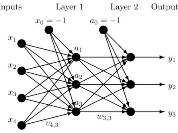
While we considereda priorithe more general case, it turned out that for our purposes an MLP with only two layers is sufficient. We shall denote bym,pandrthe number of inputs, hidden neurons and output neurons, respectively. Figure 1 illustrates the
:
>
XXXX XXz :
>
Z Z
Z Z
Z Z
~ XXXX
XXz :
\
\
\
\
\
\
\
\ Z
Z Z
Z Z
Z
~ XXXX
XXz
@
@
@ R A
A A
A A
A U B
B B
B B
B B
B BB N
H HH
HH H j
@
@
@
@
@
@ R -
* H -
HH H
HHj
* -
@
@
@ R A
A A
A A
A U B
B B
B B
B B
B BBN
-
-
- y
y y y
y y
y y y
y y y
Inputs Layer 1 Layer 2 Outputs
x1
x2
x3
x4
x0=−1
y1
y2
y3
v4,3 w3,3
a0=−1
a1
a2
a3
Figure 1: Structure of the MLP
general structure of a two-layered perceptron. The weight matricesV ∈R(m+1)×p and W ∈ R(p+1)×r are determined by the backpropagation algorithm of Rumelhart et al.
(1986). The trained two-layered perceptron gathers its knowledge in V and Wfrom the training set, which in our case are various sets of profiles of ballots with prespecified winners. For profiles without specification of a winner we then obtain the ‘choice’ of the trained neural network by determining first the activation level
hj :=
m
X
i=0
vijxi , aj :=g(hj) = 1
1 +e−βhj , (2.1)
for each hidden neuron, and subsequently the activation level ok :=
p
X
j=0
wjkaj , yk:=g(hk) = 1
1 +e−βhk , (2.2)
for each output neuron. For more detailed description and analysis of neural networks, see, e.g., Haykin (1999) and Marshland (2009).
3 Data generation
We considered cases with 7, 9 or 11 voters and 3, 4 or 5 alternatives. For instance, in the case of three alternatives each voter can have one of six different linear orderings, resulting in 67 = 279936 profiles for seven voters (if we neglect symmetries). In the case of three alternatives 1000 profiles and five neurons proved to be sufficient for the learning phase. These parameter values were also sufficient for verifying the unanimity principle with four and five alternatives. With four alternatives and eleven voters, the number of possible profiles increases to 2411 = 1521681143169024 ≈ 1.52∗1015. In order to keep the problem computationally tractable we took 3000 profiles with five
7If ties between two or more alternatives remain after the first round, they are broken according to some fixed exogenous tie breaking rule. For our purposes, a specification of such tie breaking rule is not necessary because we consider only small numbers of alternatives here. Note that due to our assumption of an odd number of voters, tie breaking is never an issue in the second round.
neurons and 10000 profiles with 15 neurons for the cases of four and five alternatives, respectively, in the training phase. For verifying the Pareto property, we took 10000 profiles with 15 neurons in case of four alternatives and 20000 profiles with 30 neurons in case of five alternatives.
We encoded preference orderings in the following way. Let X ={x1, x2, . . . , xq}.
If xi1 xi2 · · · xiq, where (i1, . . . , iq) is a permutation of (1, . . . , q), we store the respective pairwise comparisons in a vector corresponding to the upper triangular matrix (ajk)q,qj=1,k=j+1 with ajk = 1 if xj xk and ajk = 0 otherwise. For example, the orderingx1x4x2x3is coded by (1,1,1,1,0,0) corresponding to the binary comparisonsx1x2,x1x3, x1 x4, x2 x3, x2 x4,x3x4. A profile is then given by a row vector withn·q(q−1)/2 entries.
To generate a preference profile, we alternatively invoked the impartial culture (IC) and the anonymous impartial culture (AIC) assumption. In the former case, the selection of each preference profile is equally like, while in the latter case each anonymous preference profile is equally likely (for a detailed discussion of the IC vs. AIC assumptions, see Eˇgecioˇglu and Giritligil, 2013).8
To complete an input of a training set we also specified a target alternative, the
‘winner’ of the respective voting rule. For this we used the so-called ‘1-of-N encoding,’
i.e. alternativexi is represented by the indicator vector (0, . . . ,0,1,0, . . . ,0), in which theith coordinate equals 1 and all other entries are set to zero.
When testing unanimity we picked an alternative which served as the top alternative in each voter’s preference ordering. We then randomly ordered the other alternatives at the lower ranks in each voter’s ordering. The target value for a profile was its unanimous ‘top alternative.’ In case of the Pareto property we picked two alternatives xandyand randomly assigned them ranks in the voters’ orderings, making sure that y is belowxin each voter’s ordering. The other alternatives were randomly assigned.
We then tooky as the target value for the corresponding profile.9
When training for a winner or a set of winners, we considered five scenarios. First, we trained on the subset of profiles with a (necessarily unique) Condorcet winner from the randomly generated 1000, 3000, and 10000 profiles in case of three, four, and five alternatives, respectively; second, we trained on the subset of profiles with a unique Borda winner; third we trained on the subset of profiles with a unique plurality winner;
fourth, we trained on the subset of profiles on which the Condorcet winner was equal to the unique Borda winner; and fifth, we trained on the subset of profiles on which the Condorcet winner, the unique Borda winner and the unique plurality winner all coincided.
The generation of profiles and the training set was written in C#. We then employed Marshland’s (2009) MLP Python class to train the neural network and, subsequently, to ‘predict’ the winning alternative without specified target value. The prediction was carried out on an independent new random sample of 1000 profiles. The statistical evaluation was carried out in Excel. All program codes are available from the authors upon request.
8For both the IC and AIC cases, we also carried out the training based only on the ‘pairwise majority margin’ associated with profiles of ballots, i.e. for each pair of alternatives, the MLP was only given the information of how many voters preferred either alternative. While this generally leads to a loss of information it also yields a substantial reduction in the dimension of the input. The different representation of the input had no effect on the results.
9Since other dominance relationships could emerge in the profile, we made sure thatywas declared as target value only if it was the unique alternative that did not itself dominate another alternative.
For each combination of alternatives and voters, as well as for the five investigated sets of training profiles (altogether 45 cases), we generated five random training seeds in order to generate the training samples, and we took five random network seeds for the training procedure of the MLP. An alternative for a profile was counted as being selected by the five MLPs trained on the same sample (i.e. generated by the same training seed) if the same alternative was chosen by at least three out of the five possible network seeds (i.e. selected by the majority of trained MLPs on the same training seed). In case of non-existence of such an alternative the respective five MLPs failed to determine a winner and were counted as ‘indecisive.’ Only a low number of MLPs were indecisive in this sense (see Table 8 in Appendix A below). The learning rates for the five training seeds were thus determined, resulting in average learning rates for any combination of alternatives, voters, and set of winners. Altogether we have thus evaluated and aggregated 25 results for each of the 45 cases.
4 Testing unanimity and the Pareto property
The results for the unanimity principle are very straightforward. For all combinations of number of alternatives and number of voters, the trained neural network selected the unanimous top alternative with 100% accuracy, both for the IC and AIC cases.
Continuing with the impartial culture assumption (IC), in the case of three alter- natives the trained MLPs learned the Pareto dominated alternative on average with 99.54%, 99.66%, and 99.56% accuracy for 7, 9, and 11 voters, respectively. In case of four alternatives the Pareto dominated alternative was learned with 93.90%, 95.10%, and 95.68% accuracy for 7, 9, and 11 voters, respectively. However, to achieve this result we had to increase the training sample to 10000 and the number of hidden neu- rons to 15. The results became less satisfactory for the case of five alternatives for which we obtained respective learning ratios of 61.74%, 68.18%, and 73.24% even for training samples of size 20000 and 15 hidden neurons. By further increasing the num- ber of hidden neurons to 30 we could increase the respective learning rates to 67.60%, 79.20%, and 84.68%. However, the long training time (even on fast computers) makes it difficult to experiment with different numbers of hidden neurons and larger samples.
Evidently, the training sample size of 20000 profiles is extremely small compared to the huge number of possible profiles having a Pareto dominated alternative in the case of five alternatives (about 55.99 millions, 2.02 billions, 72.56 billions for 7, 9, and 11 voters, respectively). Using almost one week of computation time, we determined the learning rates for five training sets of size 50000 associated with the same training seed and five network seeds. We found that the average learning rate increased to 88.78%
(with five alternatives, 11 voters and 30 hidden neurons). Therefore, we conjecture that the Pareto property can be accurately learned by the MLP also for five alternatives, but a more precise verification of this claim lies beyond our computational capacities.
Turning to the anonymous impartial culture (AIC), we found that with three al- ternatives the MLP could learn the Pareto dominated alternative based on a training sample size of 1000 profiles and employing five hidden neurons with 99.38%, 97.80%, and 96.78% accuracy for 7, 9, and 11 voters, respectively. The corresponding values for the case of four alternatives and 15 hidden neurons were 89.94%, 91.70%, and 93.14%, respectively. Since we obtained similar (if a bit lower) values as under the IC hypothesis, we did not investigate the case of five alternatives for the AIC.
Summarizing, the MLP passed the unanimity test with perfect accuracy and the Pareto dominance test with a very high level of accuracy for three and four alternatives.
Furthermore, our results lend support to the conjecture that the Pareto property can also be learned at a high level of accuracy for five alternatives if the training sample size is sufficiently large.
5 Results: The social choices by the neural network
In this section, we present our results in detail for the IC case with binary encoding of preference profiles. The corresponding results for the AIC case as well as for the representation of the input in terms of pairwise majority margins can be found in Appendices B, C and D. While the precise values differ slightly, the general conclusion is that all results are robust with respect to the way the training samples are generated.
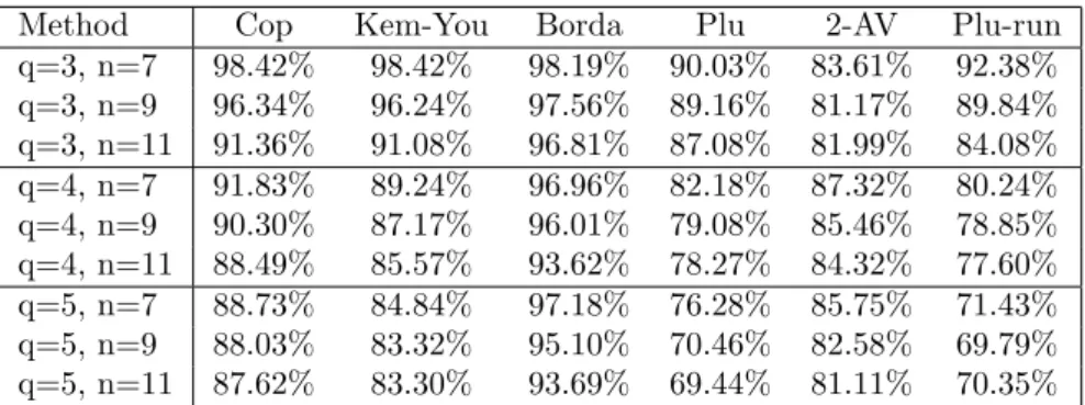
First, we consider the case in which we took profiles with a Condorcet winner as training sample and the Condorcet winner as target value. Table 1 shows the corresponding results for the cases of three, four, and five alternatives and 7, 9, and 11 voters, respectively. The table entries give the average percentages of those cases in which a trained MLP selects a winner of the method appearing in the respective column heading.10 As can be seen, the Borda count performs best with the only exception in the case of three alternatives and 7 voters. It is particularly remarkable that the Borda count outperforms both the Copeland and the Kem´eny-Young method even though these are Condorcet consistent while the Borda is not.
Method Cop Kem-You Borda Plu 2-AV Plu-run
q=3, n=7 98.42% 98.42% 98.19% 90.03% 83.61% 92.38%
q=3, n=9 96.34% 96.24% 97.56% 89.16% 81.17% 89.84%
q=3, n=11 91.36% 91.08% 96.81% 87.08% 81.99% 84.08%
q=4, n=7 91.83% 89.24% 96.96% 82.18% 87.32% 80.24%
q=4, n=9 90.30% 87.17% 96.01% 79.08% 85.46% 78.85%
q=4, n=11 88.49% 85.57% 93.62% 78.27% 84.32% 77.60%
q=5, n=7 88.73% 84.84% 97.18% 76.28% 85.75% 71.43%
q=5, n=9 88.03% 83.32% 95.10% 70.46% 82.58% 69.79%
q=5, n=11 87.62% 83.30% 93.69% 69.44% 81.11% 70.35%
Table 1: Trained on Condorcet winners
While the two Condorcet consistent methods are also not far from MLPs choices (with a slight advantage of the Copeland method as compared to the Kem´eny-Young method), the other methods differ significantly, in particular for more alternatives.
Interestingly, and in contrast to the two versions of plurality rule, coincidence of MLPs choice with the 2-approval voting winner is larger for four and five alternatives than for three.11
10The separating line between the cases of three, four, and five alternatives is to emphasize that the training set size is increasing in the number of alternatives.
11In evaluating the differences in percentages one should keep in mind that on many profiles different methods agree, so that even small differences in percentage points may hint at significant underlying differences in learning performance.
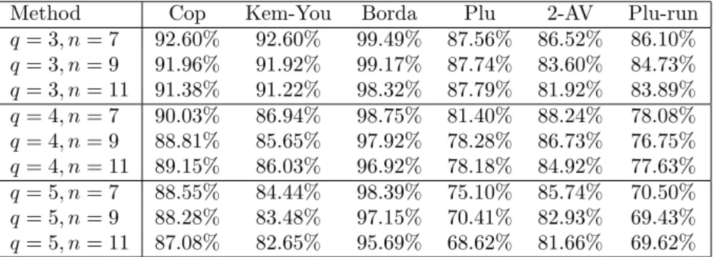
We obtain essentially the same ordering of methods in terms of coincidence with MLPs choices if we train the neural network either (i) on a unique Borda winner (see Table 2), or (ii) on a unique plurality winner (see Table 3). The Borda count still performs best among all voting methods. Not surprisingly, MLPs choice behavior comes even closer to the Borda count if trained to choose the Borda winner. On the other hand, it is remarkable that in the case of three alternatives plurality rule does not seem to perform better even when the MLP is trained to choose the plurality winner (compare the first three entries in the column for plurality rule across Tables 1-3).
Method Cop Kem-You Borda Plu 2-AV Plu-run
q= 3, n= 7 92.60% 92.60% 99.49% 87.56% 86.52% 86.10%
q= 3, n= 9 91.96% 91.92% 99.17% 87.74% 83.60% 84.73%
q= 3, n= 11 91.38% 91.22% 98.32% 87.79% 81.92% 83.89%
q= 4, n= 7 90.03% 86.94% 98.75% 81.40% 88.24% 78.08%
q= 4, n= 9 88.81% 85.65% 97.92% 78.28% 86.73% 76.75%
q= 4, n= 11 89.15% 86.03% 96.92% 78.18% 84.92% 77.63%
q= 5, n= 7 88.55% 84.44% 98.39% 75.10% 85.74% 70.50%
q= 5, n= 9 88.28% 83.48% 97.15% 70.41% 82.93% 69.43%
q= 5, n= 11 87.08% 82.65% 95.69% 68.62% 81.66% 69.62%
Table 2: Trained on Borda winners
Method Cop Kem-You Borda Plu 2-AV Plu-run
q= 3, n= 7 91.80% 91.78% 97.35% 87.38% 86.13% 85.98%
q= 3, n= 9 90.08% 89.92% 95.96% 87.33% 83.29% 84.25%
q= 3, n= 11 88.88% 88.32% 93.28% 85.76% 81.19% 82.15%
q= 4, n= 7 89.93% 87.67% 96.41% 82.31% 88.55% 79.53%
q= 4, n= 9 87.73% 85.11% 93.31% 79.32% 85.98% 77.96%
q= 4, n= 11 86.73% 84.12% 91.12% 78.89% 84.57% 77.75%
q= 5, n= 7 89.42% 86.17% 97.06% 78.52% 87.30% 74.22%
q= 5, n= 9 89.75% 86.22% 95.81% 75.17% 86.81% 75.51%
q= 5, n= 11 89.32% 85.94% 94.44% 72.29% 85.40% 74.10%
Table 3: Trained on plurality winners
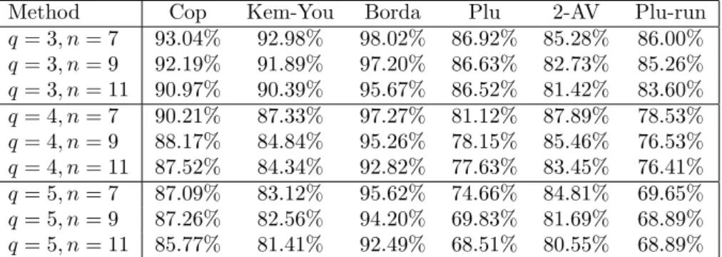
In order to give the Condorcet consistent methods (Copeland and Kem´eny-Young) and the Borda count exactly the samea prioricondition in the learning phase, we also took as the training sample the subset of those profiles with identical Condorcet and (unique) Borda winner. The results are shown in Table 4. As can be inferred from the numbers, the main conclusions drawn above do not change. In particular, the behavior of the trained MLP still mimics most closely that of the Borda count.
Taking the analysis one step further, we finally trained the MLP on the subset of those profiles on which the Condorcet winner, the unique Borda winner and the unique plurality winner all coincided. The results, shown in Table 5, confirm all conclusions from above. In particular, both plurality and plurality with runoff still perform signifi- cantly worse than either the Condorcet consistent methods and the Borda count, with
Method Cop Kem-You Borda Plu 2-AV Plu-run q= 3, n= 7 93.04% 92.98% 98.02% 86.92% 85.28% 86.00%
q= 3, n= 9 92.19% 91.89% 97.20% 86.63% 82.73% 85.26%
q= 3, n= 11 90.97% 90.39% 95.67% 86.52% 81.42% 83.60%
q= 4, n= 7 90.21% 87.33% 97.27% 81.12% 87.89% 78.53%
q= 4, n= 9 88.17% 84.84% 95.26% 78.15% 85.46% 76.53%
q= 4, n= 11 87.52% 84.34% 92.82% 77.63% 83.45% 76.41%
q= 5, n= 7 87.09% 83.12% 95.62% 74.66% 84.81% 69.65%
q= 5, n= 9 87.26% 82.56% 94.20% 69.83% 81.69% 68.89%
q= 5, n= 11 85.77% 81.41% 92.49% 68.51% 80.55% 68.89%
Table 4: Trained on joint Borda and Condorcet winners the latter taking the clear lead again.
Method Cop Kem-You Borda Plu 2-AV Plu-run
q= 3, n= 7 92.61% 92.49% 97.32% 86.71% 85.26% 85.49%
q= 3, n= 9 91.37% 91.01% 96.15% 86.62% 82.39% 84.65%
q= 3, n= 11 88.80% 87.82% 92.60% 85.26% 79.99% 81.91%
q= 4, n= 7 88.59% 85.68% 94.78% 80.35% 87.26% 77.63%
q= 4, n= 9 86.36% 83.24% 91.72% 76.89% 84.18% 74.82%
q= 4, n= 11 84.90% 81.56% 88.98% 76.55% 82.31% 74.43%
q= 5, n= 7 86.14% 82.27% 93.03% 74.19% 83.93% 69.40%
q= 5, n= 9 85.76% 81.12% 92.01% 69.35% 81.10% 68.04%
q= 5, n= 11 84.48% 80.27% 90.08% 67.95% 80.04% 68.30%
Table 5: Trained on joint Borda, Condorcet and plurality winners
It is worth mentioning that the great majority of percentages in Tables 1-5 is de- creasing both in the number of alternatives and in the number of voters for all inves- tigated voting rules. However, this does not necessarily mean that the MLP learns these rules with lower accuracy for higher number of alternatives and voters. Indeed, the increase in the size and dimension of the potential input data has not been ac- counted for when we increased the number of voters, and only partially offset by the increase in the training sample size when we increased the number of alternatives. For instance, for q= 3 and n= 7 the dimension of the input (under binary encoding) is n·q(q−1)/2 = 21 while it grows to 66 as we move to the case q= 4 andn= 11. We decided to use fixed sample sizes for more voters in order to reduce computing time.
As can be seen from the figures in the tables, the qualitative results are not affected.
6 Concluding remarks
Our results show that – in onesense – Borda’s count is the mostsalient of a number of popular voting methods: it is the voting rule that best describes the behavior of a trained neural network in a voting environment. One should be careful, however, in using this finding as an argument for the general superiority of the Borda count
vis-`a-vis other voting rules, even the ones tested here. Indeed, our results may ‘only’
show that the internal topology of the employed MLP is best adapted to the ‘linear’
mathematical structure underlying the Borda rule. But then again, if this common underlying structure is successful in a number of different application areas, the Borda count must at least be considered as a serious contender in the competition for ‘optimal’
voting rule.
One may interpret learning by neural networks also as a device to select a ‘suitable’
degree of complexity. On such an account, plurality rule and its variants (plurality with runoff and 2-approval) turn out to be too simple while the two investigated Condorcet consistent methods seem to be too sophisticated. When choosing a winner, the MLP obviously uses more information than only the top ranked alternatives in each ballot.
On the other hand, it does also not seem to make the pairwise comparisons necessary in order to determine the Copeland or Kem´eny-Young winners. The comparison of the learning rates of the Copeland method vis--vis the Kem´eny-Young method is well in line with this interpretation: the computationally more complex of these two methods, the Kem´eny-Young rule, performs consistently worse.
Based on our analysis one might conjecture that the intuitive choices of humans not trained in social choice theory would also be more in line with Borda’s count than with any other voting method. However, this has to be confirmed by further well-designed experiments with human subjects.
References
[1] Arrow, K. J.1951/63, Social Choice and Individual Values(First edition: 1951, second edition: 1963), Wiley, New York.
[2] Balinski, M. and R. Laraki (2016), Majority judgement vs. majority rule, preprint, https://hal.archives-ouvertes.fr/hal-01304043.
[3] Dorsey, R.E., J.D. Johnsonand M.V. van Boening(1994), The use of ar- tificial neural networks for estimation of decision surfaces in first price sealed bid auctions, in W.W. Cooper and A.B. Whinston (eds.),New decisions in computa- tional economics, 19-40, Kluwer Academic Publishing, Dordrecht.
[4] Drton, M., G. H¨agele, D. Haneberg, F. PukelsheimandW. Reif(2004), A rediscovered Llull tract and the Augsburg Web Edition of Llull’s electoral writ- ings,Le M´edi´eviste et l’ordinateur,43, http://lemo.irht.cnrs.fr/43/43-06.htm.
[5] Eˇgecioˇglu, ¨O. and A.E. Giritligil (2013), The Impartial, Anonymous, and Neutral Culture Model: A Probability Model for Sampling Public Preference Structures,Journal of Mathematical Sociology37, 203-222.
[6] Elkind, E.,P. FaliszewskiandA. Slinko(2015), Distance rationalization of voting rules,Social Choice and Welfare45, 345-377.
[7] Fishburn, P.C. (1978), Axioms for approval voting: direct proof, Journal of Economic Theory19, 180-185, corrigendum45(1988) 212.
[8] Giritligil Kara, A.E. andM.R. Sertel (2005), Does majoritarian approval matter in selecting a social choice rule? An exploratory panel study,Social Choice and Welfare25, 43-73.
[9] Goodin, R.E.andC. List(2006), A conditional defense of plurality rule: Gener- alizing May’s theorem in a restricted informational environment,American Jour- nal of Political Science50, 940-949.
[10] H¨agele, G. and F. Pukelsheim (2008), The electoral systems of Nicholas of Cusa in theCatholic Concordanceand beyond, in: G. Christianson, T.M. Izbicki and C.M. Bellitto (eds.),The church, the councils, and reform – The legacy of the Fifteenth Century, Catholic University of America Press, Washington D.C.
[11] Haykin, S.(1999),Neural Networks: A Comprehensive Foundation, 2nd Edition, Prentice-Hall.
[12] Henriet, D.(1985), The Copeland choice function: an axiomatic characteriza- tion,Social Choice and Welfare2, 49-63.
[13] Laslier, J.F.(2011), And the loser is ... plurality voting, in: D.S. Felsenthal and M. Machover (eds.),Electoral systems – Paradoxes, assumptions, and procedures, Springer, Heidelberg.
[14] Leshno, M.,D. MollerandP. Ein-Dor(2002), Neural nets in a group decision process,International Journal of Game Theory31, 447-467.
[15] Marshland, S. (2009), Machine Learning: An Algorithmic Perspective, Chap- man & Hall, CRC Press, Boca Raton, Florida, USA.
[16] McLean, I.andA. Urken(1995),Classics of social choice, University of Michi- gan Press, Ann Arbor.
[17] McNelis, P.D.(2005),Neural Networks in Finance, Academic Press, Boston.
[18] Nehring, K. and M. Pivato (2011), Majority rule in the absence of a ma- jority, preprint, http://www.parisschoolofeconomics.eu/docs/ydepot/semin/texte 1112/KLA2012MAJ.pdf.
[19] Procaccia, A.D., A. Zohar, Y. Pelegand J.S. Rosenschein (2009), The learnability of voting rules,Artificial Intelligence 173, 1133-1149.
[20] Pukelsheim, F. (2003), Social choice: The historical record, in: S. Garfunkel, Consortium for Mathematics and its applications (eds.),For all practical purposes – Mathematical literacy in today’s world (sixth edition), Freeman, New York.
[21] Richards, W., H.S. Seung and G. Pickard (2006), Neural voting machine, Neural Networks19, 1161-1167.
[22] Risse, M.(2005), Why the count de Borda cannot beat the Marquis de Condorcet, Social Choice and Welfare25, 95-113.
[23] Rumelhart, D.E.,G.E. HintonandR.J. Williams(1986), Learning Internal Representations by Error Propagation, in: D.E. Rumelhart, J.L. McClelland, and the PDP research group (eds.),Parallel distributed processing: Explorations in the microstructure of cognition, Volume 1: Foundations. MIT Press, Cambridge MA.
[24] Sgroi, D.andZizzo, D.J.(2009): Learning to play 3×3 games: Neural networks as bounded-rational players, Journal of Economic Behavior & Organization 69, 27-38.
[25] Silver, D., A. Huang, C. J. Maddison, A. Guez, L. Sifre, G. van den Driessche, J. Schrittwieser, I. Antonoglou, V. Panneershelvam, M. Lanctot, S. Dieleman, D. Grewe, J. Nham, N. Kalchbrenner, I. Sutskever, T. Lillicrap, M. Leach, K. Kavukcuoglu, T. Graepel, and D. Hassabis(2016), Mastering the game of Go with deep neural networks and tree search,Nature529, 484-489.
[26] Saari, D.G. (2000), Mathematical structure of voting paradoxes II: Positional voting,Economic Theory15, 55-101.
[27] Smith, J.H.(1973), Aggregation of preferences with variable electorate, Econo- metrica41, 1027-1041.
[28] Young, H.P. (1974), An axiomatization of Borda’s rule, Journal of Economic Theory9, 43-52.
[29] Young, H.P.(1975), Social choice scarring rules,SIAM Journal of Applied Math- ematics28, 824-838.
[30] Young, H.P.andA. Levenglick(1978), A consistent extension of Condorcet’s election principle,SIAM Journal on Applied Mathematics35, 285-300.
Appendix: Robustness
In this appendix, we check our results for robustness. In Appendix A, we report additional results for the IC case with binary encoding of the input profiles. The subsequent appendices then contain results for the AIC case and/or the case in which training was carried out with a representation of the input in terms of majority margins.
Appendix A. Additional results for IC with binary encoding
In those cases in which we trained the MLP on the set of profiles having a Condorcet winner or a unique Borda winner, we also separately investigated the trained MLPs’
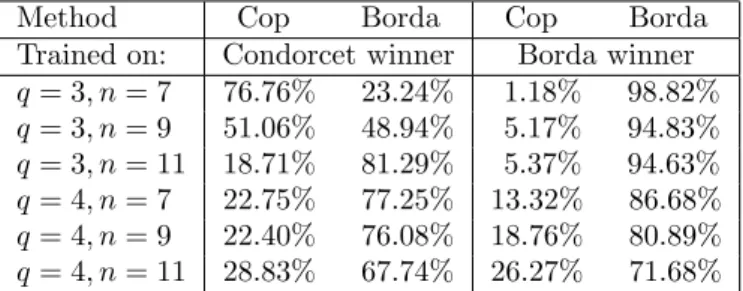
choices on the subset of those profiles on which the Condorcet winner differed from the unique Borda winner. Out of the 1000 profiles we had about 20 to 60 profiles of this kind, depending on the values ofqandn. Although the number of such profiles is small, our results are meaningful because we have investigated all the 25 generated input files with 1000 profiles for eachq∈ {3,4}andn∈ {7,9,11}. The second and third columns of Table 6 show the percentages of cases in which the Copeland winner and the Borda winner was chosen, respectively, when the MLP was trained on the set of profiles with Condorcet winners. We see that even for these profiles the Borda winner was chosen more frequently, with the exception of the cases q = 3 and n∈ {7,9}; and even for these two cases the percentages for the Borda winner is significant. In the fourth and fifth columns we see the same percentages when the MLP was trained on the set of profiles with unique Borda winners. In the latter case the MLP unambiguously favors the Borda winner (however, the advantage in favor of the Borda count is decreasing in the number of voters and alternatives).
Method Cop Borda Cop Borda
Trained on: Condorcet winner Borda winner q= 3, n= 7 76.76% 23.24% 1.18% 98.82%
q= 3, n= 9 51.06% 48.94% 5.17% 94.83%
q= 3, n= 11 18.71% 81.29% 5.37% 94.63%
q= 4, n= 7 22.75% 77.25% 13.32% 86.68%
q= 4, n= 9 22.40% 76.08% 18.76% 80.89%
q= 4, n= 11 28.83% 67.74% 26.27% 71.68%
Table 6: Results only on profiles with Condorcet winner6= unique Borda winner The investigated voting methods differ in how often they select a unique winner which might cause a bias in the results. In Table 7 we gathered the averages on how frequently a method does not have a unique winner. We can observe that for more alternatives and also for more voters the Borda count becomes relatively more decisive in the sense that it specifies a unique winner more often than the other rules (with the exception of plurality with runoff). In principle, this could affect the learning ratios. However, the results reported in Section 5 do not display significant differences in the comparison of voting rules across different numbers of alternatives. This can be interpreted as evidence that our results are robust to the way ties are treated.12
12It is worth mentioning that plurality rule does not benefit in terms of learning ratios from its significantly high percentage of ties (cf. the results in Tables 1-5).
Nevertheless, below in Tables 9 and 10 we analyze the performance of the different voting rules on the subset of those profiles on which no ties occur.
Method Cop Kem-You Borda Plu 2-AV Plu-run
q= 3, n= 7 7.20% 6.84% 13.44% 18.84% 35.26% 1.96%
q= 3, n= 9 8.24% 7.32% 12.76% 18.12% 21.44% 7.72%
q= 3, n= 11 8.26% 6.84% 10.82% 24.52% 19.18% 0.88%
q= 4, n= 7 14.08% 14.38% 14.36% 24.96% 31.48% 9.82%
q= 4, n= 9 14.74% 13.90% 13.02% 27.38% 27.92% 2.74%
q= 4, n= 11 15.32% 14.72% 10.92% 22.30% 25.00% 6.42%
q= 5, n= 7 18.10% 22.42% 12.12% 37.78% 30.98% 10.14%
q= 5, n= 9 19.70% 22.82% 11.44% 27.30% 27.68% 5.80%
q= 5, n= 11 19.18% 21.10% 10.50% 32,08% 26.16% 6.60%
Table 7: How frequently does a method not have a unique winner?
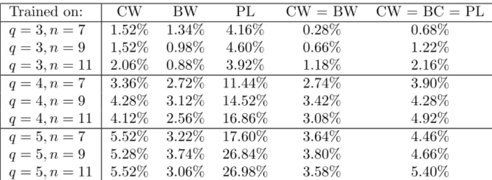
It is important to note that the MLP itself does not always give us an answer, i.e. for some profiles the trained MLP is indecisive and does not specify an alternative as target value. This is not surprising since the rules used to train the MLP themselves do not always give a unique answer. Comparing Table 7 and Table 8, we see that the trained MLP in fact gives an (unique) answer for far more profiles than the respective voting rules (CW, BW and PL stand for Condorcet winner, Borda winner, and plurality winner, respectively).
Trained on: CW BW PL CW = BW CW = BC = PL
q= 3, n= 7 1.52% 1.34% 4.16% 0.28% 0.68%
q= 3, n= 9 1,52% 0.98% 4.60% 0.66% 1.22%
q= 3, n= 11 2.06% 0.88% 3.92% 1.18% 2.16%
q= 4, n= 7 3.36% 2.72% 11.44% 2.74% 3.90%
q= 4, n= 9 4.28% 3.12% 14.52% 3.42% 4.28%
q= 4, n= 11 4.12% 2.56% 16.86% 3.08% 4.92%
q= 5, n= 7 5.52% 3.22% 17.60% 3.64% 4.46%
q= 5, n= 9 5.28% 3.74% 26.84% 3.80% 4.66%
q= 5, n= 11 5.52% 3.06% 26.98% 3.58% 5.40%
Table 8: How frequently does MLP not give us an answer?
In Tables 9 and 10 we restrict ourselves to those cases in which (i) the trained MLP was decisive and (ii) the respective voting rule displays no ties (in any rank).
We determined how frequently the MLP chose the first-ranked alternative, the second- ranked alternative, and so on, according to the method appearing in the tables’ column headings, respectively. In Table 9, we consider again the case in which the MLP was trained on the Condorcet winner. With the exception of the case of three alternatives and 7 voters the first-ranked alternative according to the Borda count was chosen most frequently by the trained MLP. Lower ranked alternatives are rarely chosen by the MLP.13 When training on the unique Borda winner, the performance of the Borda count increases while the other qualitative results remain in tact (see Table 10).
13Remarkably, among the losers of the respective rules the plurality looser is chosen more frequently than the losers of other methods.
Rank Cop Kem-You Borda Plu 2-AV Plu-run 1st 98.32% 98.33% 97.94% 88.15% 78.70% 93.38%
q=3, n=7 2nd 1.68 % 1.67% 2.06% 11.80% 21.30% 4.28%
3rd 0.00% 0.00% 0.00% 0.05% 0.00% 3.35%
1st 96.07% 96.00% 97.23% 86.86% 76.07% 89.84%
q=3, n=9 2nd 3.93% 4.00% 2.77% 10.32% 21.97% 6.59%
3rd 0.00% 0.00% 0.00% 2.82% 1.96% 3.38%
1st 90.68% 90.52% 96.45% 86.39% 77.99% 84.08%
q=3, n=11 2nd 9.28% 9.37% 3.43% 12.81% 21.53% 11.37%
3rd 0.04% 0.11% 0.11% 0.80% 0.48% 4.55%
1st 91.06% 87.73% 96.66% 78.47% 84.58% 80.24%
q=4, n=7 2nd 8.76% 11.89% 3.34% 16.77% 14.82% 10.86%
3rd 0.19% 0.33% 0.00% 4.52% 0.59% 8.90%
4th 0.00% 0.05% 0.00% 0.25% 0.00%
1st 89.35% 85.58% 95.64% 77.51% 82.93% 78.85%
q=4, n=9 2nd 10.41% 13.92% 4.32% 20.55% 15.70% 12.19%
3rd 0.24% 0.50% 0.05% 1.43% 1.34% 8.96%
4th 0.00% 0.00% 0.00% 0.52% 0.03%
1st 87.43% 83.84% 93.24% 74.56% 81.84% 77.60%
q=4, n=11 2nd 12.19% 15.10% 6.55% 19.48% 16.70% 13.24%
3rd 0.39% 0.90% 0.18% 5.37% 1.14% 9.16%
4th 0.10% 0.17% 0.02% 0.59% 0.22%
1st 87.37% 82.20% 97.02% 74.60% 82.17% 71.43%
2nd 12.25% 16.50% 2.98% 18.44% 16.55% 12.23%
q=5, n=7 3rd 0.38% 1.05% 0.00% 5.93% 0.18% 16.35%
4th 0.00% 0.24% 0.00% 0.30% 1.09%
5th 0.00% 0.00% 0.00% 0.73% 0.00%
1st 86.44% 80.94% 94.81% 65.49% 78.87% 69.79%
2nd 12.48% 17.01% 5.07% 26.47% 18.73% 13.56%
q=5, n=9 3rd 1.08% 1.95% 0.12% 2.83% 1.53% 16.65%
4th 0.00% 0.11% 0.00% 4.83% 0.70%
5th 0.00% 0.00% 0.00% 0.37% 0.17%
1st 86.17% 81.35% 93.40% 65.51% 77.98% 70.35%
2nd 12.81% 16.57% 6.15% 26.48% 18.24% 13.08%
q=5, n=11 3rd 0.92% 1.79% 0.39% 5.16% 3.01% 16.57%
4th 0.03% 0.27% 0.02% 2.32% 0.51%
5th 0.04% 0.03% 0.02% 0.53% 0.25%
Table 9: Rank of MLP’s choice according to different rules if trained on CW
Rank Cop Kem-You Borda Plu 2-AV Plu-run 1st 92.13% 92.16% 99.42% 85.24% 83.13% 86.10%
q= 3, n= 7 2nd 7.87 % 7.84% 0.58% 14.66% 16.87% 10.12%
3rd 0.00% 0.00% 0.00% 0.10% 0.00% 3.77%
1st 91.32% 91.36% 99.06% 85.10% 79.11% 84.73%
q= 3, n= 9 2nd 8.68% 8.64% 0.94% 11.75% 19.26% 11.41%
3rd 0.00% 0.00% 0.00% 3.16% 1.62% 3.87%
1st 90.66% 90.63% 98.14% 87.19% 78.00% 83.89%
q= 3, n= 11 2nd 9.34% 9.37% 1.86% 12.23% 21.58% 11.99%
3rd 0.00% 0.00% 0.00% 0.58% 0.42% 4.11%
1st 88.82% 85.01% 98.59% 77.17% 85.58% 78.08%
q= 4, n= 7 2nd 10.95% 14.72% 1.41% 18.24% 13.82% 13.18%
3rd 0.24% 0.24% 0.00% 4.37% 0.60% 8.74%
4th 0.00% 0.02% 0.00% 0.22% 0.00%
1st 87.55% 83.66% 97.74% 76.48% 84.41% 76.75%
q= 4, n= 9 2nd 12.09% 15.75% 2.22% 21.28% 14.30% 13.87%
3rd 0.36% 0.55% 0.05% 1.75% 1.27% 9.38%
4th 0.00% 0.05% 0.00% 0.48% 0.03%
1st 87.74% 83.98% 96.61% 74.38% 82.34% 77.63%
q= 4, n= 11 2nd 11.86% 15.40% 3.39% 19.70% 16.19% 13.34%
3rd 0.41% 0.60% 0.00% 5.32% 1.39% 9.03%
4th 0.00% 0.02% 0.00% 0.61% 0.08%
1st 87.23% 81.55% 98.25% 73.00% 81.91% 70.50%
2nd 12.14% 16.91% 1.71% 19.42% 16.64% 12.50%
q= 5, n= 7 3rd 0.63% 1.33% 0.05% 6.32% 0.33% 17.00%
4th 0.00% 0.21% 0.00% 0.39% 1.13%
5th 0.00% 0.00% 0.00% 0.86% 0.00%
1st 86.59% 81.29% 96.96% 65.62% 79.24% 69.43%
2nd 12.64% 16.94% 2.92% 26.33% 18.39% 13.64%
q= 5, n= 9 3rd 0.77% 1.61% 0.11% 2.87% 1.57% 16.93%
4th 0.00% 0.16% 0.00% 4.75% 0.69%
5th 0.00% 0.00% 0.00% 0.42% 0.11%
1st 85.49% 80.30% 95.44% 64.61% 78.86% 69.62%
2nd 13.45% 17.38% 4.27% 27.31% 17.87% 13.65%
q= 5, n= 11 3rd 1.04% 2.14% 0.27% 5.35% 2.66% 16.74%
4th 0.00% 0.16% 0.00% 2.15% 0.47%
5th 0.02% 0.03% 0.02% 0.58% 0.14%
Table 10: Rank of MLP’s choice according to different rules if trained on BW
Appendix B. Results under AIC with binary encoding
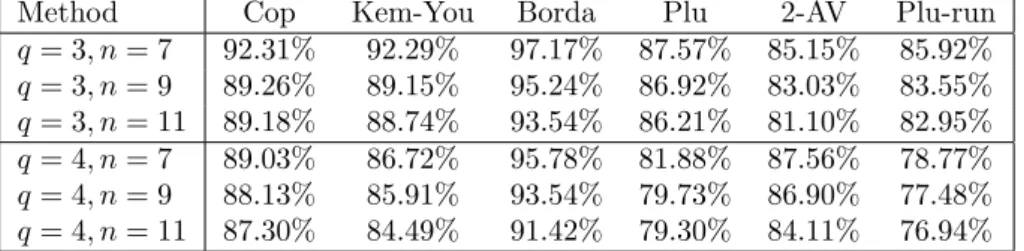
To confirm that our results are robust with respect to the distributional assumption underlying our sampling of preference profiles, we carried out (most of) the calculations described in the main part of the paper also for the anonymous impartial culture (AIC) hypothesis described in Section 3. Because of the large running time we limited ourselves to the cases of three and four alternatives. For q = 3 and q = 4 we again used a training set consisting of 1000 and 3000 profiles, respectively. If we compare Tables 1-5 of Section 5 with the corresponding Tables 11-15 below, we can observe the same qualitative results in terms of the ranking of voting rules. The percentages by which a neural network chooses an outcome according to a specific voting rule are almost identical for the IC and AIC cases even if they are on average slightly lower by approximately 0.13% points for the AIC cases.
Method Cop Kem-You Borda Plu 2-AV Plu-run
q=3, n=7 96.42% 96.42% 98.82% 88.14% 84.88% 89.07%
q=3, n=9 93.73% 93.69% 97.97% 87.30% 83.30% 86.99%
q=3, n=11 91.82% 91.63% 96.59% 87.40% 81.99% 84.57%
q=4, n=7 91.54% 88.78% 97.53% 81.07% 87.32% 78.44%
q=4, n=9 90.48% 87.77% 95.61% 79.26% 85.76% 77.96%
q=4, n=11 89.25% 85.89% 93.74% 78.06% 84.40% 76.82%
Table 11: Trained on Condorcet winners (AIC)
Method Cop Kem-You Borda Plu 2-AV Plu-run
q= 3, n= 7 92.71% 92.71% 99.76% 86.90% 86.48% 85.44%
q= 3, n= 9 92.06% 92.00% 99.15% 86.85% 84.40% 84.98%
q= 3, n= 11 91.59% 91.40% 98.14% 87.29% 82.38% 84.16%
q= 4, n= 7 89.98% 87.01% 98.48% 80.32% 87.47% 76.96%
q= 4, n= 9 89.47% 86.78% 97.41% 78.76% 86.76% 77.09%
q= 4, n= 11 89.15% 85.89% 96.80% 77.77% 85.46% 75.92%
Table 12: Trained on Borda winners (AIC)
Method Cop Kem-You Borda Plu 2-AV Plu-run
q= 3, n= 7 92.31% 92.29% 97.17% 87.57% 85.15% 85.92%
q= 3, n= 9 89.26% 89.15% 95.24% 86.92% 83.03% 83.55%
q= 3, n= 11 89.18% 88.74% 93.54% 86.21% 81.10% 82.95%
q= 4, n= 7 89.03% 86.72% 95.78% 81.88% 87.56% 78.77%
q= 4, n= 9 88.13% 85.91% 93.54% 79.73% 86.90% 77.48%
q= 4, n= 11 87.30% 84.49% 91.42% 79.30% 84.11% 76.94%
Table 13: Trained on plurality winners (AIC)
Method Cop Kem-You Borda Plu 2-AV Plu-run q= 3, n= 7 93.05% 92.93% 98.12% 86.38% 85.04% 85.36%
q= 3, n= 9 92.16% 91.84% 97.16% 86.47% 83.38% 85.36%
q= 3, n= 11 91.86% 91.23% 96.33% 86.63% 81.93% 84.28%
q= 4, n= 7 89.57% 86.58% 96.52% 80.13% 87.06% 76.93%
q= 4, n= 9 88.53% 85.61% 95.51% 78.47% 85.73% 76.18%
q= 4, n= 11 87.85% 84.31% 92.98% 77.15% 84.12% 75.37%
Table 14: Trained on joint Borda and Condorcet winners (AIC)
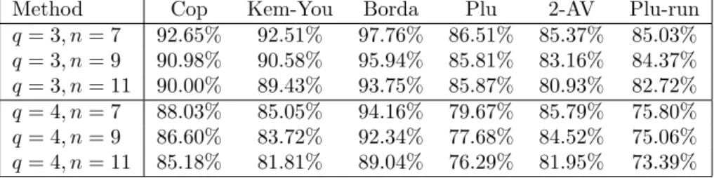
Method Cop Kem-You Borda Plu 2-AV Plu-run
q= 3, n= 7 92.65% 92.51% 97.76% 86.51% 85.37% 85.03%
q= 3, n= 9 90.98% 90.58% 95.94% 85.81% 83.16% 84.37%
q= 3, n= 11 90.00% 89.43% 93.75% 85.87% 80.93% 82.72%
q= 4, n= 7 88.03% 85.05% 94.16% 79.67% 85.79% 75.80%
q= 4, n= 9 86.60% 83.72% 92.34% 77.68% 84.52% 75.06%
q= 4, n= 11 85.18% 81.81% 89.04% 76.29% 81.95% 73.39%
Table 15: Trained on joint Borda, Condorcet and plurality winners (AIC)
Appendix C. Results under IC using the majority margin rep- resentation of profiles of ballots
The results of this appendix show that the way how profiles of ballots were represented does not affect our main conclusions. As described in the main text, we determined the pairwise majority margins corresponding to the generated preference profiles and used them as inputs to train the MLP. We carried out the calculations described in the main text using this representation of ballot profiles under the IC hypothesis. In order to check the robustness of our main results we limited ourselves to the cases of three and four alternatives using a training set consisting of 1000 profiles for both cases. If we compare the Tables 1-5 of Section 5 with the corresponding Tables 16-20, we again observe qualitatively the same results. In fact, the results under the majority margin representation favor the Borda rule even more strongly; in some cases we even obtained learning rates of 100%, i.e. perfect coincidence of MLP’s choices with the Borda count.
On average, the learning rates were by about 2.3% points higher than with binary encoding.
Appendix D. Results under AIC the majority margin represen- tation of profiles of ballots
This appendix shows the same results as the previous appendix for the AIC sampling (see Tables 21-25). Again, all qualitative conclusion remain valid.
Method Cop Kem-You Borda Plu 2-AV Plu-run q=3, n=7 97.55% 97.55% 99.81% 90.57% 85.28% 91.88%
q=3, n=9 95.43% 95.33% 99.69% 89.56% 82.94% 88.90%
q=3, n=11 93.98% 93.87% 99.98% 89.14% 82.62% 86.99%
q=4, n=7 92.34% 89.40% 99.38% 81.97% 89.15% 80.02%
q=4, n=9 90.50% 87.29% 99.44% 79.11% 87.87% 78.80%
q=4, n=11 91.20% 88.57% 99.62% 79.68% 86.40% 79.39%
Table 16: Trained on Condorcet winners (IC and majority margins)
Method Cop Kem-You Borda Plu 2-AV Plu-run
q= 3, n= 7 93.71% 93.71% 100.00% 89.23% 87.00% 88.74%
q= 3, n= 9 92.56% 92.52% 100.00% 89.08% 83.88% 86.34%
q= 3, n= 11 92.73% 92.61% 99.98% 88.88% 83.05% 86.00%
q= 4, n= 7 91.10% 88.01% 99.90% 81.60% 89.04% 78.94%
q= 4, n= 9 90.05% 86.81% 99.88% 79.14% 87.51% 78.58%
q= 4, n= 11 90.41% 87.53% 99.69% 79.16% 86.01% 78.34%
Table 17: Trained on Borda winners (IC and majority margins)
Method Cop Kem-You Borda Plu 2-AV Plu-run
q= 3, n= 7 93.90% 93.90% 99.92% 89.48% 87.21% 89.00%
q= 3, n= 9 93.85% 93.83% 99.94% 89.47% 84.24% 87.48%
q= 3, n= 11 92.49% 92.32% 99.98% 89.31% 83.25% 85.78%
q= 4, n= 7 92.58% 90.28% 99.47% 83.67% 90.88% 81.99%
q= 4, n= 9 91.13% 88.90% 99.44% 81.33% 89.65% 81.49%
q= 4, n= 11 91.70% 89.49% 99.62% 81.20% 88.75% 82.11%
Table 18: Trained on plurality winners (IC and majority margins)
Method Cop Kem-You Borda Plu 2-AV Plu-run
q= 3, n= 7 93.78% 93.78% 100.00% 89.32% 86.91% 88.60%
q= 3, n= 9 92.87% 92.85% 100.00% 88.86% 84.02% 86.42%
q= 3, n= 11 92.34% 92.22% 100.00% 89.00% 83.04% 85.94%
q= 4, n= 7 91.67% 88.68% 99.86% 82.26% 88.93% 79.55%
q= 4, n= 9 90.47% 87.14% 99.75% 79.05% 87.78% 77.94%
q= 4, n= 11 90.60% 87.75% 99.77% 78.80% 86.32% 78.68%
Table 19: Trained on joint Borda and Condorcet winners (IC and majority margins)
Method Cop Kem-You Borda Plu 2-AV Plu-run q= 3, n= 7 92.97% 92.97% 100.00% 89.21% 87.02% 87.99%
q= 3, n= 9 93.10% 93.06% 99.98% 88.59% 84.22% 86.69%
q= 3, n= 11 92.89% 92.77% 99.96% 89.03% 82.88% 86.29%
q= 4, n= 7 91.62% 88.86% 99.85% 81.93% 88.79% 79.54%
q= 4, n= 9 90.04% 86.79% 99.60% 79.12% 87.24% 78.08%
q= 4, n= 11 90.87% 87.89% 99.71% 79.67% 86.01% 79.13%
Table 20: Trained on joint Borda, Condorcet and plurality winners (IC and majority margins)
Method Cop Kem-You Borda Plu 2-AV Plu-run
q=3, n=7 97.22% 97.22% 99.73% 89.34% 85.66% 90.69%
q=3, n=9 95.49% 95.49% 99.98% 88.74% 83.91% 89.31%
q=3, n=11 94.65% 94.59% 99.69% 88.56% 83.15% 87.70%
q=4, n=7 92.07% 89.34% 99.52% 81.51% 88.27% 79.03%
q=4, n=9 91.46% 89.03% 99.54% 80.50% 87.40% 79.88%
q=4, n=11 90.95% 87.68% 99.66% 79.07% 86.96% 78.13%
Table 21: Trained on Condorcet winners (AIC and majority margins)
Method Cop Kem-You Borda Plu 2-AV Plu-run
q= 3, n= 7 92.99% 92.99% 100.00% 88.27% 87.04% 87.32%
q= 3, n= 9 92.19% 92.13% 99.96% 87.62% 85.06% 86.08%
q= 3, n= 11 92.32% 92.19% 99.98% 88.32% 83.64% 85.77%
q= 4, n= 7 91.35% 88.45% 99.92% 81.27% 88.40% 77.71%
q= 4, n= 9 90.89% 88.05% 99.75% 79.60% 87.74% 78.40%
q= 4, n= 11 90.62% 87.03% 99.75% 78.73% 86.37% 77.16%
Table 22: Trained on Borda winners (AIC and majority margins)
Method Cop Kem-You Borda Plu 2-AV Plu-run
q= 3, n= 7 94.73% 94.73% 99.96% 88.88% 87.06% 88.80%
q= 3, n= 9 92.85% 92.81% 100.00% 87.88% 85.65% 86.55%
q= 3, n= 11 92.81% 92.73% 100.00% 88.58% 83.59% 86.38%
q= 4, n= 7 91.83% 89.73% 99.39% 83.34% 90.14% 81.13%
q= 4, n= 9 91.88% 89.95% 99.56% 81.93% 89.69% 81.48%
q= 4, n= 11 91.97% 89.51% 99.46% 81.27% 89.27% 80.58%
Table 23: Trained on plurality winners (AIC and majority margins)
Method Cop Kem-You Borda Plu 2-AV Plu-run q= 3, n= 7 94.05% 94.05% 100.00% 88.27% 87.04% 87.72%
q= 3, n= 9 93.23% 93.21% 100.00% 87.91% 84.91% 86.93%
q= 3, n= 11 92.67% 92.57% 99.96% 88.39% 83.51% 86.03%
q= 4, n= 7 91.12% 88.23% 99.67% 81.09% 88.34% 77.55%
q= 4, n= 9 91.12% 88.45% 99.83% 79.95% 87.56% 78.71%
q= 4, n= 11 90.58% 87.15% 99.77% 78.81% 86.36% 77.28%
Table 24: Trained on joint Borda and Condorcet winners (AIC and majority margins)
Method Cop Kem-You Borda Plu 2-AV Plu-run
q= 3, n= 7 93.82% 93.82% 100.00% 88.62% 86.69% 88.16%
q= 3, n= 9 93.03% 93.03% 99.96% 87.88% 85.03% 86.80%
q= 3, n= 11 92.34% 92.30% 99.98% 88.56% 83.49% 85.79%
q= 4, n= 7 91.33% 88.50% 99.73% 81.09% 88.41% 77.80%
q= 4, n= 9 90.48% 87.80% 99.48% 79.82% 87.38% 78.46%
q= 4, n= 11 90.72% 87.30% 99.67% 78.79% 86.61% 77.63%
Table 25: Trained on joint Borda, Condorcet and plurality winners (AIC and majority margins)